Numerical simulation of the MYRRHA reactor design v1.6

(1)

UNIVERSIDADE DA BEIRA INTERIOR

Engenharia

Numerical simulation of the MYRRHA reactor

design v1.6

Sandra Maria Mendes Gonçalves

Dissertação para a obtenção do Grau de Mestre em

Engenharia Aeronáutica

(Ciclo de estudos integrado)

Orientador: Prof. Doutor Francisco Miguel Ribeiro Proença Brójo

Co-orientadora: Doutora Lilla Koloszar

(2)

(3)

Dedication

Dedicated to my mother, Yolanda Gonçalves, who devoted her life to me. Without her it would have been impossible to complete this achievement.

”What if I fall? Oh, but my darling, what if you fly?” Erin Hanson

(4)

(5)

Acknowledgements

Firstly, I would like to thank my mother, Yolanda, for all her support and devotion throughout my life.

Many thanks to my supervisor at UBI, Professor Francisco Brójo, for being so kind and patient and for having agreed with my internship at the von Karman Institute to develop my master thesis.

I want to show my gratefulness to Lilla Koloszar from von Karman Institute who gave me the opportunity to work in such a great project and who taught me so much, was so patient and helped me during my time there. Moreover, I would like to show my appreciation to Andrea Attavino for being patient and helpful during the whole internship.

A warm thank you to Tânia Ferreira and Maria Scelzo, who were so encouraging and caring throughout my period in Belgium, making me feel at home. You were the best flatmates. I would like to thank my family who was always motivating and caring. I would also like to thank my friends who were so patient and stood by my side in all occasions. I am grateful to my friends in Covilhã, who were great companions and provided me with great memories of my time in Universidade da Beira Interior and helped me throughout my course. A special acknowledgement to Rui Oliveira who was a great friend, always supportive any time I needed. A heartfelt appreciation to Abril Martinez, who even while being far, was always present and the best friend the Erasmus experience could have given me.

Finally, I want to show my appreciation to everyone I met during the months I spent at the von Karman Institute. Indeed I had a great time and I am happy to have had the opportunity of sharing this experience with them.

(6)

(7)

Resumo

Este estudo está inserido no âmbito do projecto do reactor MYRRHA, desenvolvido pelo Centro de Investigação Nuclear Belga (SCK-CEN), ao qual o VKI está a dar a sua contribuição. Esta dis-sertação tem como objectivo realizar uma simulação numérica da versão 1.6 do reactor MYRRHA e analisar os seus resultados. É importante notar que parte das fontes de informação são con-fidenciais.

O metal líquido pesado considerado é o LBE (Lead Bismuth Eutectic). Este reactor tem original-mente uma geometria complexa, que foi simplificada para fins de simulações.

O estudo é feito através de um modelo monofásico de Dinâmica de Fluidos Computacional em condições nominais do circuito do líquido de refrigeração primário. Tem como objectivo fornecer uma descrição do fluxo e dos campos de temperatura do ciclo inteiro, enquanto os padrões do fluxo desenvolvidos na parte superior e inferior do MYRRHA v1.6 são analisados da forma mais completa possível, usando um modelo de regime permanente. O modelo foi preparado com recurso ao software OpenFOAM, dada a sua natureza de software aberto. Primeiro, as condições numéricas são estipuladas, depois os meios porosos são definidos, e finalmente é feita a modelação térmica.

O solver usado nestas simulaçõees para realizar a modelação térmica é o myrrhaSimpleFoam, desenvolvido no von Karman Institute e complementado com os mais importantes modelos bulentos térmicos para líquidos com baixo número de Prandtl actualmente. O modelo de tur-bulência aplicado é o Standard κ−ε e, de forma a prever os efeitos turbulentos de transferência de calor, a analogia Reynolds é implementada, considerando um número de Prandtl constante de 2.0. O fluxo é caracterizado por ser constante, incompressível e turbulento. Dada a natureza turbulenta do fluido, as equações são baseadas no modelo RANS.

Finalmente, é feita uma comparação com os resultados de um estudo anterior, referente ao design v1.4 do reactor.

Palavras-chave

(8)

(9)

Abstract

This study is embodied in the project of MYRRHA reactor, developed by the Belgian Nuclear Research Center (SCK-CEN), to which VKI is giving its contribution. This dissertation aims to perform a numerical simulation of the MYRRHA reactor design version 1.6 and analyse its results. It is important to point out that part of the information sources are confidential.

The heavy metal considered is LBE (Lead Bismuth Eutectic). This reactor has originally a complex geometry, which was simplified for simulation purposes.

The investigation is made through a single-phase flow CFD model in nominal conditions of the primary coolant circuit. Its objective is to provide a description of the flow and temperature fields of the entire pool loop while analysing the flow patterns that develop in the lower and the upper plenum of the MYRRHA v1.6 facility as complete as possible, while using a steady-state model. The model was prepared in the OpenFOAM software, due to its open source nature. Firstly the numerical set up is made, then the porous media is defined and finally the thermal modelling takes place.

The solver used in these simulations to perform the thermal modelling is myrrhaSimpleFoam, developed at von Karman Institute and complemented with the most relevant thermal turbu-lence models for low Prandtl number liquids currently. The turbuturbu-lence model applied is the Standard κ − ε and, in order to predict the effects of turbulent heat transfer, the Reynolds anal-ogy is implemented, with a constant turbulent Prandtl number of 2.0. The flow is characterized for being steady state, incompressible and turbulent. Since we are dealing with a turbulent flow, the equations are solved based on the Reynolds Averaged Navier-Stokes (RANS) model. Finally, a comparison with the results from a previous study involving the design v1.4 of the reactor is made.

Keywords

(10)

(11)

List of Figures

3.1 Full geometry of MYRRHA reactor . . . 10

3.2 Side perspective . . . 10

3.3 Inside components of the reactor . . . 11

3.4 Pump inlet (red) and outlet (green) surfaces . . . 12

3.5 Butterfly . . . 13

3.6 Core . . . 14

3.7 Distribution of porosity in core layers . . . 14

3.8 Radial power distribution in the MYRRHA reactor core . . . 16

3.9 Barrel . . . 17

3.10 Hot plenum and barrel free surfaces . . . 18

3.11 Primary Heat Exchanger scheme . . . 18

3.12 Primary Heat Exchanger . . . 19

3.13 Diaphgram . . . 21

3.14 IVFS . . . 22

5.1 Generated mesh . . . 36

5.2 Velocity field . . . 37

5.3 Velocity magnitude on the free-surfaces . . . 38

5.4 Velocity field - vector . . . 39

5.5 Static pressure . . . 39

5.6 Pressure drop in the core (x,z=0) . . . 40

5.7 Pressure in the LBE free surfaces . . . 40

5.8 Temperature countours . . . 41

5.9 Temperature countours in the free surfaces . . . 41

5.10 Temperature variation throughout the core . . . 42

6.1 Democritos: a) Porous media representation of the ACS b) Hot plenum and barrel free-surfaces . . . 44

6.2 Democritos: a) Static pressure contours in the vertical symmetry plane x = 0 m [ANSYS Fluent] b) Comparison of static pressure evolution along the core central line x,z=0m. . . 44

6.3 Democritos: Static pressure contours on the LBE free-surface . . . 45

6.4 Democritos: Velocity magnitude contours in the vertical symmetry plane z=0 . . 45

6.5 Velocity field in version 1.6 . . . 46

(14)

(15)

List of Tables

3.1 Theoretical mass flow rate distribution in the core . . . 15

3.2 Porous media parameters in the core . . . 16

3.3 Porous media parameters in the HX . . . 19

5.1 Mesh statistics . . . 36

5.2 Overall number of cells of each type . . . 36

A.1 Under relaxation factors . . . 51

A.2 Velocity (U) . . . 51

A.3 Temperature (T) . . . 51

A.4 Pressure (p) . . . 52

A.5 Turbulent Viscosity µt . . . 52

A.6 Rate of dissipation turbulent kinetic energy ε . . . 52

A.7 Turbulent thermal diffusivity αt . . . 52

(16)

(17)

List of Acronyms

ACS Above Core Structure ADS Accelerator driven systems CFD Computational Fluid Dynamics CHT Conjugated Heat Transfer CPU Central Processing Unit

CR Control rods

CRS Core Restraint System CHT Conjugated heat transfer

CSP Core Support Plate CSS Core Support Structure DNS Direct Numerical Simulation

EU European Union FA Fuel Assembly

FDM Finite difference method FEM Finite element method FVM Finite volume method

HLLW High level long-lived radioactive waste HP Hot Plenum

HX Heat exchanger IPS In-Pile-Sections

IVFHM In-Vessel Fuel Handling Machine LBE Lead-Bismuth Eutectic

LES Large Eddy Simulation LLFPs Long-lived fission products

MAs Minor actinides

MPSOCD Multi-objective Particle Swarm Optimization Crowding Distance MYRRHA Multi-purpose hybrid research reactor for high-tech application OpenFOAM Open Source Field Operation and Manipulation

PIMPLE Merged SIMPLE and PISO PISO Pressure-implicit split-operator

PHX Primay heat exchanger

P&T Partitioning and Transtumation RANS Reynolds-Averaged Navier-Stokes

R&D Research and Development

SCK-CEN Studiecentrum voor Kernenergie – Centre d’étude de l’énergie nucléaire SIMPLE Semi-implicit method for pressure-linked equations

SNE-TP Sustainable Nuclear Energy Technology Platform SRA Strategic research agenda

SR Safety rods

UBI Universidade da Beira Interior VKI von Karman Institute

(18)

(19)

Nomenclature

Aexchange Water tubes’ exchange surface [m2]

A Area [m2_]

C2,r Inertial radial resistance coefficient [m−1]

C2,y Inertial axial resistance coefficient [m−1]

Cp Specific heat [Jkg−1.K−1]

Du Hydraulic diameter [m]

Dr Clad outside diameter [m]

Dw Wire diameter [m]

d Darcy coefficient [m−2_]

E Wall roughness parameter [−]

FHX Factor to adjust the heat that is removed in

the PHX

[−]

F Geometrical factor [−]

G Gravity term [m/s2_]

he Heat transfer coefficient (LBE side) [W /m2.K]

hi Heat transfer coefficient (Water side) [W /m2.K]

IU Turbulence Intensity [%]

˙

m Mass flow rate [Kg/s]

k von Karman constant _[−]

Nr Number of pins [−]

N u Nusselt number [−]

l Turbulence length scale [−]

L Reference length [m]

Lpin Pin length [m]

P /D Pitch to diameter ratio [−]

p Pressure [bar]

P e Peclet number [−]

P r Prandtl number [−]

P rt Turbulent Prandtl number [−]

˙q Heat flux [W /m2_]

Qcore Core heat source distribution [W /m3]

Q Volumetric flow [m3_/s]

R Heat transfer resistance [K/W ]

Re Reynolds number [−]

S Heat sink [−]

SP HX Volumetric heat sink [−]

St Stanton number [−]

t Time [s]

T− Twater Local temperature difference between the

LBE and the water

[K]

T Temperature [K]

u, v, w Velocity components according to x, y and z [m/s]

U Velocity [m/s]

V Viscous term _[−]

(20)

Greek letters

α Thermal diffusivity [m2_{/ s]}

αt Turbulent thermal diffusivity [m2/ s]

µ Dynamic viscosity [P a · s]

µt Turbulent dynamic viscosity [P a · s]

µτ Local wall shear stress [P a ]

ν Kinematic turbulent viscosity [m2_{/ s]}

π Constant of value 3.14159… [− ]

ρ Density [kg/ m3_]

ε Rate of dissipation of turbulent kinetic en-ergy

[m3_.s− 3_]

λ Thermal conductivity [W / m.K ]

κ Turbulent kinetic energy [m2_.s− 2_]

κi Turbulent kinetic energy at inlet [m2.s− 2]

β Forchheimer coefficient (m− 1₎

ω Permeability coefficient (m2₎

γ Porosity coefficient (− )

Γt Turbulent or eddy diffusivity (m2.s− 1)

σt Turbulent Prandtl/Schmidt (− )

It should be noted that some symbols have duplicate meaning. However, each symbol meaning is referenced according to its context throughout the text.

(21)

Chapter 1

Introduction

The MYRRHA project emerged from the necessity to replace BR2 MTR reactor, a flexible irradi-ation facility, in operirradi-ation since 1962. MYRRHA is intended to be innovative and supportive of future oriented research projects.

This Multi-purpose hybrid research reactor for high-tech applications aims to be a flexible fast spectrum nuclear reactor.

1.1 Motivation

This project arose the author’s interest mainly due to its current character, its numerical nature and relation with environmental issues. The fact that an opportunity to learn how to work with OpenFOAM emerged also contributed to the author’s enthusiasm, along with the chance to be enrolled in an internship at VKI.

The management of high-level long-lived radioactive waste (HLLW), originated by the reprocess-ing of used nuclear fuels, is one of the biggest problems at international level regardreprocess-ing nuclear energy. Currently, the solution is geological disposal of the waste, which includes minor ac-tinides (MA) like Np, Am, Cm and long-lived fission products (LLFPs).

Geological disposal consists in isolating the wastes in engineered barriers in deep stable rocks, with the objective of decaying all the radioactive material within the repository or in the sur-rounding rocks. However, it is scientifically impossible to assure that no concentrations, even though in small amounts, will migrate into the environment in far future, threatening the safety of the living beings [1]. Consequently, this originates problems of public acceptance, creating the need to find an alternative solution.

Mukaiyama (1994) presented an appealing strategy named partitioning and transmutation (P&T). This concept aims to separate long-lived nuclides from the waste stream and to shorten their lives or even convert them into non-radioactive nuclides [2]. Accelerator driven transmutations systems (ADS) can be effective with the P&T strategy due to its flexibility of designing. World-wide research and development (R&D) of the P&T strategy has been made, in the frame of the Generation IV (GEN IV), aiming to reduce the impact of geological disposal.

One of the MYRRHA project goals is to diminish the amount, half-life and toxicity of the nuclear waste. The SNE-TP community, along with the EU vision document and the strategic research agenda o the SNE-TP, have pointed out some demands, such as:

• The need to develop an alternative coolant technology being lead or gas.

• In both EU vision document and in the SRA of the SNE-TP, the importance of a demonstra-tion of the ADS concept in Europe was indicated. In order to clarify the potential of the accelerator-driven (hybrid) reactor systems to burn the MAs and the LLFPs, studies have been held in both France and Japan [3].

(22)

Chapter 1 • Introduction Objectives • The importance of a front-runner position of Europe for Gen IV reactor development,

stated in the vision document and in the SRA.

In conclusion, the technological development of the fuel and materials of these concepts request the availability of a flexible fast spectrum irradiation facility.

Taking into account all of these European and International demands, considering demonstra-tion and irradiademonstra-tion capabilities, MYRRHA is proposed by SCK-CEN as a flexible fast spectrum irradiation facility able to operate in subcritical and critical mode, piloted by a particle accel-erator ADS (Accelaccel-erator Driven System). This makes this project a global pioneer demonstration project for a new type of reactor. VKI’s role is to act as a CFD support to the SCK-CEN front line engineering.

1.2 Objectives

This work aims to perform a numerical simulation of the MYRHHA version 1.6, while recurring to the OpenFOAM software.

The first step is to generate and obtain a proper mesh of the geometry with the desired defined regions. The second step is to do the numerical set up, according to nominal conditions and while implementing the myrrhaSimpleFoam solver to obtain the thermal-hydraulic description of the reactor. Finally, a comparison is with the results of a previous study [4] involving design v1.4 of MYRRHA. The aim of this comparison is to verify the differences between both models. The simulation was considered as a steady-state problem as it requires less CPU time to be completed.

(23)

Chapter 2

Computational Fluid Dynamics

The present chapter contains an overview of the Computational Fluid Dynamics (CFD) concept. CFD is “the analysis of systems involving fluid flow, heat transfer and associated phenomena such as chemical reactions by means of computer-based simulation” [5]. Recently, along with technology exponential growth, CFD modelling has also increased.

2.1 About CFD

There are three aproaches to solve a problem in fluid mechanics and heat transfer: experimen-tal, theoretical and computational. The latter one is the method used in the present work. The cost of CFD is usually more affordable than the cost of a high-quality experimental facility. Concerning fluid systems design, CFD offers multiple unique advantages over experiment-based approaches:

• Substantial reduction of lead-times and costs of new designs

• Ability to study systems where controlled experiments are difficult or impossible to per-form (for instance, very large systems)

• Ability to study systems under hazardous conditions at and beyond their normal perfor-mance limits (for instance, safety studies and accident scenarios)

• Practically unlimited level of detail of results

CFD codes are based on algorithms capable of facing fluid flow problems. All codes consist of three main elements, which are overview in the following subsections 2.1.1, 2.1.2 and 2.1.3. These are:

1. Pre-processor 2. Solver

3. Post-processor

Despite all the advantages mentioned before, experimentation continues to be crucial, espe-cially when the flows in study are very complex. In fact, in most fluid flow and heat transfer design situations, experimental testing is necessary [6]. Along with computer studies, the range of conditions over which testing is demanded can be reduced.

CFD also presents disadvantages like: • Computer storage and costs; • Speed;

(24)

Chapter 2 • Computational Fluid Dynamics About CFD • The inability to solve certain flow problems involving complex physical processes;

• Truncation erros;

• Boundary condition problems

However, with the advance of computer hardware and algorithms, these might be overcome in the future.

2.1.1 Pre-processor

The pre-processor consists of the input of a flow problem to a CFD program while using an operator-friendly interface and subsequent transformation to be used by the solver. In the present work, as stated before, the program used is OpenFOAM. In this step the user:

• Defines the geometry of the region of interest (computational domain), being the reactor the geometry defined in the present study;

• Generates the grid, which consists of the sub-division of the domain into a number of smaller, non-overlapping sub-domains, creating a mesh of cells (or control volumes). In OpenFOAM this grid is referred to as polyMesh;

• Finally, selects the physical and chemical phenomena that need to be modelled, defines the fluid properties and specifies the appropriate boundary conditions at cells, which co-incide with or touch the domain boundary.

The nodes inside each cell contain the defined solution to a flow problem (velocity, pressure, etc.). The number of cells in the mesh defines the accuracy of a CFD solution, thus normally, the larger the number, the more accurate is the solution. Another contributing factor to the accuracy of the solution is the fineness of the grid. In the areas where large variations occur from point to point the mesh should be finer, while in the regions with minor changes it should be coarser. Therefore, ideal meshes are non-uniform. The obtainment of a good mesh highly depends on the skills of the CFD user to design a mesh that complies with the desired accuracy and solution cost.

2.1.2 Solver

There are three different streams of numerical solution techniques: finite difference method (FDM), finite element method and (FEM) spectral methods. In the case of CFD, the method used is the finite volume method (FVM), a particular finite difference formulation, which is described in 2.2.1 . The numerical algorithm involves the following steps:

1. Integration of the governing equations of fluid flow over all the (finite) control volumes of the domain;

2. Discretisation – conversion of the resulting integral equations into a system of algebraic equations;

3. Solution of the algebraic equations by an iterative method.

The process to reach a solution is iterative due to the complexity and non-linearity of the physical phenomena.

(25)

About CFD _{Chapter 2 • Computational Fluid Dynamics} Examples of solution procedures are: SIMPLE algorithm (ensures correct linkage between pres-sure and velocity), Gauss-Seidel (multigrid accelerators and conjugate gradient methods), TDMA (tri-diagonal matrix algorithm) [5]. In the case in study, the solver used is myrrhaSimpleFoam.

2.1.3 Post-processor

Nowadays, foremost CFD softwares have data visualisation tools. In the OpenFOAM case, this tool is called paraview. These tools include:

• Domain geometry and grid display • Vector plots

• Line and shaded contour plots • 2D and 3D surface plots • Particle tracking

• View manipulation (translation, rotation, scaling etc.) • Colour PostScript output

Once the solution of the fluid flow problem is obtained, the complexity of the physics needs to be taken into account and the results should comply with it. Before the set up and running of the CFD simulation, the physical and chemical phenomena identification and formulation of the flow need to be considered.

Assumptions need to be made to reduce the complexity to a controllable level of the case whilst maintaining the salient features of the problem in study. Therefore, good modelling skills are desirable in order to obtain a good quality of the CFD post-processing, as the suitability of the simplifications introduced at this stage is partly responsible for that quality. Consequently, the user should be mindful of all the assumptions that have been made.

The specifications of the domain geometry and grid design are the main tasks at the input stage and a good result is characterised by convergence and grid independence. As stated before, the process is iterative, and in a converged solution the residuals are very small. A converged solution can be achieved by carefully selecting the settings of various relaxation factors and acceleration devices.

There are no exact processes and guidelines to make these selections since they depend on the study case. However, experience with the code in use is a very contributing factor to optimise the solution, which can be obtained with extensive use. Likewise, it is not possible to predict the errors introduced by inadequate grid design for a general flow. To obtain a good initial grid design, the expected properties of the flow should be analysed. Once again, experience is a valuable factor in gridding. Background in the fluid dynamics of the problem is also helpful. In what comes to eliminating errors due to coarseness of a grid, the only way is to conduct a grid dependence study, consisting in successive refinement of an initially coarse grid until a certain point where key results do not change. Once this point is reached, the simulation becomes grid independent, which is something essential in all high-quality CFD studies. Finally, it is possible to conclude that experience and a full understanding of the physics of fluid flows and the fundamentals of the numerical algorithms are essential to succeed in CFD[5].

(26)

Chapter 2 • Computational Fluid Dynamics OpenFOAM The fluid is considered to be continuum and its behaviour is described according to its macro-scopic properties (velocity, pressure, density and temperature, and space and time derivatives), ignoring the molecular structure and molecular motions. Therefore, a particle or point in a fluid is the smallest possible element of fluid whose macroscopic properties are independent from individual molecules, being averages over suitably large number of molecules.

2.2 OpenFOAM

The software used to develop the numerical simulations related to the present work is Open-FOAM, Open Source Field Operation and Manipulation, version 3.0.1, an open source software for computational fluid dynamics owned by the OpenFOAM Foundation [7]. Its modular struc-ture of C++ libraries allows users to create and modify executable files (applications) divided in solvers and utilities. Solvers are designed to a specific problem in continuum mechanics. Utilities are designed to deal with data manipulation. The user is free to create new solvers and utilities, although some knowledge regarding methods, physics and programming techniques is required. This software ofers pre and post-processing environments, being their interfaces OpenFOAM utilities.

2.2.1 Finite Volumes Method

OpenFOAM is based on the finite volume method [8]. As referrenced in 2.1.2, the first step of control volume integration, differentiates the finite volume method from the rest of CFD tecnhiques [5]. It solves the partial differential equations representing conservation laws over differential volumes into discrete algebraic equations over finite volumes (or elements or cells). Similarly to the finite difference or finite element method, firstly the discretization of the geometric domain is made to reach the solution. In the FVM case, the domain is discretized into non-overlapping elements or finite volumes. The sysyem of partial differential equations is discretized into algebraic equations by integrating them over each discrete element. Then, the system is solved to compute the values of the dependent variable for each of the elements. The FVM is a conservatie method, as the flux entering a certain volume is the same as the one leaving the adjacent volume. Besides, it can also be formulated in the pysical space on any structured or unstructured mesh. Therefore, there are no obstacles regarding the transforma-tion between the physical and the computatransforma-tional coordinate system. [9]. These properties make the FVM suitable for the simulation of flows involving complex geometries. Moreover, in the FVM, the implementation of boundary conditions is simple and noninvasive as the unknown variables are evaluated at the centroid of the volume elements and not at their boundary faces [8]. The conservation of a general flow variable ϕ (for example a velocity component or en-thalpy) inside a finite control volume can be expressed as a balance between the numerous processes tending to increase or decrease it.

However, the FVM presents one disadvantage compared to the finite-difference schemes, as high-order differencing approximations greater than the second order are more difficult to de-velop in 3D. This is due to the two levels of approximation: interpolation and integration. Despite this drawback, this method is quite advantageous. [10]

(27)

Chapter 3

MYRRHA

Due to the complexity of the reactor, in this chapter, a general approach of the MYRRHA project for further understanding is made. MYRRHA stands for: Multi-purpose hYbrid Research Reactor for High-tech Applications.

3.1 Applications

This project proposes to achieve the following applications:

• Demonstrate the ADS full concept while combining the three components (accelerator, spallation target and sub-critical reactor) at reasonable power level in order to obtain operation response, extensible to an industrial demonstrator

• To study the efficiency of the P&T technology of high level nuclear waste • To be operated as a flexible fast spectrum irradiation facility while permitting:

– Fuel developments for innovative reactor systems, being the main target the fast spectrum GEN IV systems, which require fast spectrum conditions

– Material developments for GEN IV systems – Material developments for fusion reactors

– Radioisotope production for medical and industrial purposes

3.2 Design

The MYRRHA facility consists of [11]:

• The reactor building, containing two systems: the primary and the secondary systems • Tertiary system

• The accelerator building and beam line, containing the accelerator • Other supporting buildings.

An overview of each part is made in the following subsections.

Primary System

The primary system consists of a pool type reactor cooled by liquid LBE, contained inside the reactor vessel and the reactor cover. This system consists of all the primary equipment: pumps, heat exchangers, fuel handling tools, experimental rigs, etc.) The diaphragm separates the hot and cold LBE, supports the In-vessel Fuel Storage and provides a pressure separation. The core barrel and the core support plate constitute the core support structure, which holds in place the core.

(28)

Chapter 3 • MYRRHA Design characteristics

Secondary System

This system consists of a water-cooling system. It may function in active mode during normal operation, or in active or passive mode for decay heat removal.

Tertiary System

Likewise the secondary system, this system can function in both active and passive mode for decay heat removal, although its full power operation is always active. However, unequally to the secondary system, this system is cooled by air. Its position is yet to be determined.

Accelerator building and beam line

MYRRHA-FASTEF is capable of operating in both ADS and critical mode. While operating in critical mode, higher power levels may be achieved and a larger core is also allowed. However, control rods and safety rods are a requirement in the critical core mode.

Accelerator driven systems (ADS) are subcritical (i.e. kef f < 1) core nuclear fission reactors

that require an external neutron source in order to have a stable neutron economy in the core. In the case of MYRRHA, for an initial medium-scale ADS, a sub-criticality level of around 0.95 was considered, which is the level criticality accepted by the safety authorities.

The role of the heavy liquid metal is to act as a spallation target. The protons accelerated to 600 MeV from the proton linear accelerator hit the heavy liquid metal and produce the neutrons, which sustain the chain reaction in the subcritical core. The current of the protons depends on the reactor power. This building is part of the main building layout.

An example of a successful ADS development is the MEGAPIE spallation neutron target, tested at the SINQ facility of the Paul Scherrer Institute in Switzerland[12].

3.3 Design characteristics

Since the centre offers limited space, a compact core is needed and, consequently, the hole in the core where the spallation target is stored should be of limited dimensions. The choice of the fuel MOX was based on the considerable experience in Europe, notably in Belgium, with a maximum plutonium enrichment of 35%.

The components of the primary loop are inserted in a pool type system from the top in pen-etrations in the cover, benefiting from the thermal inertia caused by a large coolant volume. Dissimilarly, the loading of fuel assemblies is predicted to be form underneath. This was thought to take advantage of the buoyancy force in the LBE. In addition, it also allows keeping a large flexibility for the experimental devices inserted from the top.

For corrosion prevention purposes, while controlling the oxygen in the LBE, the pool vessel is placed in an oxygen deficient containment environment. It was set that the design of both operation and maintenance (O&M) and In-service Inspection and repair (ISI&R) of MYRRHA was to be made with fully remote handling systems. This was based on several factors, like:

• High availability rate desired (65 to 75%)

• High activation on the top of the reactor (due to neutron leakage through the beam line) 8

(29)

Power level _{Chapter 3 • MYRRHA} • The polonium (Po) contamination when extracting components (due to the existence of

bismuth in the LBE)

• The non visibility under LBE

• The oxygen free atmosphere in the reactor’s hall

3.4 Power level

The difference between operating in ADS mode and critical mode resides in the possible highest power that can be applied. The maximum power depends on the maximum cladding temperature of the hottest pin as well as the maximum LBE flow velocity. According to the current design, the maximum power for ADS mode and critical mode is of 60 MW and 72 MW, respectively. Taking into account conceivable future power increases, the components of MYRRHA are designed for a maximum 100 MW.

3.5 Operational cycle

The normal operating cycle of the system is programmed to last 90 days, followed by a period of 30-day maintenance. Every third cycle, it goes through a long maintenance phase of 90 days. This was planned in contemplation of an availability of 65%.

3.6 Geometry

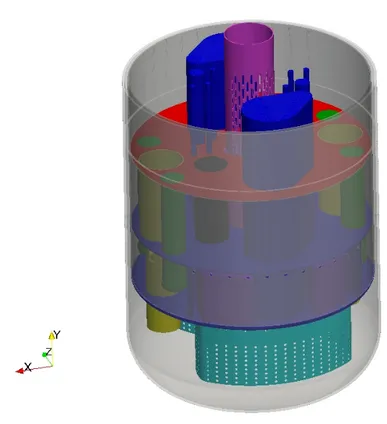
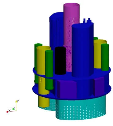
In this section, a descritpiton of each component of the geometry of the MYRRHA reactor is made. However, it is important to point out that it has been evolving throughout the years. The geometry considered for this work is the version 1.6, whilst in the comparative document [4] it is the version 1.4. It is also relevant to note that given the fact that some areas of the geometry are very dense, porous media (described in 3.6.1) was applied in these same areas. In figures 3.1 and 3.2, the full geometry of the reactor is presented whilte in figure 3.3, the inside components of the reactor are shown.

3.6.1 Porous Media

The porosity is defined as the ratio between the volume of the fluid and the total volume of the media, and it’s represented by γ. It characterizes each porous zone and is used in the prediction of heat transfer in the porous media.

Darcy’s law (1856) links pressure drop and velocity in fluid flow through porous media. However, as velocities increase, a difference between experimental data and results obtained for Darcy’s law appears. This way, Darcy-Forcheimmer was obtained to link this discrepancy to inertial effects. Forcheimmer (1901) suggested to add a term to Darcy’s law representing kinetic energy [13]. −∆p_L = 1 ω(µ−→u ) + β(ρ − → u2₎ _(3.1) where: • ∆p – pressure drop

(30)

Chapter 3 • MYRRHA Geometry

Figure 3.1: Full geometry of MYRRHA reactor

Figure 3.2: Side perspective

• L – reference length (m)

• ω - permeability coefficient (m2₎

• β - Forchheimer coefficient (m−1₎

(31)

Geometry _{Chapter 3 • MYRRHA}

Figure 3.3: Inside components of the reactor

• u - velocity (m/s)

An additional flow resistance which takes a form of a source of mass forces is considered and is added to the source term of momentum balance equation.

The resultant standard equation as a momentum sink when adding the pressure losses caused by friction has two terms: one described by Darcy’s law, corresponding to losses due to viscosity, and the second one described by Forchheimer’s law, taking into account losses due to viscosity and inertia. Therefore, according to OpenFOAM’s porous media model, also used in ANSYS-Fluent, [13] [14], this equation is as follows:

S =−(µdu +1₂ρβu2) (3.2)

Where:

• d - Darcy coefficient (m−2₎

The viscous losses are not considered, only the inertial resistance (second term of ?? and ??). Once the expected pressure drop is known, the inertial resistance coefficient can be calculated according to the estimated flow rate:

C2= △pporous Lref p 2− ˜u 2 (3.3) Where: • ũ – superficial velocity

The Darcy-Forcheimmer law was implemented to module the porous media in the HX, in certain layers of the core and in the ACS.

(32)

3.6.2 Pumps

The pumps drive the flow field within the reactor. These are two HX/Pump casing, each one containing two HX and one pump.

The previous studies performed showed that the effect of the swirl created by the blades can be disregarded, as it does not influence parameters of interest for this study, for example pressure drops. Modelling the flow through the rotor would require meshing around the blades and mod-elling their dynamic behaviour. Moreover, this study only concerns the nominal flow conditions of the primary coolant loop. Consequently, the presence of the rotor can be neglected in the CFD model.

Two approaches to represent the primary coolant are possible: either an open system or a closed system. On 3.4 the geometry of the pumps can be seen.

In the first approach, the rotor area (annular volume between red and green ring) is neglected in the CFD model and the nominal mass flow rate (most important parameter of MYRRHA) is imposed at the pump’s outlet (green surface) with a value of 9440 kg/s under nominal condi-tions, while velocity conditions are detailed. Then, pressure is imposed at the pump’s inlet (red surface). In order to impose a certain amount of swirl to the flow, a tangential velocity component can be specified at the outlet.

Figure 3.4: Pump inlet (red) and outlet (green) surfaces

Nevertheless, in transient simulations (for example pump failure), a closed-loop system is the simplest way of insuring that the flow between the pump’s inlet and outlet is continuous. In order to balance the chosen mass flow rate, the flow motion is later activated by a momentum source applied to the rotor area and fixed. The balance between the inlet and outlet is given by: ˙ m(ub− ua) = paSa− pbSb+ Fm+ G +V (3.4) With: • G – gravity term • V – viscous term 12

(33)

Geometry _{Chapter 3 • MYRRHA} • Fm– momentum source

Computing the momentum source is important to balance the pressure difference in the vol-ume. This pump head compensates the natural pressure drops (through extensions, contrac-tions, holes…) and the pressure losses due to the porous media. However, the source should then be adjusted to provide the right mass flow rate.

3.6.3 Butterfly

The objective of the butterfly, or baffle, is to avoid any fuel element (FA) to get out of reach of the in-vessel fuel handling machine (IVFHM). It is located in the lower plenum. It has holes in its structure, in order to mix the flow in the lower plenum (42 of 5 cm diameter in the upper part and 774 of 8 cm diameter in the lower part).

The butterfly was not modelled as porous media as it would increase the mesh size and the flow passing through the holes is perpendicular to the shell. Due to its shape it is difficult to define a local reference coordinate system, and therefore it is not possible to set a very high tangential inertial resistance coefficient.

Figure 3.5: Butterfly

3.6.4 Core

This component has been modelled as a porous media. It is composed by:

• The central core, which consists of 5 porous rings with a height of 1.78 m, from the centre: the inner FA, combination of IPS+SR+CR, the outer FA, the inner dummies and the outer dummies.

• The area directly below the core: grid with cones that hold the FA in place. This grid makes the connection with the CRS (core restraint system). This area is considered as non-porous due to the small flow blockage from both axial and radial directions.

(34)

Chapter 3 • MYRRHA Geometry • The combination of IPS, SR and CR can be approximated as a single ring since these com-ponents are arranged separately between the FA, and therefore this is a non-negligible assumption momentum and heat transfer wise.

In 3.6 a) we can see the layers of the core modelled with the porous media approach. In 3.6 b) all the layers of the core are shown, as well as in 3.6 c) but with opacity.

Figure 3.6: Core

Figure 3.7: Distribution of porosity in core layers

In 3.7 the layers are represented in different colours, according to its porosity. The outer ring (in black) is a solid component, therefore not considered in the porous domain. It is referred to as core jacket and is the structural interface between outer hexagonal fuel assemblies and the round core barrel. It maintains the core geometry and acts as radiation shielding, protecting the core barrel. As mentioned in 3.6.1, the Rehme correlation was used to calculate the expected 14

(35)

Geometry _{Chapter 3 • MYRRHA} pressure drop in the core.

It can be considered that an uniform pressure drop of 1.7 bar is expected in the core, despite the different porosity and mass flow rates in some of the central core rings. From the lower plenum up to the free surface (radial losses through the barrel holes included) the pressure drop is estimated to be around 2 bar.

The superficial velocity is calculated by multiplying the real velocity by the media’s porosity. In conclusion, each porous media is defined by the γ value and by the inertial resistant coefficient (C2,r,C2,y) in the radial and axial direction, respectively.

The value of C2,r is assumed to be high (1000 m−1) in the core region as the flow is blocked

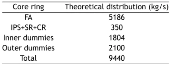
in the radial direction, given the presence of various instrumentation tubes and guiding vanes. The cross sections of the rings are determined according to the fractions of core positions take. When working in critical configuration, the core of MYRRHA consists of 69 fuel assemblies, 24 inner dummies, 42 outer dummies, 3 SR, 6 CR and 7 IPS. Then, it is possible to determine the mass flow rate distribution based on these cross sectional areas and a nominal total mass flow rate of 9440.4 kg/s. In the following table 3.1 the expected mass flow distribution is presented:

Table 3.1: Theoretical mass flow rate distribution in the core Core ring Theoretical distribution (kg/s)

FA 5186

IPS+SR+CR 350 Inner dummies 1804 Outer dummies 2100 Total 9440

In normal operation, the pressure drop is determined according to the pressure drop in the FA. By recurring to the Rehme correlation for a fuel bundle as a function of the local Reynolds number, f(Re), it is possible to estimate the value of the pressure drop:

△ P = fL_Dpin

eq

0.5ρu2 (3.5)

where:

• u – local flow velocity • Lpin– pin length

• Deq– equivalent diameter

• f – friction factor

The friction factor is given by: f = (64 ReF 0.5₊ 0.0816 Re0.133F 0.9335_)N rπ(Dr+ Dw) 1 St (3.6) With: • Nr- number of pins

• Dr– clad outside diameter

(36)

Chapter 3 • MYRRHA Geometry • F – geometrical factor

• St - Stanton number

The geometrical factor value is of 1.225. For the FA inner core, outer core and for the core inner dummies, the Re and f are calculated by recurring to the previous equations, implemented within the numerical model. The inner dummies are modelled as the FA rings since these have the same flow rate and pressure drop.

With respect to the IPS+SR+CR and core outer dummies, the axial resistance was kept constant and first approximated with base on the desired mass flow rate distribution, from which an average LBE velocity can be extracted, being the values adjusted to be more approximated to the distribution.

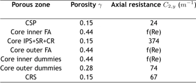
In the case of the core support plate (CSP) and the CRS regions, the axial resistance coefficient was calculated in order to reach a total pressure drop of 2 bars across the whole central region of the reactor. A summary of the final porous media parameters can be found in the following table 3.2

Table 3.2: Porous media parameters in the core

Porous zone Porosity γ Axial resistance C2,y(m−1)

CSP 0.15 24

Core inner FA 0.44 f(Re) Core IPS+SR+CR 0.15 374

Core outer FA 0.44 f(Re) Core inner dummies 0.44 f(Re) Core outer dummies 0.28 74

CRS 0.15 67

3.6.5 Core heat source distribution

The heat in the core is modelled as a volumetric heat source of 100 MW in total and is limited to the inner and outer FA rings, where the nuclear reaction is noteworth. The foreseen radial power distribution , which can be seen in 3.8, is approximated by a third order polynomial to approach an integrated power of 24.6 MW and 75.4 MW in the inner and outer FA rings.

Figure 3.8: Radial power distribution in the MYRRHA reactor core

(37)

Geometry _{Chapter 3 • MYRRHA} The final expression used to model the core heat source distribution is given in W /m3_by:

Qcore(r, y) = 1.86 cos ! π 1.78(y + 0.29) " (309.45r3_{− 637.4r}2+ 9.13r + 214.8) (3.7)

3.6.6 Barrel

Located in the centre of the reactor, the barrel is an integral part of the core support structrue, CSS. Its function is to guide the LBE flow from the lower (cold) plenum to the upper (hot) plenum through several holes which allow the hot LBE originating from the core flow into the upper plenum. The ACS (Above core structure) contains a number of guide tubes and instrumentation tubes and is surrounded by the upper part of the barrel.

Figure 3.9: Barrel

Two chinmeys that contain the actuating rods are located on the sides of the barrel, as seen in figure 3.10. Their purpose is to lower the CRS and are neglected from the CFD model as they are considered solid zones. The free surfaces are shown in green and the hot plenum in orange in 3.10.

The top and lower part of the ACS are modelled with the porous media approach, with a porosity of 1. The inertial resistance coefficient is set to 2 m−1 _{in the axial direction while the radial}

flow blockage is imposed to be C2,r = 1000 m−1 From the free level of LBE to just above the

outlet nozzles of the fuel assemblies, the ACS is also modelled as a porous media. Derivation of porous media properties of the ACS were based on the book [15].

3.6.7 Free surfaces

Regarding the free surfaces, some assumptions are made. The LBE free-surfaces are approached by a free slip condition and modelled as zero shear slip walls since their level is not expected to vary much, given the steady-state nature of the problem.

(38)

Figure 3.10: Hot plenum and barrel free surfaces

3.6.8 Primary Heat Exchanger

Once the heat is collected from the nuclear reaction, the pumps aspirate the existing hot LBE in the hot plenum into the four heat exchangers (HX). In the heat exchangers, the heat is transferred to the secondary coolant, consisting of a mixture of liquid and steam water like in most nuclear power plants. Consequently, the cooled LBE exits the HX’s and is sucked into the pumps and expelled at a higher pressure into the cold plenum.

Figure 3.11: Primary Heat Exchanger scheme

In 3.11 we can see the design of the FASTEF HX. The LBE flows outside the water tubes down-wards, while the two-phase water flows upwards. During normal operation, one of the HX’s main functional requirements is to remove the power generated by the reactor core and all of the other sources. Taking these requirements into account, it is designed to extract 110% of the 18

(39)

Geometry _{Chapter 3 • MYRRHA} nominal core power. In conclusion, the number and dimensions of the water tubes achieved to be enough for the HX to extract 27.5 MW is of 684 water tubes with an external diameter of 16 mm.

To avoid representing the numerous water tubes in the CFD model, the HX is simplified by using the porous media approach, which can be seen in green in figure 3.12 occupying all the volume of the HX. Its upper part is limited by the LBE free surface level.

Figure 3.12: Primary Heat Exchanger

Therefore, the only represented tube is the feed water pipe in the centre, subtracted from the numerical domain. The porosity is calculated with base on the cross-sectional area of the feed water pipe and the smaller water tubes. The pressure drop is obtained with the theoretical average velocity, and therefore the inertial resistance coefficient is calculated. The values for the porous media definition in the HX can be found in the following table 3.3:

Table 3.3: Porous media parameters in the HX

Porous zone Porosity γ Axial resistance C2,y(m−1) Radial resistance C2,x(m−1)

HX 0.62 1.55 0.32

The heat transfer between the primary and secondary coolant is represented in the CFD model by a variable heat sink positioned in the HX porous zone.

To obtain the Nusselt number (Nu), the following correlation derived by P.A Ushakov (1977) for the flow of a liquid metal in triangular or hexagonal rod bundles arrays [16] with a pitch-to-diameter ratio (P/D) between 1.3 and 2.0 and Peclet numbers between 1 and 4000 [17] and constant qw is applied: N u = 7.55 #_P D $ − 20 #_P D $−13 + 3.67 90(P /D)2P e( 0.19₍P D)+0.56) (3.8)

where P/D is the pitch-to-diameter ratio and Pe is the Peclet number given by:

(40)

Chapter 3 • MYRRHA Geometry with Re = ρ umagnDH µ P r = µCP λ (3.10) where:

• ρ - density of the fluid (kg/m3₎

• umagn- velocity magnitude

• DH - hydraulic diameter of the pipe (m), DH = 4A

P where A is the cross-sectional area and P is the wetted perimeter

• µ - dynamic viscosity of the fluid (Pa·s = N·s/m2_{= kg/(m·s))}

• Cp - specific heat (J kg−1K−1)

• λ - thermal conductivity (W/m.K)

In the simulation, the local velocity magnitude umagnis considered to calculate the local heat

transfer described by Nu. The latter is then used to determine the heat transfer coefficient he

on the LBE side, given by:

he=N uλ

DH

(3.11) Now we can finally obtain the total local heat transfer U, while considering the water tube’s heat transfer resistance R and the heat transfer coefficient hi on the waterside:

U =# ₁ 1 he

+ R + 1 hi

$ (3.12)

To obtain the volumetric heat sink SP HX in the core, the following equation is used:

SP HX =

U Aexchange(T− Twater)

VP HX· FP HX

(3.13) With:

• Aexchange- water tubes’ exchange surface

• VHX - HX’s Volume

• T − Twater - local temperature difference between the LBE and the water

• FHX - factor to adjust the heat that is removed

The water temperature is considered to be 473.15 K (200 ºC). FHXis fixed to 0.52 so that around

25.5 MW are removed by each HX when heat losses are neglected.

3.6.9 Diaphragm

The diaphragm’s function is to separate the cold low pressure LBE from the hot high pressure LBE, therefore it separates the cold and hot plenum. It is composed by three different volumes: central volume surrounding the core, the volume surrounding the IVFS and the volume of the pump boxes. It incorporates two horizontal plates connected by vertical shells and tubes and with seeveral volumes in between. Two of these volumes house the pumps and the PHX. The connecting tubes, called chimneys, are the penetrations for the components which have to 20

(41)

Primary coolant: Lead-Bismuth Eutectic _{Chapter 3 • MYRRHA} access the cold plenum. The low pressure cold LBE originating from the PHX is aspired by the primary pump into the pump boxes, therefore separating the stresses between the lower plate and the upper plate, induced by the pressure difference and thermal gradient. In figure 3.13 the diaphgram can be seen in red and the main walls in green.

Figure 3.13: Diaphgram

3.6.9.1 IVFS

Four racks, each capable of storing half a core, with 76 positions to place the Fuel Assemblies, compose the In Vessel Fuel Storage. In the CFD model, the different individual positions are represented with the porous media approach (as mentioned in 3.6.1, surrounding all the storing positions. The FA are inserted in the pipes of the IVFS and prevail until their residual heat has sufficiently decayed. It is assumed that all racks are fully occupied by the FA. Therefore, the same parameters are considered for both IVFS and FA rings porous media, as specified in section 3.6.1. The stored FA release some residual heat, making the IVFS an additional source of energy. Therefore, each FA has a uniform heat source in order to inject an extra 2MW in total. The loading and unloading of the assemblies to the IVFS is handled by two in-vessel fuel-handling machines, installed permanently in the reactor. Natural convection is also present, as the LBE is able to flow within the IVFS, contributing to cool down the FA. For this purpose, numerous holes are located in the cylindrical shell of the inner vessel, between the two plates of the IVFS casing. The IVFS was modelled with the Rehme Correlation and with a porosity of 0.44. The following figure 3.14 shows the porous media (IVFS) of the diaphgram in blue.

3.7 Primary coolant: Lead-Bismuth Eutectic

This section presents an overview of the primary coolant of the reactor.

(42)

Chapter 3 • MYRRHA Primary coolant: Lead-Bismuth Eutectic

Figure 3.14: IVFS

flux, high power density and short deployment of MYRRHA (start before 2020). Gaseous coolants were not an option because gases have a lower density in relation to liquids and therefore poor heat transfer characteristics, which is non-desirable for a fast reactor [18].

In a flexible irradiation facility like MYRRHA, fire safety risks have to be carefully taken into ac-count. Therefore, sodium was not elected as coolant due to its chemical reactivity with water and air. Given these restrictions, the alternative liquid metals are lead (Pb) and lead-bismuth eutectic (LBE), currently considered the potential candidates for the coolant of new genera-tion fast spectrum nuclear reactors and ADS and for liquid spallagenera-tion neutron sources (Sobolev, 2012). However, these coolants present the disadvantage of having a high corrosion rate of steels at high temperatures (>773 K). To avoid corrosion problems it is desirable that the pri-mary systems function at low temperatures. Since the LBE presents a low melting temperature (398 K) while lead has a higher melting temperature (600 K), it allows low operation tempera-ture range resulting in lower corrosion rates and in easier maintenance, and was therefore the chosen option.

Metals and the other media differ mainly because metals have a significantly higher thermal con-ductivity λ [W m−1_K−1_{] and lower specific heat capacity c}

p[J kg−1K−1]. For the same velocity,

LBE presents larger Re, because its kinematic viscosity ν [m2_s₋₁_{] is often smaller than that of}

air or water. Combining all these properties, we can obtain a characteristic dimensionless quan-tity, the Prandtl number Pr. Physically, the Prandtl number weights the transport coefficients of momentum (ν) and thermal energy (α) and is therefore a fundamental parameter to take into account in convective heat transfer problems. It is important to note that this parameter depends only on the physical properties of the fluid, being independent of the velocity or the geometry. It is defined as the ratio of momentum diffusivity to thermal diffusivity in a fluid:

P r = cpµ λ = ν α where α = λ ρcp (3.14)

The LBE presents a low Prandtl number, meaning that the thermal diffusivity dominates and that its material properties are highly dependant on temperature Liquid metals present Prandtl 22

(43)

Primary coolant: Lead-Bismuth Eutectic _{Chapter 3 • MYRRHA} numbers in a lower range: 0.002 ≤ Pr ≤ 0.06.

Nevertheless, LBE has some disadvantages. Due to the existence of bismuth, radioactive capture of neutrons occurs, leading to the production of the alpha-active polonium. Still, it is the best option between the liquid metals, since the other alloys of lead without bismuth require very low oxygen content in coolant and their properties are not yet very well known [12].

3.7.1 Properties

Linear or second order interpolation of experimental data collected in the database for liquid LBE returns for the LBE density ρLBE, conductivity λLBEand heat capacity CPLBE:

ρLBE= 11096− 1.3236 T (3.15)

λLBE= 3.61 + 1.517× 10−2T− 1.741 × 10−6 T2 (3.16)

CPLBE= 159− 2.72 × 10−2T + 7.12× 10−6 T

2 _(3.17)

As for dynamic viscosity µLBE, the viscosity database yields the following correlation:

µLBE= 4.94× 10−4e754.1/T (3.18)

These equations were implemented within myrrhaSimpleFoam in the file related to the proper-ties of the LBE. In the isothermal scenario, the density and the dynamic viscosity are fixed to ρLBE= 10377.1 kg/m3 and µLBE= 0.00198P a.s.

(44)

(45)

Chapter 4

Numerical set up

In this chapter, the numerical characteristics and set up of the simulation are exposed. The present work considers a steady-case of an incompressible turbulent flow.

A flow with constant velocity, pressure, density, etc., at any position and that does not change with time, is a steady flow [19].

A turbulent flow is characterized by chaotic changes in pressure and flow velocity. Amongst others, it has the following characteristics:

• Irregularity: therefore turbulent flows are analysed statistically

• Diffusivity: the enhanced mixing and increased rates of mass, momentum and energy transports that characterizes turbulent flows.

• Near walls, since they are solids, the flow has a distinct structure called boundary layer. Here, the velocity of the fluid decreases to zero, so we can see the “no-slip” condition, i.e, the fluid velocity is the same as the boundary velocity and therefore has no relative slip. This is due to viscosity, ν, which is a fluid’s resistance to flowing or fluid friction. The higher the viscosity, the more the fluid resists to flowing.

4.1 Reynolds Decomposition

The Reynolds decomposition decomposes the flow property ϕ in a steady mean component φ and a time varying fluctuating component ϕ′_{(t) with zero mean value, so we obtain:}

ϕ(t) = φ + ϕ′(t) (4.1)

Turbulent eddies originate fluctuations in velocity. In turbulent flow, the velocity record is de-composed in both a mean and a turbulent component, i.e, instantaneous quantity is dede-composed into its time-averaged and fluctuating quantities [20].

u(t) = u + u′(t) v(t) = v + v′(t) (4.2) Where u is the longitudinal velocity and v is the vertical velocity, both varying in time due to turbulent fluctuations.

Due to the random nature of eddies, a statistical approach to the turbulent motions can be done. Theoretically, the velocity record is continuous and the mean can be evaluated through integration. Nonetheless, in practice the measured velocity records are a series of discrete points, ui. The mean velocity

u = % t+T t u(t)dt = 1 N N & 1 ui (4.3)

(46)

Chapter 4 • Numerical set up Numerical methods where, time T is much longer than any turbulence time scale, but much shorter than the time-scale for mean flow unsteadiness. The turbulent fluctuations are given by:

• Continuous record: u′_{(t) = u(t)}_{− u}

• Discrete points: u′

i= ui− u

The turbulence strength, which is considered to be the standard deviation urms of the set of

random velocity fluctuations u′

i, is given by: urms= ' u′_(t)2₌ ( ) ) * 1 N N & i=1 u′ i 2 _(4.4)

where the subscript rms stands for root-mean-square.

The higher urms, the higher the level of turbulence. Another consideration to take into account

is that shear produces turbulence, and, the stronger the shear, the stronger the turbulence.

4.2 Numerical methods

Turbulence originates eddies with a wide range of length and time scales, interacting in a dy-namically complex way. Therefore, it is important to capture the effects of turbulence in the flow. For that purpose, three categories of numerical methods exist:

• Turbulence models for Reynolds-averaged Navier-Stokes (RANS) equations • Large eddie simulation (LES)

• Direct numerical simulation (DNS)

For this study case, the RANS approach is used, as it requires modest computing resources for reasonably accurate flow computations. An overview of this method is made in the following sub-section 4.2.1.

4.2.1 Reynolds-averaged Navier-Stokes equations

The following instantaneous continuity equation and Cartesian co-ordinate system of equations governs every turbulent flow for the velocity vector u. The vector has the component-x u, component-y v and component-z w:

div u = 0 (4.5) ∂u ∂t + div(u u) =− 1 ρ ∂p ∂x+ ν div (grad(u)) (4.6) ∂v ∂t + div(v u) =− 1 ρ ∂p

∂y + ν div (grad(v)) (4.7)

∂w ∂t + div(w u) =− 1 ρ ∂p ∂z+ ν div (grad(w)) (4.8)

With the effects of fluctuations on the mean flow, using the Reynolds decomposition in the pre-vious equations and replacing the flow variables u and p by the sum of a mean and a fluctuating component, we obtain:

u = U + u’ u = U + u′ _{v = V + v}′ _{w = W + w}′ _{p = P + p}′ _(4.9)

(47)

Numerical methods _{Chapter 4 • Numerical set up} Considering the continuity equation and taking the time average, first:

div u = div U (4.10)

And thus we have the continuity equation for the mean flow, where U is the velocity steady mean value:

div U = 0 (4.11)

The Navier-Stokes equations are time averaged before a numerical method is applied. Rewriting the time averages of the individual terms in the x-momentum equation we obtain:

∂u ∂t =

∂U

∂t div(uu) = div(UU) + div(u′u’) (4.12)

−1_ρ∂p_∂x =₋1 ρ

∂P

∂x ν div(grad(u)) = ν div(grad(U )) (4.13) Substitution of these terms gives the time-average x-momentum equation:

∂U

∂t + div(U U) + div(u′u’) = − 1

ρ+ ν div(grad(U )) (4.14) The same applies for the y- and z-momentum equations. We can verify that due to the process of time averaging, a new term that was not in the instantaneous equations appears: div(u′_{u’). This}

term consists of products of fluctuating velocities and are associated with convective momentum transfer due to turbulent eddies [5].

In conclusion, we obtain the Reynolds-averaged Navier-Stokes equations, where the new terms are placed on the right hand side of the equations to highlight their role as additional turbulent stresses on the mean velocity components U, V and W:

∂U ∂t + div(U U) =− 1 ρ ∂P ∂x + ν div(grad(U )) + 1 ρ +_∂( −ρu′2 ∂x + ∂(_−ρu′_v′ ∂y + ∂(_−ρu′_w′ ∂z , (4.15) ∂V ∂t + div(V U) =− 1 ρ ∂P ∂y + ν div(grad(V )) + 1 ρ +_∂( −ρu′_v′ ∂x + ∂(−ρv′2 ∂y + ∂(−ρv′_w′ ∂z , (4.16) ∂W ∂t + div(W U) =− 1 ρ ∂P ∂z + ν div(grad(W )) + 1 ρ +_∂( −ρu′_w′ ∂x + ∂(−ρv′_w′ ∂y + ∂(−ρw′2 ∂z , (4.17) These equations represent the transport equations for the mean flow variables and the effects of turbulence on mean flow properties, reducing the computational effort. Since the mean flow is steady, time derivatives disappear. To model the extra terms that appear due to the interaction between turbulence fluctuations, classical turbulence models are used (like the κ − ε model and the Reynolds stress model), as these allow predicting the Reynolds stresses and the scalar transport terms and close the system of mean flow equations.

4.2.2 RANS Temperature Equation

To model turbulent flows, nowadays, the most used methods are based on the time-averaged Navier-Stokes equations (RANS), referred to as the Reynolds equations (referrenced in chapter 4 and section 4.2.1).The main specific features of liquid metals are related to the turbulent transport of heat. Regarding the transport of momentum, their behaviour is similar to other Newtonian fluids [12]. However, the transport of momentum has a strong influence in the energy

(48)

Chapter 4 • Numerical set up Standard κ − ε model balance. Therefore, modelling turbulent heat flux is always coupled to a model for the turbulent transport of momentum. For all theoretical considerations regarding turbulent heat transfer, a central problem is given by the evaluation of the turbulent heat flux u′

iT′. Consequently, it is

frequently modelled using the concept of the thermal eddy diffusivity (αt) and the corresponding

turbulent Prandtl number (P rt), which we will see with more detail on the following section.

Regarding liquid metal flows, for a steady steate incompressible flow and assuming that the molecular heat flux is governed by the Fourier law of conduction and that there are no source or sinks of mass, momentum and energy, the following energy time-averaged transport equation considering the Reynolds decomposition is obtained [12]:

ui ∂T ∂xi = ∂ ∂xi - ν P r ∂T ∂xi − u ′ iT′ . _(4.18) and considering:

• Thermal diffusivity for a fluid: α = ν P r • For turbulent components: αt= νt

P rt & j ∂(UjT ) ∂Xj =& j ∂ ∂Xj -α ∂T ∂Xj − u ′ JT′ . + Q (4.19)

We can verify that a new term appears in the energy equation due to time averaging, the turbulent heat flux:

qi′′= u′iT′ (4.20)

Where αef f is the effective thermal diffusivity.

The following equation for the temperature is implemented:

▽ ·(−→U T ) =_{▽ · (α}ef f ▽ T ) + Q (4.21)

Likewise modelling the extra terms that appear in the Navier-Stokes equations due to time averaging, the turbulent heat flow needs to be modelled as well for the closure of the problem. For this purpose, the Reynolds Analogy is used.

4.3 Standard

κ

− ε

model

This model is a general description of turbulence that allows for the effects of transport of turbulence properties by convection and diffusion and for production and destruction of turbu-lence. RANS turbulence models are classified according to the number of additional transport equations that need to be solved along with the RANS flow equations, and in the case of this model, two transport equations (PDEs) are solved: one for the turbulent kinetic energy κ and a further one for the rate of dissipation of turbulent kinetic energy ε. It is assumed that the turbulent viscosity µ is isotropic. There is also a kinematic turbulent or viscosity ν given by: νt= µt/ρ in m2/s. The mechanisms that affect the turbulent kinetic energy are the main focus

in this model. Eddy viscosity or (turbulent viscosity) is given as follows in Pa.s: µt= ρCµ

κ2

ε (4.22)

Numerical simulation of the MYRRHA reactor design v1.6

UNIVERSIDADE DA BEIRA INTERIOR

Engenharia