A FLEXIBLE DECISION SUPPORT TOOL FOR MAINTENANCE FLOAT SYSTEMS - A
SIMULATION APPROACH
Francisco Peito(a), Guilherme Pereira(b), Armando Leitão(c), Luís Dias(d), José A. Oliveira(e)
(a)
Industrial Management Dpt., Polytechnic Institute of Bragança (b)
Research Centre ALGORITMI, University of Minho (c)
Industrial Engineering and Management Dpt., Faculty of Engineering, University of Porto (d)
Research Centre ALGORITMI, University of Minho (e)
Research Centre ALGORITMI, University of Minho
(a)
[email protected], (b)[email protected], (c)[email protected], (d)[email protected], (e)[email protected]
ABSTRACT
This paper is concerned with the use of simulation as a decision support tool in maintenance systems, specifically in MFS (Maintenance Float Systems). For this purpose and due to its high complexity, in this paper the authors explore and present a way to develop a flexible MFS model, for any number of machines in the workstation, spare machines and maintenance crews, using Arena simulation language. Also in this paper, some of the most common performance measures are identified, calculated and analysed. Nevertheless this paper would concentrate on the two most important performance measures in maintenance systems: system availability and maintenance total cost. As far as these two indicators are concerned, it was then quite clear that they assumed different behaviour patterns, especially when using extreme values for periodic overhauls rates. In this respect, system availability proved to be a more sensitive parameter.
Keywords: Simulation, Discrete Event Simulation, Maintenance, Preventive Maintenance, Waiting Queue Theory, Float Systems.
1. INTRODUCTION
According to (Pegden et al., 1990), simulation can be understood as the process of construction of a real system representative model, as well as an experimental process aiming to a better understanding of their behavior and to assess the impact of alternative operations strategies. Thus, simulation may also be considered as a decision support tool that allows to predict and to analyze the performance of complex systems and processes as they are in many real systems. In addition, with the use of simulation we acquired a capacity to forecast and to achieve quickly the importance of taking some decisions about the system under analysis.
In some real systems like production areas, services such as transport companies, health service systems and factories, the main goal is to achieve high levels of competitiveness and operational availability. In this environment the need for equipment to work continuously is essential in order to maintain high levels of productivity. This is why MFS has an important role
on equipment breakdown and production stoppage has a high and direct impact on production process efficiency and, as a consequence, on their operational results. Therefore, maintenance control and equipment use optimization become not only an important aspect for the mentioned reasons, but also for personnel security matters and to prevent negative environmental impact. This maintenance control and optimization of equipment utilization can be achieved implementing preventive maintenance actions that increase equipment control and avoid unexpected stoppage. However, to overestimate these actions makes the maintenance costs too high for the required availability.
The integration of the maintenance management with materials and human resources is an advantage in production systems that involve identical equipment such as float systems – involving the existence of spare equipment to replace those that fail or need review. Then, the direct and indirect costs due equipment stoppage are minimized and the level of production or service requirements fulfilled. Although the existence of spare equipment is important to maintain the production process working it is recommended to keep the number of spare equipment in an optimal level for economic reasons.
Mainly due to the non-existence of a specific simulator for the maintenance field, we had a great difficulty in choosing an appropriate simulation tool. However, (Dias et al., 2005) had a definite contribution as far as the simulation tool decision is concerned.
In fact, the choice of Arena® as a simulation language was based on the fact that its hierarchical structure offers different levels of flexibility, thus allowing the construction of extremely complex models, allied to a strong visual component (Kelton et al., 2004; Dias et al., 2011; Dias et al., 2006; Pidd, 1993 and Pidd, 1989).
Having referred the importance of studying MFS, the research background section of this paper will focus on the literature review on analytical models, but also on some type of simulation metamodels for this type of maintenance systems.
of analysing system availability and total maintenance cost, as global efficiency measures.
The following section describes new developments on a previous simulation model towards flexibility. In fact, the model presented in (Peito et al., 2011) will gain the capacity to automatically generate a specific simulation program for each specific MFS desired. The program will then be adapted for specific situations with no need of further coding effort. In fact the new proposed tool is intended exclusively to give a response to a type-standard configuration of MFS. Nevertheless, within this type-standard configuration, the user could easily evaluate different strategies under different number of resources available (active machines, maintenance crews and spare machines). This way, the resulting MFS model aims to fill a gap in terms of computer solutions currently existing for this specific type of maintenance systems.
Then we present some results of both global efficiency measures under consideration, in order to evaluate its sensitivity, its precision and its robustness.
Conclusions and Future Developments are the closing sections for this paper.
2. RESEARCH BACKGROUND
A literature survey on the field of maintenance systems, regarding the use of discrete event simulation, shows a significant number of scientific publications. Recently, (Alabdulkarim et al., 2013) present a complete set of research works where maintenance costs, maintenance reliability, maintenance operations performance, are some of the most important issues discussed. (Chen and Tseng, 2003), however, are the only authors which main focus is MFS.
In this respect (MFS), (Lopes 2007) refers some studies where simulation has been used to produce results based on specified parameters. Due to the fact that these simulation models were only concerned with the input/output process, without dealing with what is happening during the simulation data process, some metamodels have emerged (Madu and Kuei, 1992b; Madu and Lyeu, 1994; Kuei and Madu, 1994; Madu, 1999; Alam et al., 2003). The metamodels express the input/output relationship through a regression equation. These metamodels can also be based on taguchi methods (Kuei and Madu, 1994) or on neuro networks (Chen and Tseng, 2003). These maintenance system models were also recently treated on an analytical basis by (Gupta and Rao, 1996; Gupta, 1997; Zeng and Zhang, 1997; Shankar and Sahani, 2003; Lopes, 2007). However, the model proposed by (Lopes, 2007) is the only one that deals, simultaneously, with three variables: number of maintenance teams, number of spare equipment, and time between overhauls, aiming the optimization of the system performance. Although this proposed model already involves a certain amount of complexity it may become even more complex by adding new variables and factors such as: a) time spent on spare equipment transportation, b) time spent on spare equipment installation; c) the introduction of more
or different ways of estimating efficient measures; d) allowing the system to work discontinuously; e) speed or efficiency of the repair and revision actions; f) taking into account restrictions on workers timetable to perform the repair and revision actions; g) taking into account the workers scheduling to perform the repair and revision actions; h) taking into account the possibility of spare equipment failure; etc. Anyway these mentioned approaches would aim at ending up with MFS models very close to real system configurations. In fact, the literature review showed that most of the works published, involving either analytical or simulation models, concentrate on a single maintenance crew, or on a single machine on the workstation or even considering an unlimited maintenance capacity – thus overcoming the real system complexity and therefore not quite responding to the real problem as it exists.
As far as the model presented by (Lopes et al., 2005; Lopes et al., 2006; Lopes, 2007) is concerned it is assumed that systems works continuously, its availability is not calculated and the system optimization is only based on the total maintenance cost per time unit. Moreover, it considers that the total system maintenance cost is the same without taking into account the number of machines unavailable, which in many real situations it is not the best option. Finally the referred analytical model only allows that its failures occur under an homogeneous Poisson process (HPP).
Another important aspect on the companies’ management strategic definition is to have their tasks correctly planned. To help this planning procedure it is important to know different indicators such as: machine availability, equipment performance and maintenance costs, among others. Therefore one should consider new factors that affect these float systems indicators, such as the possibility of some machine failure, efficiency, repair time, etc.
Moreover, when preventive maintenance policy is used, the time for individual replacement is smaller than time for group replacement. It means that the latter situation requires more machine on the process to be stopped, and also implies an increase for a certain time, on the maintenance crews.
3. DESCRIPTION OF THE MFS
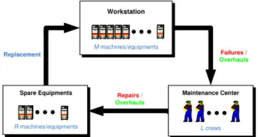
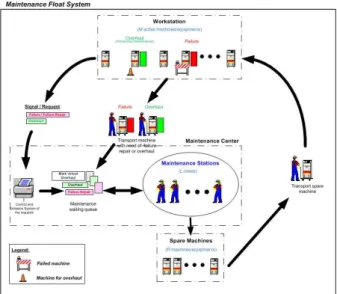
Our model represents a typical Maintenance Float System (MFS) and it is composed of a workstation, a maintenance center with a set of maintenance crews to perform overhauls and repair actions and a set of spare machines (Figure 1). The workstation consists of a set of identical machines and the repair center of a limited number of maintenance crews and a limited number of spare machines. However, the model we have adopted, being a typical MFS, presents certain specificities both as far as the philosophy of the maintenance waiting queues are concerned, and related to the management of the maintenance crews.
Workstation
Spare Equipments Maintenance Center
Failures / Overhauls
Repairs /
Overhauls
Replacement
M machines/equipments
L crews
R machines/equipments
Figure 1: Typical Maintenance Float System
This model follows the one proposed and developed by (Lopes, 2005; Lopes et al., 2006; Lopes et al., 2007), considering M active machines, R independent and identical spare machines and L maintenance crews The active machines considered operate continuously. Machines that fail are taken from the workstation and sent to the maintenance park waiting queue, where they will be assisted according to arrival time. Machines that reach their optimal overhaul time are kept in service until the end of a period T without failures. However they will be also kept on a virtual queue to overhaul. If the number of failed machines plus the number of machines requiring overhaul is lower than the number of maintenance crews available, machines are replaced and repaired according to FIFO (First In First Out) rule. Otherwise if it exceeds the number of maintenance crews, the machines will either be replaced (while there are spare machines available) or will be sent to the maintenance queue. The machines that complete a duration period T or time between overhauls in operation without failures are maintained active in the workstation, where they wait to be assisted, and they are replaced when they are removed from the workstation, to be submitted to a preventive action. Its replacement is assured by the machine that leaves the maintenance center in the immediately previous instant. If an active machine happens to fail it waits for the accomplishment of an overhaul, then it will be immediately replaced, if a spare machine is available or as soon it is available.
In this version of our model it is assumed that the M active machines of the workstation have a constant failure rate while the model runs.
Time between failures are assumed as independent and identically distributed following an Exponential Distribution for all machines (failures occur under a
Homogeneous Poisson Process). However, during a simulation run, this value could be adjusted based on time between overhauls. Obviously a smaller time between overhauls implies greater time between failures.
As far as time to overhaul and time to repair are concerned, we have assumed the Erlang-2 distribution, even though considering overhaul time significantly lower than the repair time.
Now, for our MFS, the variables used are the following:
1.
Number of active machines (M);2.
Number of maintenance crews (L); 3. Number of spare machines (R); 4. Machine- Overhauls rate (λrev); 5. Machine-Initial Failures rate (λf); 6. Crews-Repair rate (µrep); 7. Crews-Overhaul rate (µrev); 8. Failure cost (Cf);9. Repair cost (Crep); 10. Overhaul cost (Crev); 11. Replacement cost (Cs);
12. Cost due to loss production (Clp); 13. Holding cost per time unit (h); 14. Labour cost per time unit (k);
15. Time to convey and install spare machine (TConvInst).
The developed simulation model for our MFS allows us to estimate the following global efficiency measures:
a) Average system availability (AvgSAv);
b) Total maintenance cost per time unit (AvgTCu);
However, some other performance measures are also estimated, such as:
c) Average number of missing machines at the workstation (AvgMeq),
d) Average number of machines in the maintenance waiting queue (AvgLq);
e) Average waiting time in the maintenance waiting queue (Avg Wt);
f) Average operating cycle time (AvgD);
g) Probability of existing 1 or more idle Machines (Probim);
h) Probability of the system being fully active (Probs);
and still, some individual efficiency measures per machine or maintenance crew, i.e.,
i) Utilization rate per machine;
j) Utilization rate per maintenance crew;
k) Number of overhauls and repair actions performed per maintenance crew;
4. INCREASING FLEXIBILITY OF THE SIMULATION MODEL
The Arena® simulation language environment, used in the previous development (see details on Peito et al., 2011), has been now revisited, aiming to give flexibility to the previous model. The user, now, would be able to automatically generate a simulation program according to specific characteristics of the MFS, namely varying the number of active machines (M), the number of maintenance crews (L) and the number of spare machines (R). However, the steps towards the development of the previous simulation model were all kept and are presented in Figure 2, for a better understanding of the simulation model developed.
Figure 2: Steps for simulation model development
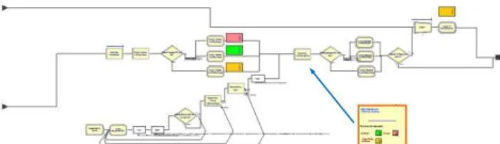
Figures 3 and 4 explicit the global logical simulation model before and after gaining flexibility, underlining its different developed components:
1. Active machines (workstation); 2. Statistics 1 (Recording Machines Tup); 3. Maintenance queue;
4. Machines’ transportation (by the maintenance crews);
5. Spare machine request;
6. Maintenance center (set of maintenance Stations);
7. Release machines to the set of spare machines; 8. Statistics 2 (Recording Machines Tup and
Tdown);
9. Spare machines (in the start of the system).
This logical model configuration choice was kept identical for the MFS (figures 3 and 4), providing again a clear global visualization of the undergoing operations and a great simplicity to make changes in the model. In fact the logical model, after increasing flexibility, will appear even more simplified – see Figure 4. The implementation of Arena resource sets, the inclusion of
indexed variables and data arrays and also a set of control variables, replacing previous Arena internal variables, have definitely contributed to a simplified model.
Figure 3: Arena® Logic Model before increasing flexibility
Figure 4: Arena® Logic Model after increasing flexibility
Figure 5: Generation and control system for repair and overhaul requests before increasing flexibility
A
A
B C
Figure 6: Generation and control system for repair and overhaul requests after increasing flexibility
necessary to guarantee absolute independence of each type of request for every machine. For this purpose, a mechanism for attribute identification was developed. With this mechanism, it is now possible to identify the state of each machine and the occurrence of every type of machine request (failure or overhaul), at any instant – entity number and color (see Figure 6, zone A).
In Figure 6 (Zone B), a small change has occurred. In fact, some Arena Blocks have been replaced by Arena Modules. This way, planned changes to some parameters are now easy to implement once Arena shows data in a simple table format.
Finally, Figure 6, Zone C shows four ReadWrite Arena modules, allowing the registration, in an excel worksheet, of the failure instants and the number of failures for each machine.
The maintenance waiting queue is defined through a synchronization of events between the component 3 and 4. In the component 4 (figures 7 and 8) there is a "control mechanism", which only allows a request to proceed if there is a free maintenance crew. Component 4 will now include the use of an Arena Resource Set for the maintenance crews, selecting the available maintenance crew that has the least number of services allocated.
The rules for the maintenance queue management were all kept unchanged. In fact, FIFO (First In First Out) is the rule for the maintenance queue management, except for the case when the total number of maintenance requests (overhauls plus repair actions) exceed the number of maintenance crews available – in this case, machines requiring repair action have priority over machines requiring overhauls.
Figure 7: Maintenance waiting queue before increasing flexibility
Maintenance Waiting Queue Nº Machines in
Ouverhauls Fails Overhauls Virtual-Marks Maintenance Waiting Queue
0
0 0 0
D
Figure 8: Maintenance waiting queue after increasing flexibility
Component 4 (figures 7 and 8) has also been changed and now includes an Assign Module in Zone D. Besides the identification of the maintenance crew and the machine transport state (for a spare machine or a failed machine or even a machine needing overhaul),
this Module also updates the number of maintenance crews that are free.
Figure 9: Request and activation of spare machines before increasing flexibility
E
Figure 10: Request and activation of spare machines after increasing flexibility
In component 5 (figures 9 and 10) that performs the request of a spare machine, performed by a maintenance crew, there is only a small change in Zone E, that is related with the demand with one free available machine. Now the model includes a Search Block that searches for a free machine.
In component 6 (Figure 11), the change is in the structure of the component. In fact, the discrete variables are now indexed discrete variables – this way, it is possible to individually save a set of performance indicators for both types of maintenance operations.
Figure 11: Identification and statistics of the states of the maintenance crew
Statistics 1
Statistics 2
Figure 12: Record statistics
Components 2 and 8 (Figure 12) which are responsible to record fundamental statistical data to calculate adequate efficiency measures, do not suffered any change.
Figure 13: Screenshot of the data input area before increasing flexibility
F
Figure 14: Screenshot of the data input area after increasing flexibility
This work, making previous simulation model gaining flexibility, allows the user to get a simulation model for any Maintenance Float System desired – regardless the number of active machines, the number of maintenance crews and the numbers of spare machines. After inputting these three values (Zone F, figures 14), the user will instantly get the appropriate simulation model automatically generated.
Figure 15: Screenshot of the detailed animation area of the Workstation (limited to M = 40, L = 18)
Figure 16: Screenshot of the global animation area of the Workstation
Figure 17: Screenshot of the Operating variables, Statistics and Graphics control area
The presentation of model animation (Figures 15 and 16) and output statistics (Figure 17) had changes relatively to the version presented in (Peito et al., 2011).
5. SIMULATION RESULTS AND DISCUSSION
This paper focus on the two general performance measures mentioned above – system availability and total maintenance cost per time unit, which were determined considering a Maintenance Float System with 10 active and identical machines (M), 5 spare machines (R) and 5 maintenance crews (L).
Simulation length was set to 9.000 hours (approximately one year) – warm-up period was set to 3.500 hours.
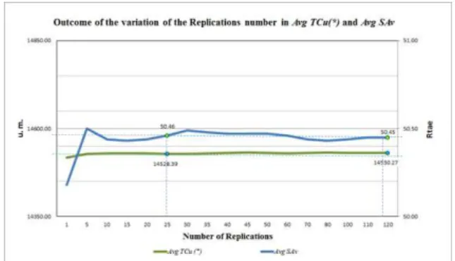
Figure 18: Outcome of the variation of the Replications number in AvgTCu and AvgSAv variables
replications – for an adequate system stabilization and results robustness for both performance measures (Figures 18 and 19) and also due to computational time required to run the model.
Figure 19: Outcome of the variation of the Replications number in AvgTCu(*) and AvgSAv variables
Bearing in mind the fifteen variables of MFS previously referred, simulation models were used to test and estimate the behavior of the two global efficiency measures mentioned on the previous section. Simulation models were carried out for (1-60) hypothetical scenarios with different overhauls rates (rev). These different overhauls rates are associated with different times between overhauls (T) which are defined accordingly to the preventive maintenance policy aiming the best option.
Table 1: Global efficiency measures outcomes in the MFS model after 25 replications
(Values estimated by simulation after 25 replication)
S c e n a r i o λrev (/hour) T (hour) AvgSAv (%) AvgTCu (m.u./hour) AvgTCu(*) (m.u./hour)
1 0,10 10,000 29,25 21064,60 17304,37
2 0,20 5,000 34,75 21127,96 16646,80
3 0,30 3,333 40,79 21065,24 15870,35
4 0,40 2,500 45,26 20915,39 15287,79
5 0,50 2,000 48,12 20751,46 14908,68
. . . . . . . . . . . . . . . . . .
52 9,00 0,111 48,71 20195,00 14776,87
53 15,00 0,067 48,52 20212,24 14807,21
54 20,00 0,050 48,54 20228,63 14815,57
55 25,00 0,040 48,56 20223,63 14814,18
56 30,00 0,033 48,54 20230,24 14816,98
57 35,00 0,029 48,62 20226,82 14811,16
58 40,00 0,025 48,54 20229,16 14820,31
59 45,00 0,022 48,50 20228,80 14822,78
60 50,00 0,020 48,52 20226,42 14815,55
(*)Considers that the cost of lost production changes in function of the number of active machines lacking in the system.
A first global analysis of the values presented in tables 1 and 2 indicate that the precision obtained on the three efficient measures analysed is different. An individual analysis of each measure indicates that AvgTCtu shows the smaller variation (MPO lower). In Table 1 it can also be observed that when T takes very small values (T≤0.111 or λrev≥ 9) the three efficient
measures [AvgTCtu, AvgTCTu(*) and AvgSAv] are kept practically unchangeable. This fact can be confirmed in Figure 20 or in Table 2 where the MPO for these values of T is extremely low, almost zero. On the other hand, when T assumes very high values (T≥2,5 or λrev≤ 0,4) the efficiency measures AvgTCTu(*) and AvgSAv present high MPO values in opposition to AvgTCtu that shows very small values. In Table 2 it can also be observed that AvgTCtu presents the lowest MPO average value of the three efficiency measures and that AvgSAv has the highest value.
Table 2: Observe percentage change in the global efficiency measures after 25 replications
MPO - Percentage change observed
S c e n a r i o AvgSAv AvgTCu AvgTCu(*)
1-2 15,83% 0,30% -3,95%
2-3 14,80% -0,30% -4,89%
3-4 9,87% -0,72% -3,81%
4-5 5,95% -0,79% -2,54%
. . . . . . . . . . . . 52-53 -0,14% 0,06% 0,10%
. . . . . . . . . . . . 58-59 -0,07% 0,00% 0,02%
59-60 0,04% -0,01% -0,05%
Max. 15,83% -0,79% -4,89%
Mean 0,80% -0,07% -0,27%
In order to simplify the interpretation and analysis of these global efficiency measures, figures 20, 21 and 22 pinpoint the maximum and minimum values (table 2 and 3) as well as other points considered relevant for the analysis.
Table 3: Maximum values of the main efficiency measures
Statistics
(Maximum) (/hour) λrev T (hour)
AvgSAv
(%) 50,70% 0,90 1,111
AvgTCu
(m.u./hour) 21127,96 0,20 5,000
AvgTCu (*)
(m.u./hour) 17304,37 0,10 10,000
Note: Red points in the graphics
Table 4: Minimum values of the main efficiency measures
Statistics
(Minimum) (/hour) λrev T (hour)
AvgSAv
(%) 29,25% 0,10 10,000
AvgTCu
(m.u./hour) 20096,90 1,80 0,556
AvgTCu (*)
(m.u./hour) 14518,77 1,20 0,833
Tables 3 and 4 show that the T value corresponding to the minimum value of AvgSAv corresponds the maximum value, as expected, of AvgTCu(*). When compared with the minimum of AvgTCu, there is a significant T gap ( 5 hours), although, its remains practically the same when the value of T changes from 5 to 10 hours (Figure 20).
When comparing the T value corresponding to the maximum value of AvgSAv with the T value corresponding to the minimum value of AvgTCu(*), there is only a small gap, which is clearly higher in the case of the T value corresponding to the minimum of the AvgTCu (Figure 22).
Table 5: Correlation coefficients
T AvgSav AvgTcu AvgTcu(*)
T 1 -0,9021 0,8279 0,9017
AvgSav -0,9021 1 -0,7980 -0,9986
AvgTcu 0,8279 -0,7980 1 0,8237
AvgTcu (*) 0,9017 -0,9986 0,8237 1
A careful analysis of the correlation coefficients of three efficiency measures, table 5, shows that T variations are better explained by AvgSav and AvgTCu(*) (90%). It is also verified that there is a high inverse correlation between AvgSav and AvgTCu(*) (99,8%). However when AvgTCu is compared with AvgTCu(*) or with AvgSav, the correlation coefficient decreases to 82,37% and to 79,80%, respectively. This partially explains why in tables 3 and 4 the T value corresponding to the maximum of AvgSav does not correspond exactly to the T value corresponding to the minimum of the AvgTCu and AvgTCu(*) and that difference being higher in the case of AvgTCu(*) (Figure 22).
Figure 20: Evolution of the AvgTCtu, AvgTCTu(*) and AvgSAv / Overhaul rate (λrev)
As it can be observed in Figure 20 and more clearly in figures 21 and 22, for the MFS analyzed, the three global measures of efficiency being studied only present small variations for values of rev between 0,10 and 9,00 (or T between 10,000 and 0,111 hours). For values of rev higher than 9.00 the three global measures of efficiency remain practically unchanged.
Figure 21: Evolution of the AvgTCtu, AvgTCTu(*) and AvgSAv / Overhaul rate (λrev)[Zoom Figure 20]
Figure 22: Evolution of the AvgTCtu, AvgTCTu(*) and AvgSAv/ Time between overhauls (T)
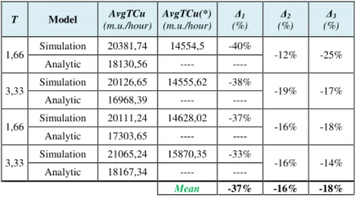
Table 6: Comparison among the AvgTCu values estimates by the simulation model and analytic model (Lopes, 2007)
T Model AvgTCu
(m.u./hour)
AvgTCu(*) (m.u./hour)
Δ1
(%) Δ2
(%) Δ3
(%)
1,66 Simulation 20381,74 14554,5 -40% -12% -25% Analytic 18130,56 ---- ----
3,33 Simulation 20126,65 14555,62 -38% -19% -17% Analytic 16968,39 ---- ----
1,66 Simulation 20111,24 14628,02 -37% -16% -18% Analytic 17303,65 ---- ----
3,33 Simulation 21065,24 15870,35 -33% -16% -14% Analytic 18167,34 ---- ----
Mean -37% -16% -18%
Note: M=10; R=5; L=5.
(*) Considers that the cost of lost production changes in function of the number of active machines lacking in the system.
Δ1–Difference among Simulation AvgTCu and Simulation AvgTCu(*)
Δ2– Difference among Simulation AvgTCu and Analytic AvgTCu
Δ3– Difference among Analytic AvgTCu and Simulation AvgTCu(*)
AvgTCu always higher values. However when AvgTCu is estimated through the analytical model that difference (Δ3) is on average -18%. When the same efficiency global measure based on the analytical model is compared with the one calculated based on the simulation model, AvgTCu, this if calculated from the analytical model presents lower values, on average, of 16%. It is also observed that the analytical model always presents for its efficiency measure values that lie between the two efficiency measures estimated from the simulation model.
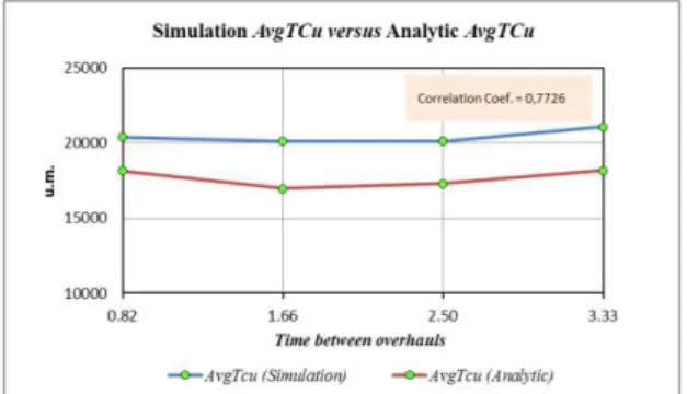
Figure 23: Comparison among the AvgTCu values estimates by the simulation model and by the analytic model (Lopes, 2007)
Finally, through Figure 23 it can be verified that the behavior of AvgTCu is identical in both models. However this results analysis lacks confirmation due to small sample size dimension.
6. CONCLUSIONS
Firstly, this paper shows how to develop an advanced simulation model, incorporating flexibility. This target would be reached by developing and incorporating new modules in our simulation tool, following past experiences found on literature (Dias et al. 2005, 2006 and Vilk et al. 2009, 2010) where the automatic generation of simulation programs enables desired model flexibility, i.e., making the model generating specific simulation programs for specific Maintenance Float Systems. This new development of our simulation model for our Maintenance Float System presents:
More flexibility
This was the main challenge for the work presented in this paper. The automatic generation of simulation models, depending on the three main maintenance system variables –M, number of active machines; L, number of maintenance crews; R, number of reserve machines. In fact, the user would just have to introduce M, L and R and, instantly, he will get the adequate simulation model to run and experiment.
More interactivity
Now the user has the possibility to interact with the simulation model during each simulation run. In fact the user can now modify all variables of the maintenance system under
analysis and can, therefore, evaluate system behaviour under different maintenance strategies.
Better information
This model now offers much better maintenance information. Indeed, the strong visual aspect offered by the developed model clarifies the actual process inside the system. This allows a better understanding of the different interactions in the model and of the simulation results.
This paper also shows that the estimated values for the performance measures analysed (system availability and total maintenance cost per time unit) present similar values for the simulation model and analytical model, as far as a Maintenance Float System with M=10, R=5 and L=5 is concerned. Also, it is quite clear that variance is different for both global efficiency measures analysed, especially when using extreme values for periodic overhauls rates. In this respect, AvgSav is the most sensitive parameter. As expected, the least sensitive parameter is AvgTCu, as it does not take into consideration the number of available machines, i.e., the cost for production loss is constant, irrespective of the number of available machines in the system.
However, the greatest overall contribution of this paper is therefore related to the construction of a flexible simulation decision support tool for MFS, where several efficiency measures of MFS are involved. Thus, in any classic MFS (number of active machines, number of spare machines and maintenance crews) subject to preventative actions and accidental actions of maintenance, this tool deals with the evaluation of its efficiency in terms of costs and in terms of availability. Also, considering simultaneously preventive maintenance actions and accidental maintenance actions, represents another novelty, once the simulation models found on the literature would approach these issues individually. Moreover, this simulation tool enables to tackle large scale float systems, up to 1000 actives machines, 1000 spare machines and 1000 maintenance crews. On the other hand, the diversity of efficiency measures calculated in the MFS simulation model really helps the decision maker to take the appropriate decisions. Finally this model presents the advantages usually associated with simulation models, namely a better understanding of the functioning of the system, the possibility of identifying the critical points of the system and the easy adaptation of the simulation model to reflect changes in the operating conditions of the system.
7. FUTURE DEVELOPMENTS
to the development of an advanced simulation model, incorporating still more flexibility. This target would be reached by developing and incorporating new modules in our simulation tool, in order to also incorporate maintenance systems where failure rates would also vary while the model runs, i.e., where a Non Homogeneous Poisson Process (NHPP) is present. These mentioned future developments also intend to potentiate the known capability of simulation to efficiently communicate with managers and decision makers, even if they are not simulation experts.
Acknowledgments. This work was funded by the "Programa Operacional Fatores de Competitividade - COMPETE" and by the FCT - Fundação para a Ciência e Tecnologia in the scope of the project: FCOMP-01-0124-FEDER-022674.
REFERENCES
Alabdulkarim A. A., Ball, P. D., Tiwari, A., 2013, Applications of simulation in maintenance research, World Journal of Modeling and Simulation, Vol. 9 (2013) No. 1, pp. 14-37.
Alam, Fasihul M.; McNaught, Ken R. and Ringrose, Trevor J., 2003, Developing Simulation Metamodels for a Maintenance Float System, AMORG, Engineering Systems Department, Cranfield University, RMCS Shrivenham, Swindon SN6 8LA, UK
Chen, M. C. and Tseng, H. Y., 2003, An approach to design of maintenance float systems, Integrated Manufacturing Systems, vol. 14, pp. 458-467.
Chen, M. and Tseng, H., 2003, An approach to design of maintenance float systems, Integrated Manufacturing Systems, vol. 14, no. 5, pp. 458-467.
Dias, Luis M. S; Rodrigues, A. J. M. Guimarães; Pereira, Guilherme A. B., 2005, An Activity Oriented Visual Modelling Language with Automatic Translation to Different Paradigms, Proceedings of the 19th European Conference On Modelling And Simulation (ECMS 2005), Riga, Letónia. Ed. Yury Mercuryev et al. Junho de 2005. pp. 452-461.
Dias, Luis S; Pereira, Guilherme A. B. and Rodrigues, A. J. M. Guimarães, 2006, A Shortlist of the Most Popular Discrete Simulation Tools, ASIM 2006 - 19th Symposium on Simulation Technique. SCS Publishing House. Ed. M. Becker and H. Szczerbicka. Hanover, Alemanha. pp. 159-163.
Dias, Luis S.; Pereira, Guilherme A. B. and Rodrigues, A. J. M. Guimarães, 2006, Activity based modeling with automatic prototype generation of process based arena models, EMSS 2006 - 2nd European Modeling and Simulation Symposium. Barcelona, Espanha. pp. 287-296.
Dias, L S, Pereira, G A B, Vik, P and Oliveira, J A V.
Discrete Simulation Tools Ranking – a Commercial Software Packages Comparison Based on Popularity. Industrial Simulation Conference, Venice, Italy, June 2011: 5-10.
Gupta, V. and Rao, T., 1996, On the M/G/1 machine interference model with spares, European Journal of Operational Research, vol. 89, pp. 164-171.
Gupta, S. M., 1997, Machine interference problem with warm spares, server vacations and exhaustive service, Performance Evaluation, vol. 29, pp. 195-211.
Kelton, W. David; Sadowski, Randall P. and Strurrok, David T., 2004, Simulation With Arena, (3rd edition), McGraw-Hill, 1998-2004.
Kuei, C. H. and Madu, C. N., 1994, Polynomial metamodelling and Taguchi designs in simulation with application to the maintenance float system, European Journal of Operational, Reseach, vol. 72, pp. 364-375.
Lopes, Isabel S., 2007, Técnicas Quantitativas no Apoio à Decisão em Sistemas de Manutenção, Tese de Doutoramento, Universidade do Minho.
Lopes, Isabel S.; Leitão, Armando L. F. and Pereira, Guilherme A. B., 2005, Modelo de Custos de Manutenção para um Sistema com M Unidades Idênticas, in C. G. Soares, A. P. Teixeira e P. Antão (eds), Análise e Gestão de Riscos, Segurança e Fiabilidade 2: p 603-620, Lisboa: Edições Salamandra (ISBN 972-689-230-9).
Lopes, Isabel S.; Leitão, Armando L. F. and Pereira, Guilherme A. B., 2006, A Maintenance Float System with Periodic Overhauls, in Guedes Soares & Zio (eds), Safety and Reliability for Managing Risk 1: p 613-618, London: Taylor & Francis Group (ISBN 0-415-41620-5).
Madu, C. N. and Kuei, C. H., 1992b, Simulation metamodels of system availability and optimum spare and repair units, IIE Transactions, vol. 24, pp. 99-104.
Madu, C. N. and Lyeu, P., 1994, On the use of simulation metamodeling in solving system availability problems, Microelectronics Reliability, vol. 34, pp. 1147-1160.
Madu, I. E., 1999, Robust regression metamodel for a maintenance float policy, International Journal of Quality & Reliability Management, vol. 16, pp. 433-456.
Pegden, C.D.; Shannon, R. E.and Sadowski, R. P., 1990 Introduction to Simulation Using SIMAN, McGraw-Hill, New York, USA. v. 2.
(ECEC 2011). London, England. pp.68-74.
Pidd, Michael, 1989, Computer Modelling for Discrete Simulation, Wiley.
Pidd, Michael, 1993, Computer Simulation in Management Science, Third Edition, Wiley. Zeng, A. Z. and Zhang, T., 1997, A queuing model for
designing an optimal three-dimensional maintenance float system, Computers & Operations Research, vol. 24, pp. 85-95.
AUTHORS BIOGRAPHY
FRANCISCO PEITO was born in 1966 in Macedo de Cavaleiros, Portugal. He graduated in Mechanical Engineering-Management of Production in Polytechnic Institute of Porto. He holds an MSc degree Industrial Maintenance in University of Porto. His main research interests are Simulation and Maintenance.
GUILHERME PEREIRA was born in 1961 in Porto, Portugal. He graduated in Industrial Engineering and Management at the University of Minho, Portugal. He holds an MSc degree in Operational Research and a PhD degree in Manufacturing and Mechanical Engineering from the University of Birmingham, UK. His main research interests are Operational Research and Simulation.
ARMANDO LEITÃO was born in 1958 in Porto, Portugal. He graduated in Mechanical Engineering at University of Porto, Portugal. He holds an MSc degree in Production Engineering and a PhD degree in Production Engineering from the University of Birmingham, UK. His main research interests are Reliability and Quality Maintenance.