SIMULATION AS A DECISION SUPPORT TOOL IN MAINTENANCE FLOAT SYSTEMS
– SYSTEM AVAILABILITY VERSUS TOTAL MAINTENANCE COST
Francisco Peito(a), Guilherme Pereira(b), Armando Leitão(c), Luís Dias(d)
(a)
Industrial Management Dpt., Polytechnic Institute of Bragança
(b)
Research Centre ALGORITMI, University of Minho
(c)
Industrial Management Dpt., Polytechnic Institute of Bragança
(d)
Research Centre ALGORITMI, University of Minho
(a)
[email protected], (b)[email protected], (c)[email protected], (d)[email protected]
ABSTRACT
This paper is concerned with the use of simulation as a decision support tool in maintenance systems, specifically in MFS (Maintenance Float Systems). For this purpose and due to its high complexity, in this paper the authors explore and present a possible way to construct a MFS model using Arena® simulation language, where some of the most common performance measures are identified, calculated and analysed. Nevertheless this paper would concentrate on the two most important performance measures in maintenance systems: system availability and maintenance total cost. As far as these two indicators are concerned, it was then quite clear that they assumed different behavior patterns, specially when using extreme values for periodic overhauls rates. In this respect, system availability proved to be a more sensitive parameter.
Keywords: Simulation, Discrete Event Simulation, Maintenance, Preventive Maintenance, Waiting Queue Theory, Float Systems.
1. INTRODUCTION
In production areas and service systems such as transport companies, health service systems and factories, the main goal is to achieve high levels of competitiveness and operational availability. In this environment the need for equipment to work continuously is very likely in order to maintain high levels of productivity. This is why MFS has an important role on equipment breakdown and production stoppage has a high and direct impact on production process efficiency.and, as a consequence, on their operational results. Therefore, maintenance control and equipment use optmization become not only an important aspect for the mentioned reasons, but also for personnel security matters and to prevent negative environmental impact.
In general, preventive maintenance implementation increases equipment control and avoids unexpected stoppages. However, to overestimate these actions makes the maintenance costs too high for the required availability.
In production systems involving identical equipments such as the float systems it is an advantage to integrate maintenance management with materials and human resources. An example of this to have spare equipment to replace those that fail or need review. Then, the direct and indirect costs due eqiupment stoppage are minimized and the level of production or service requirements fullfield. Although the existance of spare equipment is important to maintain the production process working it is recommended to keep the number of spare equipment in an optimal level for economic reasons.
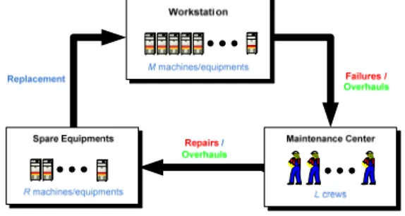
Fig. 1 –Typical Maintenance Float System
A typical Maintenance Float System is composed of a workstation, a maintenance center with a set of maintenance crews to perform overhauls and repair actions and a set of spare machines (Fig.1). The workstation consists of a set of identical machines and the repair center of a limited number of maintenance crews and a limited number of spare machines. The maintenance crew is responsible for the repair and overhaul actions and also responsible for:
a) the transportation of the spare macines from the maintenance centre wharehouse to the workstation;
b) the removal and transportation of the machines needing repair or overhaul action to the maintenance centre;
After having described the maintenance float system under consideration, the next section of this paper focus on the literature review on analytical models for this type of maintenance system, thus allowing some type of validation for the simulation results achieved.
The following section describes the simulation model developed, based on the purpose of analysing system availability and total maintenance cost.
Next, this paper includes a section for output analysis, in order to evaluate sensitivity, precision and robustness of both performance measures under consideration.
Conclusions and Further Developments are the closing sections for this paper.
2. RESEARCH BACKGROUND
As far as float systems maintenance models is concerned, (Lopes 2007) refers some studies where simulation has been used to produce results based on specified parameters. Due to the fact that these simulation models were only concerned with the input/output process, without dealing with what is happening during the simulation data process, some metamodels have emerged (Madu and Kuei 1992a; Madu and Kuei 1992b; Madu and Lyeu. 1994; Kuei and Madu 1994; Madu 1999; Alam et al. 2003). The metamodels express the input/output relationship through a regression equation. These metamodels can also be based on taguchi methods (Madu and Kuei 1992a; Kuei and Madu 1994) or on neuro networks (Chen and Tseng 2003). These maintenance system models were also recently treated on an analytical basis by (Gupta and Rao 1996; Gupta 1997; Zeng and Zhang 1997; Shankar and Sahani 2003; Lopes 2007). However, the model proposed by (Lopes 2007) is the only one that deals, simultaneously, with three variables: number of maintenance teams, number of spare equipments, and time between overhauls, aiming the optimization of the system performance. Although this proposed model already involves a certain amount of complexity it may become even more complex by adding new variables and factors such as: a) time spent on spare equipment transportation, b) time spent on spare equipment installation; c) the introduction of more or different ways of estimating efficient measures; d) allowing the system to work discontinuously; e) speed or efficiency of the repair and revision actions; f) taking into account restrictions on workers timetable to perform the repair and revision actions; g) taking into account the workers scheduling to perform the repair and revision actions; h) taking into account the possibility of spare equipment failure; etc. Anyway these mentioned approaches would aim at ending up with MFS models very close to real system configurations. In fact, the literature review showed that most of the works published, involving either analytical or simulation models, concentrate on a single maintenance crew, or on a single machine on the
workstation or even considering an unlimited maintenance capacity – thus overcoming the real system complexity and therefore not quite responding to the real problem as it exists.
As far as the model presented by (Lopes et al. 2005; Lopes et al. 2006; Lopes 2007) is concerned it is assumed that systems works continuously, its availability is not calculated and the system optimazation is only based on the total maintenance cost per time unit. Moreover, it considers that the total system maintenance cost is the same without taking into account the number of machines unavailable, which in many real situations it is not the best option. Finally the referred analytical model only allows that its failures occur under an homogeneous Poisson process (HPP).
Another important aspect on the companies management strategic definition is to have their tasks correctly planned. To help this planning procedure it is important to know different indicators such as: machine availability, equipment performance and maintenance costs, among others. Therefore one should consider new factors that affect these float systems indicators: possibility of some machine failure, efficiency, repair time.
Moreover, when preventive maintenance policy is used, the time for individual replacement is smaller than time for group replacement. It means that the latter situation requires more machine on the process to be stopped, and also implies an increase for a certain time, on the maintenance crews.
In general companies policy lies on using economic models to define their best strategies. Profits maximization or costs minimization are the most frequent goals used. However, strictly from the maintenance point of view availability is frequently used as an efficient measure of the system performance, and sometimes more important than the cost based process. In this work availability is calculated dividing the time the system is up (Tup) by the time the system is up plus the time the system is down (Tdown) for maintenance reasons. Some authors, however, calculate availability through the ratio between MTBF and [MTBF+MTTR ]. Being, MTBF the-Mean Time Between Failures and MTTR the Mean Time To Repair.
3. THE SIMULATION MODEL
The Arena® simulation language environment was chosen for the development of the simulation model for this MFS (Kelton 2004; Pidd 1989; Dias et. al 2006 and Pidd 1993).
continuously. Machines that fail are taken from the workstation and sent to the maintenance park waiting queue, where they will be assisted according to arrival time. Machines that reach their optimal overhaul time are kept in service until the end of a period T without failures. However they will be also kept on a virtual queue to overhaul. If the number of failed machines plus the number of machines requiring overhaul is lower than the number of maintenance crews available, machines are replaced and repaired according to FIFO (First In First Out) rule. Otherwise if it exceeds the number of maintenance crews, the machines will either be replaced (while there are spare machines available) or will be sent to the maintenance queue. The machines that complete a duration period T or time between overhauls in operation without failures are maintained active in the workstation, where they wait to be assisted, and they are replaced when they are retired of the workstation to be submitted to a preventive intervention. Its replacement is assured by the machine that leaves the maintenance center in the immediately previous instant. If an active machine happens to fail it awaits for the accomplishment of an overhaul, then it will be immediately replaced, if a spare machine is available or as soon it is available.
Furthermore the time to replace a machine that needs overhaul or has failed is also included in our model and this is a parameter that could be adjusted during a simulation run.
In the MFS here analized, it is assumed that the M active machines of the workstation have a constant failure rate (Francisco et al. 2011). Moreover time between failures are assumed as independent and identically distributed following an Exponential Distribution for all machines (failures occur under a Homogeneous Poisson Process). However, during a simulation run, this value could be adjusted based on time between overhauls. Obviously a smaller time between overhauls implies greater time between failures.
In this first version of the simulation model the time between overhauls could be adjusted during a simulation run.
As far as time to overhaul and time to repair are concerned, we have assumed the Erlang-2 distribution, eventhough considering overhaul time significantly lower than the repair time.
For this MFS, the following three parameters and ten relevant variables are identified:
Parameters
1. Number of active machines (M);
2. Number of maintenance crews (L); 3. Number of spare machines (R);
Variables
4. Machine- Overhauls rate (λrev)*;
5. Machine-Initial Failures rate (λf)*;
6. Crews-Repair rate (µrep)*;
7. Crews-Overhaul rate (µrev)*;
8. Failure cost (Cf);
9. Repair cost (Crep);
10. Overhaul cost (Crev);
11. Replacement cost (Cs);
12. Cost due to loss production (Clp);
13. Holding cost per time unit (h); 14. Labour cost per time unit (k);
15. Time to convey and install spare machine
(TConvInst).
(*) This variable can be adjusted during the simulation run.
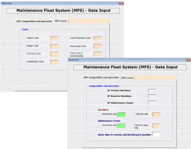
The different types of input mentioned above occur in specific developed input menus – Visual Basic for Applications within Arena model.
Fig. 2 - Data input area sample screenshot
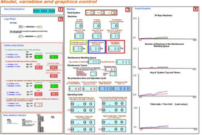
Figures 2 and 3 highlight both input variables window and output updates – numerically and graphically. Fig. 4 shows an application screenshot including simulation animation.
The developed simulation application for a Maintenance Float System allows the estimation of the following global efficiency measures:
a) Average system availability (AvgSAv);
b) Total maintenance cost per time unit [(AvgTCu) and AvgTCu(*)].
Total Maintenance Cost per Time Unit would be estimated in two different ways:
Fixed cost, independent of the number of available machines in the system;
Fig. Fig. 4 Howeve be estimated, c) Ave wor d) Ave mai e) Ave wait f) Ave g) Prob Mac h) Prob (Pro And, fin some individ maintenance i) Util j) Util
3 - Variables
– Animation
er, some othe , such as:
erage number rkstation (AvgM erage numbe
ntenance wait erage waiting ting queue (A erage operatin bability of chines (Probim
bability of th obs);
nally, the sim dual efficienc
crew, i.e.:
lization rate pe lization rate pe
and graphics
area sample s
er performanc
r of missing m gMeq),
er of mac ting queue (Av g time in th
vgWt); ng cycle time (
existing 1
m);
he system bein
mulation mode cy measures er machine; er maintenanc control screenshot
ce measures c
machines at t
chines in t vgLq); he maintenan
(AvgD); or more id
ng fully acti
el also comput per machine ce crew; can the the nce dle ive utes or pe av (a 3. F F va Av re re (F re 4. B pr te ef Si hy ( di k) Numb perform l) Averag This pap erformance m vailability and
Simulation approximately
500 hours.
Fig. 5 – Outco number
Fig. 6 – Outco number in
For each ariables, the vgTCu and A eplications – f esults robustn Figures 5 and equired to run
. SIMULAT
earing in m reviously refe st and estim fficiency meas imulation m ypothetical s
rev). These d ifferent times
20000,00 20500,00
1 5 10
u.
m.
Outcome of
14350,00 14850,00
1 5 10
u.
m.
Outcome of t
er of overh med per main ge availability
er will focu measures men d total mainten
n length wa one year) – w
ome of the var in AvgTCu an
ome of the var n AvgTCu(*) a
set of input p simulation o AvgTCu(*) we
for an adequat ness for bot
6) and also d the model.
TION RESUL
mind the tw erred, simulat mate the beha sures mention odels were cenarios with different review between revi 20175,46 50,46
15 20 25 30 35 40
Number of Rep
f the variation of the Replicatio
Avg TCu
14528,39 50,46
15 20 25 30 35 40
Number of Rep
the variation of the Replicatio
Avg TCu (*)
hauls and re ntenance crew
y per machine
us on the ntioned abov nance cost per was set to warm-up peri
riation of the R nd AvgSAv var
riation of the R and AvgSAv v
parameters an output variab ere estimated ate system stab th performan
due to compu
LTS AND DI
welve variabl tion models w aviour of the ned on the pre
carried out th different w rates are as iew (T) whic
45 50 60 70 80 100
plications
ons number in Avg TCu and Avg
Avg SAv
45 50 60 70 80 100
plications
ns number in Avg TCu(*) and
Avg SAv
epair actions ;
e.
two general ve – system r time unit.
9.000 hours iod was set to
Replications riables
Replications variables
nd pattern for bles AvgSAv, based on 25 bilization and nce measures utational time
ISCUSSION
les of MFS were used to e two global vious section. t for (1-60) review rates ssociated with h are defined
20165,33 50,45 50,00 50,50 51,00 110 120
g SAv
Rta e 14530,27 50,45 50,00 50,50 51,00 110 120
Avg SAv
accordingly to the preventive maintenance policy aiming the best option.
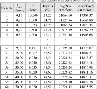
Table 1- Global efficiency measures outcomes in the MFS model after 25 replication
(Values estimated by simulation after 25 replication)
S c e n a r i o λrev
(/hour)
T
(hour)
AvgSAv
(%)
AvgTCu
(m.u./hour)
AvgTCu(*)
(m.u./hour)
1 0,10 10,000 29,25 21064,60 17304,37
2 0,20 5,000 34,75 21127,96 16646,80
3 0,30 3,333 40,79 21065,24 15870,35
4 0,40 2,500 45,26 20915,39 15287,79
5 0,50 2,000 48,12 20751,46 14908,68
. . .
. . .
. . .
. . .
. . .
. . .
52 9,00 0,111 48,71 20195,00 14776,87 53 15,00 0,067 48,52 20212,24 14807,21 54 20,00 0,050 48,54 20228,63 14815,57 55 25,00 0,040 48,56 20223,63 14814,18 56 30,00 0,033 48,54 20230,24 14816,98 57 35,00 0,029 48,62 20226,82 14811,16 58 40,00 0,025 48,54 20229,16 14820,31 59 45,00 0,022 48,50 20228,80 14822,78 60 50,00 0,020 48,52 20226,42 14815,55
(*)Considers that the cost of lost production changes in function of the number of active
machines lacking in the system.
Table 2 – Observe percentual change in the global efficiency measures after 25 replication
MPO -Observe percentual change
S c e n a r i o AvgSAv AvgTCu AvgTCu(*)
1-2 15,83% 0,30% -3,95% 2-3 14,80% -0,30% -4,89% 3-4 9,87% -0,72% -3,81% 4-5 5,95% -0,79% -2,54%
. . .
. . .
. . .
. . .
52-53 -0,14% 0,06% 0,10%
. . .
. . .
. . .
. . .
58-59 -0,07% 0,00% 0,02%
59-60 0,04% -0,01% -0,05%
Max. 15,83% -0,79% -4,89%
Mean 0,80% -0,07% -0,27%
A first global analysis of the values prsented in tables 1 and 2 indicate that the precision obtained on the three efficient measures analysied is different. An individual analysis of each meaure indicates that AvgTCtu shows the smaller variation (MPO lower). In Table 1 it can also be observed that when T takes very small values (T≤0.111 or λrev≥ 9) the three efficient
measures [AvgTCtu, AvgTCTu(*) and AvgSAv] are kept practically unchangeable. This fact can be confirmed in Fig. 7 or in Table 2 where the MPO for these values of T is extremely low, almost zero. On the other hand, when T assumes very high values (T≥2,5 or
λrev≤ 0,4) the efficiency measures AvgTCTu(*) and
AvgSAv present high MPO values in opposition to AvgTCtu that shows very small values. In Table 2 it
can also be observed that AvgTCtu presents the lowest MPO average value of the three efficiency measures and that AvgSAv has the highest value.
In order to simplify the interpretation and analysis of these global efficiency measures, figures 7, 8 and 9 pinpoint the maximum and minimum values (table 2 and 3) as well as other points considered relevant for the analysis.
Table 3 - Maximum values of the main efficiency measures
Statistics
(Maximum) (/hour) λrev
T
(hour)
AvgSAv
(%) 50,70% 0,90 1,111
AvgTCu
(m.u./hour) 21127,96 0,20 5,000
AvgTCu (*)
(m.u./hour) 17304,37 0,10 10,000 Note: Red points in the graphics
Table 4 - Minimum values of the main efficiency measures
Statistics
(Minimum) (/hour) λrev
T
(hour)
AvgSAv
(%) 29,25% 0,10 10,000
AvgTCu
(m.u./hour) 20096,90 1,80 0,556
AvgTCu (*)
(m.u./hour) 14518,77 1,20 0,833 Note: Yellow points in the graphics
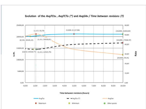
Tables 3 and 4 show that the T value corresponding to the minimum value of AvgSAv corresponds the maximum value, as expected, of AvgTCu(*). When compared with the minimum of AvgTCu, there is a significant T gap ( 5 hours), although, its remains practically the same when the value of T changes from 5 to 10 hours (Fig. 9).
When comparing the T value corresponding to the maximum value of AvgSAv with the T value corresponding to the minimum value of AvgTCu(*), there is only a small gap, which is clearly higher in the case of the T value orresponding to the minimum of the AvgTCu (Fig. 9)
Table 5- Correlation coefficients
T AvgSav AvgTcu AvgTcu(*)
T 1 -0,9021 0,8279 0,9017
AvgSav -0,9021 1 -0,7980 -0,9986
AvgTcu 0,8279 -0,7980 1 0,8237
AvgTcu (*) 0,9017 -0,9986 0,8237 1
AvgTCu(*) (99,8%). However when AvgTCu is compared with AvgTCu(*) or with AvgSav, the correlation coefficient decreases to 82,37% and to 79,80%, respectively. This partially explains why in tables 3 and 4 the T value corresponding to the maximum of AvgSav does nor correspond exactly to the T value corresponding to the minimum of the AvgTCu and AvgTCu(*) and that difference being higher in the case of AvgTCu(*) (Fig. 9).
Fig. 7 - Evolution of the AvgTCtu, AvgTCTu(*) and AvgSAv / Revision rate (λrev)
Fig. 8.Evolution of the AvgTCtu, AvgTCTu(*) and AvgSAv / Revision rate (λrev) [Zoom Fig.7]
Fig. 9- Evolution of the AvgTCtu, AvgTCTu(*) and AvgSAv / Time between revisions (T)
As it can be observed in Fig.7 and more clearly in figures 8 and 9, for the MFS analysed, the three global measures of efficiency being studied only present small variations for values of rev between 0,10 and 9,00 (or
T between 10,000 and 0,111 hours). For values of rev
higher than 9.00 the three global measures of efficiency remain practically unchanged.
Table 6 - Comparison among the AvgTCu values estimates by the simulation model and analytic model
(Lopes, 2007)
T Model AvgTCu (m.u./hour)
AvgTCu(*) (m.u./hour)
Δ1 (%)
Δ2 (%)
Δ3 (%)
1,66 Simulation 20381,74 14554,5 -40% -12% -25%
Analytic 18130,56 ---- ----
3,33 Simulation 20126,65 14555,62 -38% -19% -17%
Analytic 16968,39 ---- ----
1,66 Simulation 20111,24 14628,02 -37% -16% -18%
Analytic 17303,65 ---- ----
3,33 Simulation 21065,24 15870,35 -33% -16% -14%
Analytic 18167,34 ---- ----
mean -37% -16% -18%
Note: M=10; R=5; L=5.
(*) Considers that the cost of lost production changes in function of the number of active
machines lacking in the system.
Δ1 – Difference among Simulation AvgTCu and Simulation AvgTCu(*)
Δ2 – Difference among Simulation AvgTCu and Analytic AvgTCu
Δ3 – Difference among Analytic AvgTCu and Simulation AvgTCu(*)
Fig. 10 - Comparison among the AvgTCu values estimates by the simulation model and by the analytic
model (Lopes, 2007)
In Table 6 there is a comparison between the values obtained from the simulation model developed by the authors in a former (Peito et al 2011) and the analytical model developed by (Lopes 2007). The sample size of the results presented and compared in this case was limited by the number of results presented by the author in her work (Lopes, 2007) . In this table it can be verified that when the two global efficiency measures are both estimated from the simulation model the difference (Δ1) is on average
-37%, presenting AvgTCu always higher values. However when AvgTCu is estimated through the analytical model that difference (Δ3) is on average
-18%. When the same efficiency global measure based on the analytical model is compared with the one calculated based on the simulation model, AvgTCu, this
(0,20; 21127,96)
(0,90; 20318,01) (1,80; 20096,90)
(0,10; 17304,37)
(0,90; 14525,79) (1,20; 14518,77) (0,90; 50,70)
0,00 10,00 20,00 30,00 40,00 50,00 60,00
0,00 5000,00 10000,00 15000,00 20000,00 25000,00
0,100 5,100 10,100 15,100 20,100 25,100 30,100 35,100 40,100 45,100 50,100
u.
m
.
Ra
te
Evolution of the AvgTCtu , AvgTCTu (*) andAvgSAv / Revision rate (λrev)
AvgTcu AvgTcu (*) AvgSav
Revision rate
Maximum Minimum Other points
(0,20; 21127,96)
(0,90; 20318,01) (1,80; 20096,90) (0,10; 17304,37)
(0,90; 14525,79) (1,20; 14518,77)
(0,10; 29,25) (0,90; 50,70)
0,00 10,00 20,00 30,00 40,00 50,00 60,00
0,00 5000,00 10000,00 15000,00 20000,00 25000,00
0,020 2,020 4,020 6,020 8,020 10,020
u.
m
.
Ra
te
Evolution of the AvgTCtu , AvgTCTu(*) andAvgSAv / Revision rate (λrev)
AvgTcu AvgTcu (*) AvgSav
Revision rate
Maximum Minimum Other points
(10,000; 21064,60) (5,000; 21127,96)
(1,111; 20318,01)
(0,526; 20105,22) (10,000; 17304,37)
(1,111; 14525,79) (0,833; 14518,77)
(10,000; 29,25) (1,111; 50,70)
0,00 10,00 20,00 30,00 40,00 50,00 60,00
0,00 5000,00 10000,00 15000,00 20000,00 25000,00
0,020 1,020 2,020 3,020 4,020 5,020 6,020 7,020 8,020 9,020 10,020
u.
m
.
Ra
te
Evolution of the AvgTCtu , AvgTCTu (*) andAvgSAv / Time between revisions (T)
AvgTcu AvgTcu (*) AvgSav
Time between revisions (hours)
Maximum Minimum Other points
0 5000 10000 15000 20000 25000
0,82 1,66 2,50 3,33
u.
m
.
SimulationAvgTCu versus AnalyticAvgTCu
AvgTcu (S) AvgTcu (A)
Time between revisions
if calculated from the analytical model presents lower values, on average, of 16%. It is also observed that the analytical model always presents for its efficiency measure values that lie between the two efficiency measures estimated from the simulation model.
Finally, through Fig. 10 it can be verified tha the behaviour of AvgTCu is identical in both models. However this results analysis lacks confirmation due to small sample size dimension.
5. CONCLUSIONS
This paper shows similar estimated values for the performance measures analysed – system availability and total maintenance cost per time unit, for both simulation model and analytical model, as far as a Maintenance Float System with M=10, R=5 and L=5 is concerned. Nevertheless a difference of nearly 15% is noticed. Also, it is quite clear that variance is different for both global efficiency measures analysed, specially when using extreme values for periodic overhauls rates. In this respect, AvgSav is the most sensitive parameter. As expected, the least sensitive parameter is AvgTCu , as it does not take into consideration the number of available machines, i.e., the cost for production loss is constant, irrespective of the number of available machines in the system.
6. FUTURE DEVELOPMENTS
The simulation model here presented, incorporating analysis of usual performance measures, also drives its concern towards new efficiency measures, enabling new trends for the analysis and discussion of the best decisions as far as a specific Maintenance Float System is concerned. Nevertheless the authors are now aiming to the development of an advanced simulation model, incorporating flexibility. This target would be reached by developing and incorporating new modules in our simulation tool, following past experiences found on literature (Luís S Dias, 2005, 2006 and Vilk, P., 2009, 2010) where the automatic generation of simulation programs enables desired model flexibility, i.e., making the model generating specific simulation programs for specific Maintenance Float Systems. These mentioned future developments also intend to potentiate the known capability of simulation to efficiently communicate with managers and decision makers, even if they are not simulation experts.
REFERENCES
Alam, Fasihul M.; McNaught, Ken R. and Ringrose, Trevor J. (2003), “Developing Simulation Metamodels for a Maintenance Float System”, AMORG, Engineering Systems Department, Cranfield University, RMCS Shrivenham, Swindon SN6 8LA, UK
Chen, M. C. and Tseng, H. Y. (2003), "An approach to design of maintenance float systems," Integrated Manufacturing Systems, vol. 14, pp. 458-467.
Dias, Luis M. S; Rodrigues, A. J. M. Guimarães; Pereira, Guilherme A. B. (2005), An Activity Oriented Visual Modelling Language with Automatic Translation to Different Paradigms, Proceedings of the 19th European Conference On Modelling And Simulation (ECMS 2005), Riga, Letónia. Ed. Yury Mercuryev et al. Junho de 2005. pp. 452-461
Dias, Luis S; Pereira, Guilherme A. B. and Rodrigues, A. J. M. Guimarães (2006), “A Shortlist of the Most ‘Popular’ Discrete Simulation Tools”, ASIM 2006 - 19th Symposium on Simulation Technique. SCS Publishing House. Ed. M. Becker and H. Szczerbicka. Hanover, Alemanha. pp. 159-163.
Dias, Luis S.; Pereira, Guilherme A. B. and Rodrigues, A. J. M. Guimarães (2006), “Activity based modeling with automatic prototype generation of process based arena models”, EMSS 2006 - 2nd European Modeling and Simulation Symposium. Barcelona, Espanha. pp. 287-296
Gupta, V. and Rao, T. (1996), "On the M/G/1 machine interference model with spares," European Journal of Operational Research, vol. 89, pp. 164-171.
Gupta, S. M. (1997), "Machine interference problem with warm spares, server vacations and exhaustive service," Performance Evaluation, vol. 29, pp. 195-211.
Ingalls, Ricki G. (2001), "Introduction to Simulation", in Proceedings of 2001 Winter Simulation Conference, B.A. Peters, J.S. Smith, D.J. Medeiros, and M. W. Rohrer, eds.
Kelton, W. David; Sadowski, Randall P. and Strurrok, David T. (2004), "Simulation With Arena", (3rd edition), McGraw-Hill, (1998-2004).
Kuei, C. H. and Madu, C. N. (1994), "Polynomial metamodelling and Taguchi designs in simulation with application to the maintenance float system," European Journal of Operational, Reseach, vol. 72, pp. 364-375.
Lopes, Isabel S. (2007), "Técnicas Quantitativas no Apoio à Decisão em Sistemas de Manutenção", Tese de Doutoramento, Universidade do Minho. Lopes, Isabel S.; Leitão, Armando L. F. and Pereira,
Guilherme A. B. (2005), "Modelo de Custos de Manutenção para um Sistema com M Unidades Idênticas", in C. G.Soares, A. P. Teixeira e P. Antão (eds), Análise e Gestão de Riscos, Segurança e Fiabilidade 2: p 603-620, Lisboa: Edições Salamandra (ISBN 972-689-230-9). Lopes, Isabel S.; Leitão, Armando L. F. and Pereira,
Guilherme A. B. (2006), "A Maintenance Float System with Periodic Overhauls", in Guedes Soares & Zio (eds), Safety and Reliability for Managing Risk 1: p 613-618, London: Taylor & Francis Group (ISBN 0-415-41620-5).
of multi-echelon maintenance float simulation metamodels," Computers and Operations Research vol. 19, pp. 95-105.
Madu, C. N. and Kuei, C. H. (1992b), "Simulation metamodels of system availability and optimum spare and repair units," IIE Transactions, vol. 24, pp. 99-104.
Madu, C. N. and Lyeu, P. (1994), "On the use of simulation metamodeling in solving system availability problems," Microelectronics Reliability, vol. 34, pp. 1147-1160.
Madu, I. E. (1999), "Robust regression metamodel for a maintenance float policy," International Journal of Quality & Reliability Management, vol. 16, pp. 433-456.
Mamede, Nuno (1984), "Simulação Digital de Processos", Tese de Mestrado em Engenharia Electrotécnica e de Computadores (Telecomunicações e Computadores), Instituto Superior Técnico.
Pegden, C.D.; Shannon, R. E.and Sadowski, R. P. (1990) "Introduction to Simulation Using SIMAN, McGraw-Hill", New York, USA. v. 2. 1990.
Pidd, Michael (1989), "Computer Modelling for Discrete Simulation", (Editor), Wiley.
Pidd, Michael (1993), "Computer Simulation in Management Science", Third Edition, Wiley. Peito, Francisco; Pereira, Guilherme; Leitão, Armando;
Dias, Luís (2011), “Simulation as a Decision Support Tool in Maintenance Float Systems” ,17th European Concurrent Engineering Conference (ECEC´2011). London, England. pp.68-74.
Rodrigues, Guimarães and Carvalho, Valério (1984), "CAPS - ECSL, Experiência de modelagem e simulação aplicada a um sistema de elevadores", Relatório Técnico, Universidade do Minho.
Rubinstein, Reuven Y. and Melamed, Benjamin (1998), "Modern Simulation and Modeling", Wiley Series in Probability and Statistics, Applied Probability and Statistics Section, A Wiley-Interscience Publication, John Wiley & Sons, INC., ISBN 0- 471-17077-1.
Shannon, Robert E. (1998), "Introduction to the Art and Science of Simulation", in Proceedings of 1998 Winter Simulation Conference, D.J.Medeiros, E.F. Watson, J.S. Carson and M.S. Manivannan, eds.
Shankar, G. and Sahani, V. (2003), "Reliability analysis of a maintenance network with repair and preventive maintenance," International Journal of Quality & Reliability Management, vol. 20, pp. 268-280.
Vik, P.; Pereira, G. and Dias, L. (2009), “Software Tools Integration for the Design of Manufacturing Systems”, Proceedings of the Industrial Simulation Conference, Loughborough, eds. Diganta Bhusan Das, Vahid Nassehi and Lipika Deka, pp 127-131
Vik, P.; Dias, L. and Pereira, G. (2010), “Automatic Generation of Computer Models Through the Integration of Production Systems Design Software Tools”. ASMDO2010 - Third International Conference on Multidisciplinary Design Optimization and Applications. Paris (France)
Vik, P.; Dias, L.; Pereira, G. and Oliveira, J. (2010), “Improving Production and Internal Logistics Systems – An Integrated Approach Using CAD and Simulation”. ILS2010 - 3rd International Conference on Information Systems, Logistics and Supply Chain - Creating value through green supply chains. Casablanca (Morocco), April 14-16.
Zeng, A. Z. and Zhang, T. (1997), "A queuing model for designing an optimal three-dimensional maintenance float system", Computers & Operations Research, vol. 24, pp. 85-95.
AUTHOR BIOGRAPHY
FRANCISCO PEITO was born in 1966 in Macedo de Cavaleiros, Portugal. He graduated in Mechanical Engineering-Management of Production in Polytechnic Institute of Porto. He holds an MSc degree Industrial Maintenance in University of Porto. His main research interests are Simulation and Maintenance.
GUILHERME PEREIRA was born in 1961 in Porto, Portugal. He graduated in Industrial Engineering and Management at the University of Minho, Portugal. He holds an MSc degree in Operational Research and a PhD degree in Manufacturing and Mechanical Engineering from the University of Birmingham, UK. His main research interests are Operational Research and Simulation.
ARMANDO LEITÃO was born in 1958 in Porto, Portugal. He graduated in Mechanical Engineering at University of Porto, Portugal. He holds an MSc degree in Production Engineering and a PhD degree in Production Engineering from the University of Birmingham, UK. His main research interests are Reliability and Quality Maintenance.