Small area estimation for the price of habitation transaction: comparison of different uncertainty measures of temporal EBLUP

Texto

(1)Proceedings of Q2008 European Conference on Quality in Official Statistics. Small area estimation for the price of habitation transaction: comparison of different uncertainty measures of temporal EBLUP Luís N. Pereira, ESGHT – Universidade do Algarve1 Pedro S. Coelho, ISEGI – Universidade Nova de Lisboa. 1. Introduction Local level planning requires reliable statistics for small areas, but normally due to cost or logistic constraints, sample surveys are often planned to provide reliable estimates only for large geographical regions and large subgroups of a population. As a result, many domains of interest can be unplanned at the design stage and the sample sizes in these domains are rarely large enough to provide adequate precision for direct domain estimators. For example, data from the Prices of the Habitation Transaction Survey (PHTS) in Portugal only allows the production of reliable direct estimates for the mean price of habitation transaction for the country and for large geographical regions, like NUTSII (NUTS stands for the “Nomenclature of Territorial Units for Statistics” which is defined by the regulation EC No 1059/2003 of the European Parliament). In fact, the PHTS sample sizes are very small or even zero in many other domains of interest (e. g. NUTSIII, municipalities). For these unplanned small areas with small sample sizes, traditional direct estimators are either not feasible or provide unacceptably large variation coefficients. This creates the need to employ indirect estimators that “borrow information” from related small areas and time periods through linking models, using recent census and current administrative data, in order to increase the effective sample size and thus precision. Several indirect small area estimators based on explicit linking models have been proposed in recent years. For a review of indirect small area estimators, we refer to the book by Rao (2003). In this paper, it is assumed that the small area parameters of interest follow a Rao-Yu longitudinal model (Rao and Yu, 1994) in order to combine information from longitudinal surveys and related auxiliary variables. The Rao-Yu model is a crosssectional and time-series stationary area level model involving autocorrelated random effects and sampling errors with an arbitrary covariance matrix over time, and using analysis of variance (ANOVA) estimates of variance components. In fact, this model is a special case of the general linear mixed model (LMM) involving autocorrelated random effects with a homogeneous covariance structure (first-order autoregressive plus common covariance: AR(1)+J). Under this model, the empirical 1. Address for correspondence: Luís N. Pereira, Escola Superior de Gestão, Hotelaria e Turismo – Universidade do Algarve, Campus da Penha, 8005-139 Faro, Portugal (Lmper@ualg.pt).. 1.

(2) best linear unbiased prediction (EBLUP) approach is used for the estimation of small area parameters of interest. While EBLUP estimators are fairly easy to obtain under the Rao-Yu model, measuring its quality is a challenging problem due to difficulties on estimating the mean squared prediction error (MSPE) of such estimators. Nevertheless, estimation of the MSPE of the EBLUP is of significant practical interest. Therefore, research on estimation of MSPE of EBLUP in small area estimation problems has received a considerable attention in recent years. See Rao (2003) and Jiang and Lahiri (2006) for a review of MSPE estimation. The aim of this paper is to compare different uncertainty measures of the small area estimator based on the Rao-Yu model, using real data from the PHTS conducted by the Portuguese Statistical Office. The paper is organized as follows. Section 2 reviews the cross-sectional and timeseries stationary area level model due to Rao and Yu (1994) and describes how the EBLUP is obtained. Different MSPE estimators of the temporal EBLUP are presented in section 3. In the framework of an application with real data, section 4 addresses both the estimates of mean price of the habitation transaction and a comparison of different uncertainty measures of these estimates. Finally, the paper ends with a conclusion in section 5.. 2. The Rao-Yu model In order to take advantage of the chronological nature of data, Rao and Yu (1994) proposed the following area specific model: θît = θ it + eit ,. (1). θ it = x′it β + vi + uit , u it = ρu i ,t −1 + ε it ,. ρ < 1,. (2). where θ it is the parameter of inferential interest for the ith small-area at tth time point (i=1, …, m; t=1, …, T) and θˆ is its design-unbiased direct survey estimator (based it. only on the sample from the ith small-area at tth time point), eit ’s are independent sampling errors normally distributed, given the θ it ’s, with mean 0 and known variance. σ it2 , x it = ( xit1 ,..., xitp )′ (p×1) is a column vector of an area-by-time specific auxiliary variables and β (p×1) is a column vector of regression parameters. Further, vi ’s are iid. (. ). random area specific effects with v i ~ N 0, σ v2 and u it ’s are random area-by-time specific effects following a common AR(1) process for each i, with ε it ~ N (0, σ 2 ). The iid. random effects, vi and u it , represent the area and the area-by-time characteristics not accounted by the auxiliary variables. The constant ρ is a measure of the level of temporal autocorrelation. The errors {eit }, {vi } and {u it } are assumed to be mutually 2.

(3) independent. Combining the sampling error model (1) with the linking model (2), Rao and Yu (1994) obtained the following stationary small area model:. θît = x′it β + vi + uit + eit , uit = ρui ,t −1 + ε it ,. ρ < 1.. (3). Note that the well-known Fay-Herriot model (Fay and Herriot, 1979) may be obtained from model (3) setting T = 1 , ρ = 0 and σ 2 = 0 . Rao and Yu (1994) applied a special form of the model (3) assuming eit ~ N (0,1) . They showed that the model (3) can be expressed in matrix form as: iid. θˆ = Xβ + Zv + u + e ,. (4). where θˆ = col1≤i ≤ m (θˆ i ) , θˆ i = col1≤t ≤T (θît ) , X = col1≤i ≤ m (X i ) , X i = col1≤t ≤T (x′it ) , Z = I m ⊗ 1T , v = col1≤i ≤m (vi ) , u = col1≤i ≤ m (u i ) , u i = col1≤t ≤T (u it ) , e = col1≤i ≤ m (e i ) , e i = col1≤t ≤T (eit ) , I m is the identity matrix of order m and 1T (T×1) is a column vector of 1’s. Further, e , v and u are mutually independent, with u ~ N (0, σ 2 I m ⊗ Γ ) , v ~ N(0,σv2Im ) and. e ~ N (0, R ) , where Γ (T×T) is the matrix with elements ρ. i− j. (1 − ρ ) and 2. R = diag1≤i ≤ m;1≤t ≤T (σ it2 ) . Assuming that eit ~ N (0,1) , we can now see that the model (4) is a special case of the general LMM with block-diagonal homogeneous covariance structure, Cov(θˆ ) = V = block diag1≤i ≤m (Vi ) with Vi = σ 2 Γ + σ v2 J T + I T . Assuming iid. ψ = (σ v2 , σ 2 , ρ ) ′ is known, the BLUP estimator of θ it is given by:. ~. ~. ~. θ it (ψ ) = x ′it β + (σ v2 1T + σ 2 γ t ) ′Vi−1 (θˆ i − X i β ) ,. (. ~ where β = X′V −1 X. (5). ). −1. X ′V −1 θˆ is the generalized least squares estimator of β and γ t is the tth row of Γ . In practice, ψ is unknown and is estimated from the data. Let ψˆ be ( a consistent estimator of ψ . Then, an empirical BLUP of θ it , say θ it (ψˆ ) , is obtained ~ from θ it (ψ ) with ψ replaced by ψˆ . Rao and Yu (1994) provided method of moments estimators of σ v2 and σ 2 , through an extension of Henderson method 3 (Henderson, 1953), and proposed a naïve estimator of ρ . However, their main research focused on derivation of an EBLUP estimator of θ it and an estimator of its MSPE, assuming known ρ. Thus, from this ′ point forward we define the vector of variance components as ψ = σ v2 ( ρ ), σ 2 ( ρ ) .. [. ]. 3. Uncertainty measures of temporal EBLUP While the temporal EBLUP is fairly easy to obtain, the estimation of its uncertainty is a challenging problem due to the variability caused by the estimation of the variance components. A naïve measure of uncertainty of the temporal EBLUP can be obtained from: 3.

(4) [. ]. ( ˆ ) = g1it (ψˆ ) + g 2it (ψˆ ) . mspeitN θ it (ψ. (6). where the terms g1it (ψ ) , which measures the uncertainty of the EBLUP due to the. estimation of the random effects, and g 2it (ψ ) due to the estimation of the fixed effects, can be found in Rao and Yu (1994).. However, in practical applications this estimator could underestimate the true MSPE, ( especially in cases where θ it (ψˆ ) varies with ψ to a significant extent and where the variability of ψˆ is not small. Fortunately, the difficult problem of estimating the MSPE of EBLUP estimators, taking the variability of the estimated variance components into account, has been faced in the small area literature by adopting different approaches. A well known general method is based on the Taylor series expansion of MSE under normality and valid for a general longitudinal linear mixed model (Prasad and Rao 1990; Datta and Lahiri 2000, Das et al. 2004). More recently, due to the advent of high-speed computers, resampling methods have been proposed under a general longitudinal LMM. Jiang et al. (2002) introduced a unified jackknife method, which is also valid for nonnormal and nonlinear mixed models and for M-estimators of model parameters, while Butar and Lahiri (2003) proposed a parametric bootstrap method based on the assumption of normality. Both resampling-based methods are applicable for various methods of estimating the variance components and are analytically less onerous than the Taylor series method. Furthermore, all these approaches are second order accurate. Under normality assumptions of both the random effects and the random errors, an analytical estimator of the MSPE of temporal EBLUP under the Rao-Yu model is given by (Rao and Yu, 1994): ( ˆ ) = g1it (ψˆ ) + g 2it (ψˆ ) + 2 g 3it (ψˆ ) . mspeitRY θ it (ψ (7). [. ]. where g 3it (ψ ) , which measures the uncertainty due to the estimation of the variance components, can be found in Rao and Yu (1994). Alternatively, Pereira and Coelho (2009) proposed resampling-based methods in order to measure the uncertainty of the temporal EBLUP under the Rao-Yu model, and using ANOVA estimates of variance components. They introduced a parametric bootstrap method based on the assumption of normality and a linearized weighted jackknife method. In general, the parametric bootstrap method consists of generating parametrically a large number of area bootstrap samples (B) from the model fitted to the original data, re-estimating the model parameters for each bootstrap sample and then estimating the separate components of the MSPE. The bootstrap MSPE estimator of the temporal EBLUP under the Rao-Yu model is calculated with the following approximation:. [. ]. [. ]. B ( ˆ *(b ) ) + g 2it (ψ ˆ *(b ) ) + g 3*it . mspeitB θ it (ψˆ ) = 2[g1it (ψˆ ) + g 2it (ψˆ )] − B −1 ∑ g 1it (ψ b =1. (8). 4.

(5) where ψˆ * is the same as ψˆ but it is calculated from the bootstrap data instead of the * full data, and the terms g1it (ψ *( b ) ) , g 2it (ψ *( b ) ) and g 3it can be found in Pereira and Coelho (2009). In general, the jackknife method consists of dropping out the jth small area data set, j=1, ..., m, estimating the model parameters using the remaining data for each small area and then estimating the separate components of the MSPE. The linearized weighted jackknife MSPE estimator of the temporal EBLUP under the Rao-Yu model is given by: ( ˆ ) − c′WJ ,t (ψ ˆ )∇g1t (ψˆ ) + tr A t υWJ ,t + mspeitJ θ it (ψˆ ) = g1it (ψˆ ) + g 2it (ψ. [. ]. [. [. ][. ]. ]. ′   , ˆ ) y i − X i βˆ (ψ ˆ ) L ′t (ψˆ )υWJ ,t  + tr L t (ψˆ ) y i − X i βˆ (ψ  . (9). ′ m   , cWJ ,t = ∑ w jt (ψˆ − j − ψˆ ) is a  j =1  m ′ weighted jackknife estimator of the bias of ψˆ , υWJ ,t = ∑ w jt (ψˆ − j − ψˆ )(ψˆ − j − ψˆ ) is a  ∂g ∂g where ∇g1t (ψ ) =  1it2 , 1it2  ∂σ ∂σ v. ′   ∂b ∂b  , L t (ψ ) =  t2 , t2   ∂σ ∂σ v  . j =1. weighted jackknife estimator of the covariance matrix of ψˆ . Here, ψˆ − j is the estimator of ψ after deleting the jth small-area data and w jt are the weights: −1.  m T  w jt = 1 − x ′jt  ∑∑ x it x ′it  x jt . For more details about these specific resampling  i =1 t =1  methods see Pereira and Coelho (2009).. 4. Application The Prices of the Habitation Transaction Survey, PHTS, was a longitudinal survey conducted by the Portuguese Statistical Office with the goal to collect data about the prices of the habitation transaction. The target population of the PHTS survey consisted of all habitation transactions made within each reference period. The primary sampling units (PSU) were companies of real estate mediation. The survey was based on a stratified cluster sampling without replacement, in which strata were formed by grouping the PSUs (companies of real estate mediation) according to geographic regions (NUTSIII, municipalities) and gross sales. The companies were selected through random simple sampling with probability proportional to size and all the secondary units (habitation transactions) within each selected PSU were observed. The average sample size of PSUs was 458 companies of real estate mediation per wave. The main goal was the estimation of the mean price of the habitation transaction per square meter by NUTSII level. However, due to new demands, estimates at NUTSIII and municipality levels were also required. For these unplanned small areas with 5.

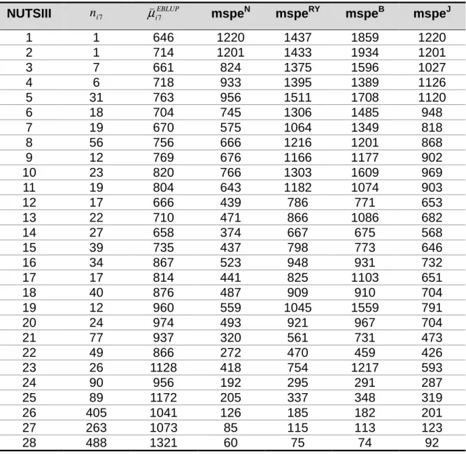
(6) small sample sizes, traditional direct estimators are either not feasible or provide unacceptably large variation coefficients. Therefore, indirect estimators are needed in order to “borrow information” from related small areas and time periods through linking models, using recent census and current administrative data. In this application, we use the temporal EBLUP assisted by the Rao-Yu model. As the Portuguese Statistical Office also conducted the Prices of Bank Evaluation in the Habitation Survey (PBEHS), we decided to use the bank evaluation of the habitations as auxiliary variable. Both the target variable and the auxiliary variable are measured in euros by square meter. Furthermore, the data are available on a quarter basis from seven time points, t=1, …, 7. Table 1. Small areas, sample sizes, EBLUP estimates of mean price of the habitation transaction in the 7th wave and their naïve, analytical, bootstrap and jackknife MSPE estimates ( ni 7 µ i7EBLUP NUTSIII mspeN mspeRY mspeB mspeJ 1 2 3 4 5 6 7 8 9 10 11 12 13 14 15 16 17 18 19 20 21 22 23 24 25 26 27 28. 1 1 7 6 31 18 19 56 12 23 19 17 22 27 39 34 17 40 12 24 77 49 26 90 89 405 263 488. 646 714 661 718 763 704 670 756 769 820 804 666 710 658 735 867 814 876 960 974 937 866 1128 956 1172 1041 1073 1321. 1220 1201 824 933 956 745 575 666 676 766 643 439 471 374 437 523 441 487 559 493 320 272 418 192 205 126 85 60. 1437 1433 1375 1395 1511 1306 1064 1216 1166 1303 1182 786 866 667 798 948 825 909 1045 921 561 470 754 295 337 185 115 75. 1859 1934 1596 1389 1708 1485 1349 1201 1177 1609 1074 771 1086 675 773 931 1103 910 1559 967 731 459 1217 291 348 182 113 74. 1220 1201 1027 1126 1120 948 818 868 902 969 903 653 682 568 646 732 651 704 791 704 473 426 593 287 319 201 123 92. 6.

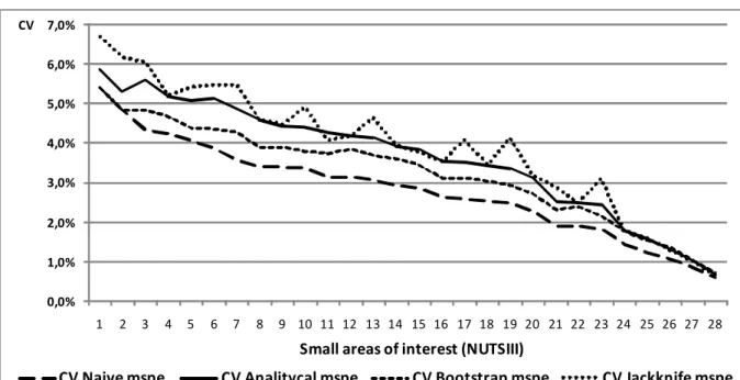
(7) In this application, the target parameter of interest is the mean price of the habitation transaction per square meter by NUTSIII level (28 small areas, i=1, ..., 28). Estimatives of this parameter are given by the temporal EBLUP after fitting the RaoYu model to PHTS and PBEHS data. Afterwards, we analyse different measures of uncertainty of this EBLUP: the naive (6), the analytical (7), the bootstrap (8) and the linearized weighted jackknife (9) MSPE estimators. Table 1 shows by small areas (NUTSIII), the sample sizes in the 7th wave ( ni 7 ), ( EBLUP estimates of mean price of the habitation transaction in the same wave ( µ i 7 ) and the corresponding uncertainty measures over small areas. The coefficients of variation (vc) of temporal EBLUP estimates of mean price of the habitation transaction are plotted in figure 1. The coefficient of variation is defined as ( ( mspeit θ it (ψˆ ) θ it (ψˆ ) . From this figure we can observe a similar behavior for all. [. ]. uncertainty measures of the temporal EBLUP. The Jackknife estimator is the one exhibiting a more specific pattern as it does not show a totally monotonic decrease of the variation coefficients along with areas 1 to 28. We can also see that the bootstrap-based coefficients of variation are lower than the analytical and jackknifebased ones. The naïve estimator is the one producing the smaller variation coefficients, as was expected according to the theory, since this estimator is known to underestimate the true MSPE. The results confirm a good precision of the EBLUP estimates even when the sample sizes are very small, since all coefficients of variation are below 7%. Obviously the precision of the EBLUP estimates for small areas 24-28 are also very good, since they have large sample sizes. Figure 1. Coefficients of variation for the EBLUP estimates of mean price of the habitation transaction in the 7th wave CV 7,0% 6,0% 5,0% 4,0% 3,0% 2,0% 1,0% 0,0% 1. 2. 3. 4. 5. 6. 7. 8. 9 10 11 12 13 14 15 16 17 18 19 20 21 22 23 24 25 26 27 28. Small areas of interest (NUTSIII) CV Naive mspe. CV Analitycal mspe. CV Bootstrap mspe. CV Jackknife mspe. 7.

(8) 5. Concluding remarks Statistical offices are currently required to provide small area estimates, but as sample surveys are usually designed to produce estimates for large planned domains, model-based methods can be used to provide reliable indirect estimators at small area level. In this paper, a temporal EBLUP estimator was used to provide estimates of mean price of the habitation transaction at NUTSIII level. The coefficients of variation of these estimates were assessed by the naive, analytical, bootstrap and weighted jackknife MSPE estimators. The results reveal that all MSPE estimators present similar behavior over the small areas, although the naive MSPE estimator tends to underestimate the MSE, as was said previously. Results confirm that the use of the temporal EBLUP offers good precision when estimating the price of habitation transaction even for domains with very small sample size. Furthermore, the results suggest that the linearized weighted jackknife MSPE estimator could be the best resampling-based estimator to assess the uncertainty of the mean price of the habitation transaction EBLUP estimates. This is due to its similarity to the analytical MSPE estimator and its ability to produce results less smooth than the ones achieved by the other estimators.. Acknowledgements The authors acknowledge the Portuguese Statistical Office for the availability of the data used in the research. The first author’s research was supported in part by the Portuguese Foundation for Science and Technology (fellowship SFRH/BD/36764/2007).. References Butar, F.B., and Lahiri, P. (2003). On measures of uncertainty of empirical Bayes small area estimators. Journal of Statistical Planning and Inference, 112, 63-76. Das, K., Jiang, J., and Rao, J.N.K. (2004), “Mean squared error of empirical predictor”, The Annals of Statistics, 32, pp. 818-840. Datta, G.S., and Lahiri, P. (2000), “A unified measure of uncertainty of estimated best linear unbiased predictors in small area estimation problems”, Statistica Sinica, 10, pp. 613-627. Fay, R.E., and Herriot, R.A. (1979), “Estimates of income for small places: An 8.

(9) application of James-Stein procedures to census data”, Journal of the American Statistical Association, 74, pp. 269-277. Henderson, C.R. (1953), “Estimation of variance and covariance components”, Biometrics, 9, pp. 226-252. Jiang, J., and Lahiri, P. (2006), “Mixed Model Prediction and Small Area Estimation”, Test, 15(1), pp. 1-96. Jiang, J., Lahiri, P. and Wan, S.-M. (2002), “A unified jackknife theory for empirical best prediction with M-estimation”, The Annals of Statistics, 30, pp. 1782-1810. Pereira, L.N., and Coelho, P.S. (2009), “Assessing different uncertainty measures of EBLUP: a resampling-based approach”, Journal of Statistical Computation and Simulation, forthcoming. Prasad, N.G.N., and Rao, J.N.K. (1999), “On robust small area estimation using a simple random effects model”, Survey Methodology, 25(1), pp. 67-72. Rao, J.N.K. (2003), Small area estimation, New Jersey: John Wiley & Sons. Rao, J.N.K., and Yu, M. (1994), “Small-area estimation by combining time-series and cross-sectional data”, The Canadian Journal of Statistics, 22(4), pp. 511-528.. 9.

(10)