THE IMPACT OF JELLYFISH ON THE
ESTUARINE ECOSYSTEMS: THE GUADIANA
STUDY CASE
Teja Petra Muha
Dissertation of Master thesis by
Erasmus Mundus Master of Science on Ecohydrology
Advisors
Prof. Dr. Maria Alexandra Anica Teodósio Chícharo
Dr. Radhouan Ben-Hamadou
Prof. Dr. Luis Chicharo
2 Copyright Teja Petra Muha
A Universidade do Algarve tem o direito, perpétuo e sem limites geográficos, de arquivar e publicitar este trabalho através de exemplares impressos reproduzidos em papel ou de forma digital, ou por qualquer outro meio conhecido ou que venha a ser inventado, de o divulgar através de repositories científicos e de admitir a sua cópia e distribuição com objetivos educacionais ou de investigação, não comerciais, desde que seja dado crédito ao autor e editor.
Declaração de autoria de Trabalho
Declaro ser a autora deste trabalho, que é original e inédito. Autores e trabalhos consultados estão devidamente citados no texto e constam da listagem de refências incluida.
3 Author: Teja Petra Muha¹
Thesis supervised by: Prof. Dr. Maria Alexandra Teodósio Chicharo², Prof. Dr. Luis
Chicharo¹, Dr. Radhouan Ben- Hamadou²
Affiliation address: 1- Faculdade de Ciências e Tecnologia, Universidade do Algarve,
8005-139 Faro, Portugal, 2- CCMAR Universidade do Algarve, 8005-139 Faro, Portugal
Corresponding author- E-mail address: [email protected] Scientific area: Marine Ecology/ Coastal Ecohydrology
Key words: newly introduced species, Blackforida virginica, modeling, food web
dynamics, flow changes, zooplankton, ichthyoplankton
Palavras-chave: espécies invasoras, Blackforida virginica, modelação, dinâmica da teia
trofica, alterações de caudal, zooplâncton, ictioplâncton
Date: 13th of December 2013
Title of dissertation: The impact of jellyfish on the estuarine ecosystems: the Guadiana
4
To Lana,
my newly born sweetheart,
5 Abstract
The presence of newly introduced species of jellyfish in the estuarine systems can result in diverse disruptions at different levels of the food web affecting native competitor species, predators and prey. Newly introduced species of jellyfish can poses a threat to this system by affecting the well- established food web dynamics. There was a noticeable increase in jellyfish presence in years after the Alqueva dam in relation to the species
Aurelia aurita, Blackfordia virginica, Maeotias marginata and Catostylus tagi. B. virginica has become the most widely spread species within the Guadiana Estuary. Its
presence might be an important factor influencing the pelagic ecosystem in Guadiana by predation effect and competition with other predators. As zooplankton presents a main food source for zooplanktivorous fish and fish larvae the jellyfish species may be able to over compete the native fish population or decrease the food supply to insufficient level. This could directly result in decrease of zooplankton abundance correlated to an increase of phytoplankton and consequently in eutrophication. Presumably there is a potential for jellyfish species annual growth and establishment. This work presents a food web model located in the Guadiana Estuary situated between South of Spain and Portugal where the impact of jellyfish B. virginica was evaluated in a model based on the variation of biomass of each state variable (mgC m-3). B. virginica has been present in the estuary since 2002 with the highest abundance of 31.2 ind. m-3 measured in 2008. The Guadiana Estuary had experience significant changes related to fresh water availability as Alqueva dam was built in 2002. What impact does water discharge and pattern of precipitation rate related to NAO has on present ecosystem has been evaluated through the nutrient and seston concentration in the model. Extential sampling data from year 1997 up to 2012 was conducted in Guadiana Estuary which data were used through the process of
statistical analysis for the model functioning. Guadiana Estuary is divided into three sub-areas: upper with stations Alcotium and Gueirros do Rio; middle with sampling at Almada de Ouro and Foz de Odeleite; and lower estuary where samples were taken at Esteiro Carrasqueira, Barra, River Plume (Pluma) and Praia de St. Antonio station.
6
Presence of B. virginica normally takes place in brackish zone where ETM zone is present which is characterized by mixed salinity. We have developed a seasonal food-web model based on the annual presence of jellyfish B. virginica, which is from beginning of June to the end of August. We have used 6 groups of marine organisms represented as state variables in the model. Groups of phytoplankton, zooplankton, ichthyoplankton (fish eggs and fish larvae separated), B. virginica, juvenile European anchovy (Engraulis encrasicolus) and their biomass, distribution, and diet were used from survey data. Food web model was created within the most important groups in the ecosystem and presented in the conceptual diagram. For our theoretical network model we have worked on a predator- prey relation expressed with the Michaelis- Menten exponential response. Through different sensitivity tests we have shown the potential impact of jellyfish species on the present food web through different scenarios. Statistical analysis based on average abundance rate of B. virginica and zooplankton compared to abiotic conditions was done for an easier clarification and comparison with the results from the model. The results obtained by the model developed in this thesis are in conformity with field measurements to what it concerns biomass values of each
individual group in the model. The model shows a significant impact of B. virginica over all groups of species presented in the model. Nutrient and seston concentration appears to be the most influential trigger for the majority of the food web dynamics. Sensitivity analysis has proven that the phytoplankton, zooplankton and juvenile anchovy are the most sensitive organisms in the whole food web influenced by nutrient availability and water discharge. B. virginica, fish eggs and fish larvae biomass has proven to vary upon these conditions tested in different runs though they are not affected directly. There is significantly high jellyfish biomass increase in case of high nutrient concentrations. In similar situation if B. virginica is not present there is a high rise in ichthyoplankton biomass, juvenile anchovy and zooplankton. Situation with low water discharge and high nutrient amount appears to be the most devastating for the estuarine ecosystem. In
situation with low nutrient conditions the phytoplankton, fish eggs, fish larvae and B.
7
biomass decreases. Trend of this groups tend to change in different nutrient conditions. Significant changes in biomass content are noticed between all groups. Compared to low nutrient concentration simulations in high nutrient concentration present that all state variables have an initial increase and only due to the predatory effect the decrease of certain groups occur. Detritus production trend follows up the movement of biomass increase and decrease. There is a strong correlation of B. virginica increase due to
predational effect over zooplankton which levels seem to be detrimental for the fish eggs. Fish larvae group appears to be the most resistant group for the B. virginica pressures on the ecosystem. By the results in the model we can see that the NAO index can reflect a pattern of each individual biomass group in the food web as it is partially responsible for the nutrient concentration in the estuary. The most impacted group by B. virginica is zooplankton which controls phytoplankton growth from top down. These relation causes bottom up control as zooplankton biomass influences the ichthyoplankton and juvenile anchovy biomass. In case of high winter water discharge the detritus production is higher and the turbidity at the mouth of the estuary attracts higher amount of adult’s fish to spawn. Higher fish eggs biomass causes higher and faster growth of B. virginica which is able to consume higher amount of zooplankton and with that controls the decrease in juvenile anchovy population and fish larvae survival rate. Possible presented scenario is over- predation of zooplankton which can lead to phytoplankton bloom.
Resumo
A presença de espécies de medusas recentemente introduzidas nos sistemas estuarinos pode resultar em diversas rupturas nos diferentes níveis da teia alimentar afetando espécies nativas competidoras, predadores e presas. Espécies recentemente introduzidas de representam uma ameaça para este sistema, afetando a dinâmica da rede trofica. Houve um registo de frequência medusasapós a construção da barragem do Alqueva, de especeis de organismos gelatinosos, como e Aurelia aurita, Blackfordia virginica,
8
espécie mais representada dentro do Guadiana Estuário. A aua presença pode ser um fator importante que influencia o ecossistema pelágico no Guadiana através do potencial de predação e competição com outros predadores. Como zooplâncton apresenta a principal fonte alimentar para larvas de peixe e peixe zooplanktivorous, estas espécies podem ser capazes de competir com a população de peixes nativos ou diminuir a oferta de recursos pesqueirospara o nível insuficiente. Outra consequencia seria a redução de zooplâncton e um consequente um aumento de fitoplâncton e, provavel, na eutrofização. Este trabalho apresenta um modelo de teia alimentar para o Estuário do Guadiana situado entre o Sul de Espanha e Portugal, onde o impacto da medusa B. virginica foi avaliada com base na variação da biomassa de cada variável de estado (mgC m-3 ). B. virginica esteve presente no estuário desde 2002, com a maior abundância de 31. 2 ind. m-3 medido em 2008. O Guadiana Estuário sofreu mudanças significativas em relação à disponibilidade de água doce em aprticular após a construção da barragem doAlqueva em 2002. Qual o impacto que descarga de água e padrão de taxa de precipitação relacionada com NAO tem no presente ecossistema tem sido avaliada através da concentração de nutrientes e seston no modelo. Dados de amostragem desenvolvidas de 1997 até 2012, no Estuário do Guadiana foram utilizados durante o processo de análise estatística sobre o
funcionamento do modelo de. Guadiana Estuário está dividido em três sub-áreas : superior, com estações Alcotium e Guerreiros do Rio ; medio com estaçoes em Almada de Ouro e Foz de Odeleite , e inferior com estações no Esteiro Carrasqueira , Barra , Pluma e Praia de St. Antonio. A presença de B. virginica normalmente ocorre na zona salobra zona onde a ETM estiver presente, e caracteriza-s por uma zona de mistura de salinidade. Desenvolveu-ses um modelo sazonal –de teia trofica com base na presença anual de B. virginica , entre o início de junho até final de agosto. Usaram-se 6 grupos de organismos marinhos representados como variáveis de estado do modelo:fitoplâncton, zooplâncton, ictioplâncton (ovos e larvas de peixes peixe separados), B. virginica, juvenil de anchova europeia (Engraulis encrasicolus) e sua biomassa, a distribuição e dieta foram utilizados a partir de dados de pesquisa. O Modelo da teia trofica foi criado dentro dos grupos mais importantes no ecossistema e apresentados no diagrama conceitual. Para
9
o nosso modelo de rede teórica trabalhou-se numa relação predador-presa expressa com a resposta exponencial Michaelis -Menten. Através de diferentes testes de sensibilidade que têm demonstrado o impacto potencial das espécies de medusa na presente teia alimentar através de diferentes cenários. A análise estatística das taxas abundância média de B. virginica e zooplâncton e em comparação com as condições abióticas foi feito para uma validaçãoe comparação com os resultados do modelo.Os resultados obtidos pelo modelo desenvolvido nesta tese estão em conformidade com as medições de campo para o que diz respeito a valores de biomassa de cada grupo individual no modelo. O modelo mostra um impacto significativo de B. virginica sobre todos os grupos de espécies incluidas na analise. A concentração de nutrientes e séston parece despoletar a dinâmica da teia alimentar. A análise de sensibilidade mostrou que o fitoplâncton , zooplâncton e anchova juvenil são os organismos mais sensíveis em toda a teia alimentar influenciada pela disponibilidade de nutrientes e descarga de água doce. B. virginica, ovos de peixe e biomassa de larvas de peixes provou variar de acordo com estas condições testadas em testes diferentes, embora eles não sejam afetados diretamente. Não é significativamente elevado aumento da biomassa medusas em caso de altas concentrações de nutrientes. Em situação semelhante se a B. virginica não está presente há um elevado aumento na
biomassa ictioplâncton, anchova juvenil e zooplâncton. Em situação de baixa descarga de água docee elevada quantidade de nutrientes parece ser a mais devastadora para o
ecossistema estuarino. Em situação com baixas condições de nutrientes, de fitoplâncton, ovos e larvas de peixes, a biomassa B. virginica aumenta ao longo verão, mas o
zooplâncton e a biomassa juvenil de anchova diminuiu. A importância destes grupos tende a mudar em diferentes condições nutricionais. As mudanças significativas no teor de biomassa são notorios entre todos os grupos. A comparação com as simulações de concentração de nutrientes baixos a alta concentração de nutrientes presentes provoca em todas as variáveis de estado um aumento inicial e só devido ao efeito predatório a
diminuição de certos grupos ocorre. A tendência de produção de detritos acompanha o movimento de aumento da biomassa e sua redução. Há uma forte correlação entre aumento B. virginica devido ao efeito predatório sobre o zooplâncton que os níveis
10
parecem ser prejudicial para os ovos de peixe. O grupo larvas de peixes parece ser o grupo mais resistente para as pressões B. virginica sobre o ecossistema. Pelos resultados do modelo, podemos ver que o índice NAO pode indicar um padrão da biomassa
individual na teia trofica, uma vez que é parcialmente responsável pela concentração de nutrientes no estuário. O grupo mais afetado por B. virginica é zooplâncton que controla o crescimento do fitoplâncton , de cima para baixo. Esta relação causa um controle pela basepois a biomassa de zooplâncton influencia o ictioplâncton e biomassa juvenil anchova. Em caso de de alta descarga de água doce no inverno a produção de detritos é maior e a turbidez na foz do estuário atrai maior quantidade de adultos para desovar e para a pesca. Maior biomassa de ovos de peixe provoca um crescimento maior e mais rápido de B. virginica que é capaz de consumir maior quantidade de zooplâncton e com que controla o decréscimo na população de anchova juvenil e taxa de sobrevivência de larvas de peixes. Como conclusão pode-se referir que os resultados obtidos com o modelo desenvolvido nesta tese estão em conformidade com as medições realizadas in situ no que se refere aos valores de biomassa de cada grupo individual. Para além disso é um dos poucos estudos existentes a nível da etia trófica, onde as medusas são incluidas como grupo individual.
11 Table of Contents Abstract ... 5 Resumo ... 7 Context of tables: ... 15 Introduction ... 16 Methodology ... 24 Study area ... 24 Model run ... 26 Results ... 41
1. Run 1, after dam, Q (summer discharge)=7.5 m3 s-1, BN =0.004 µmol m-3, SSC=0.00003 mg m-3 ... 46
2. Run 2, after dam, Q (summer discharge)= 2.75 m3 s-1, BN =0.0015 µmol m-3, SSC=0.00002 mg m-3 ... 54
3. Run 3 has some conditions as run 2 (BN =0.0015 µmol m-3, SSC=0.00002 mg m-3- low nutrient conditions) but there is an increase in initial levels of B. virginica from 0.003 to 0.03 mgC m-3. ... 57
4. Run 4 have some conditions as run 2 (BN =0.0015 µmol m-3, SSC=0.00002 mg m-3- low nutrient conditions) with no presence of Blackorida virginica. ... 58
5. Run 5, before dam, Q (summer discharge) 38 m3 s-1, BN =0.6 µmol m-3, SSC=0.32 mg m-3 ... 59
6. Run 6, before dam, Q (summer discharge) 15 m3/s, BN =0.009 µmol m-3, SSC=0.0145 mg m-3 ... 64
7. Run 7 have some conditions as run 6 (BN =0.009 µmol m-3, SSC=0.0145 mg m-3) but there is an increase in initial levels of B. virginica from 0.003 to 0.03 mgC m-3. ... 66
12
8. Run 8 have some conditions as run 4 (BN =0.009 µmol m-3, SSC=0.0145 mg
m-3) only with B. virginica biomass=0. ... 67
Discussion ... 70
Conclusion ... 86
Acknowledgments... 89
References ... 90
Annex: ... 105
I. Conversion rates for parameters used in the model. ... 105
Table of figures: Figure 1-Upper part- juvenile pelagic Blackfordia virginica; lower part-polyps of some species, hydroid stage; http://invasions.si.edu/nemesis/browseDB/SpeciesSummary.jsp?TSN=49780. ... 18
Figure 2- Guadiana river and estuary on the border between Spain and Portugal including sampling points (Morais et al., 2009). ... 26
Figure 3- Conceptual diagram including all state variables used in the model, where narrow arrows represent predation, dotted arrows present dead organic material (detritus) contributing to detritus box. ... 31
Figure 4- Average of B. virginica (ind. m-3) densities through presented years at each individual sampling station. ... 42
Figure 5- Mean abundance of B. virginica (individuals m-3) compared to mean annual water discharge in winter Q (m3 s-1) from year 1997 up to 2011. ... 43
Figure 6- Mean abundance of B. virginica (individuals m-3) compared to mean NAO (North Atlantic Oscillation) index from year 1997 up to 2011. ... 44
Figure 7- Mean abundance of B. virginica (individuals m-3) compared to mean zooplankton abundance (individuals m-3) between years 1997 up to 2011. ... 45
13
Figure 9- Biomass variation of organic carbon of each individual group (mgC m-3) in the
Guadiana Estuary over period of 90 days under conditions of run 1. ... 48 Figure 10- Biomass variation of phytoplankton (mgC m-3), zooplankton, fish larvae, B.
virginica, fish eggs and juvenile anchovy (mgC m-3) through time series of 90 days in
summer conditions and nutrients availability by run 1. ... 49 Figure 11- Biomass variation of fish eggs (mgC m-3) through time series of 90 days in
summer conditions and nutrients availability by run 1. ... 50 Figure 12- Biomass variation of juvenile anchovy Engraulis encrasiocolus (mgC m-3)
through time series of 90 days in summer conditions and nutrients availability by run 1. ... 51 Figure 13- Detritus production as organic carbon content of phytoplankton (mgC m-3),
zooplankton, ichthyoplankton (fish larvae and fish eggs), B. virginica and juvenile anchovy (mgC m-3) through time series of 90 days in summer conditions and nutrients
availability by run 1. ... 52 Figure 14- Total detritus production (mgC m-3) jointly together by all state variables in
through summer time by nutrient availability in run 1. ... 53 Figure 15- Biomass variation of fish larvae and B. virginica (mgC m-3) through time
series of 90 days in summer conditions and nutrients availability by run 1. ... 53 Figure 16- Biomass variation of organic carbon of each individual group in the model
over period of 90 days under conditions of 2 run. ... 55 Figure 17- Biomass variation of phytoplankton (mgC m-3), zooplankton, fish larvae, B.
virginica, fish eggs and juvenile anchovy (mgC m-3) through time series of 90 days in
summer conditions and nutrients availability by run 2. ... 56 Figure 18- Biomass variation of fish larvae and B. virginica (mgC m-3) through time
series of 90 days in summer conditions and nutrients availability by run 2. ... 57 Figure 19- Biomass production of phytoplankton (mgC m-3), zooplankton, fish larvae, B.
virginica, fish eggs and juvenile anchovy (mgC m-3) through time series of 90 days in
14
Figure 20- Biomass production of phytoplankton (mgC m-3), zooplankton, fish larvae, B.
virginica (where biomass is 0), fish eggs and juvenile anchovy (mgC m-3) through time
series of 90 days in summer conditions and nutrients availability by run ... 59 Figure 21- Biomass variation of phtyoplankton (mgC m-3) through time series of 90 days
in summer conditions and nutrients availability by run 5. ... 61 Figure 22- Biomass variation of phytoplankton (mgC m-3), zooplankton, fish larvae, B.
virginica, fish eggs and juvenile anchovy (mgC m-3) through time series of 90 days in
summer conditions and nutrients availability by run 5. ... 62 Figure 23- Biomass variation of juvenile anchovy Engraulis encrasiocolus (mgC m-3)
through time series of 90 days in summer conditions and nutrients availability by run 5. ... 62 Figure 24- Total detritus production (mgC m-3) jointly together by all state variables in
through summer time by conditions in run 5. ... 63 Figure 25- Biomass variation of organic carbon (mgC m-3) of each individual group in
the model over period of 90 days under conditions of 5 run. ... 63 Figure 26- Biomass production of phytoplankton (mgC m-3), zooplankton, fish larvae, B.
virginica, fish eggs and juvenile anchovy (mgC m-3) through time series of 90 days in
summer conditions and nutrients availability by run 6. ... 65 Figure 27- Detritus production of phytoplankton (mgC m-3), zooplankton,
ichthyoplankton (fish larvae and fish eggs), B. virginica and juvenile anchovy (mgC m-3)
through time series of 90 days in summer conditions and nutrients availability by run 6. ... 66 Figure 28- Biomass variation of zooplankton, fish larvae, B. virginica and fish eggs (mgC
m-3) through time series of 90 days in summer conditions and nutrients availability by
run 6. ... 66 Figure 29- Biomass variation of zooplankton, fish larvae, B. virginica and fish eggs (mgC
m-3) through time series of 90 days in summer conditions and nutrients availability by
run 7. ... 67 Figure 30- Biomass production of phytoplankton (mgC m-3), zooplankton, fish larvae, B.
virginica, fish eggs and juvenile anchovy (mgC m-3) through time series of 90 days in
15
Figure 31- Biomass variation of fish larvae and B. virginica (mgC m-3) through time
series of 90 days in summer conditions and nutrients availability by run 8. ... 69 Figure 32- Biomass variation of juvenile anchovy (mgC m-3) through time series of 90
days in summer conditions and nutrients availability by run 8………69
Context of tables:
Table 1- Variables, coefficients for the model of Blackfordia virginica………..31 Table 2- Variables, for abiotic coefficients for the model of Blackfordia virginica…..36 Table 3- Differential equations for the model………...37
Table 4-Predation rates of B. virginica………..105
16 Introduction
The productive coastal areas of the oceans have been recognized as belonging to the most valuable ecosystems on Earth, from an ecological and socio-economic point of view (Costanza et al., 1997); yet, they are also among the most endangered due to a variety of direct and indirect anthropogenic disturbances such as pollution, marine and coastal construction, maritime transport, overfishing, invasive species, and climate change (Halpern et al., 2008, Nastav et al., 2013). The estuaries present a very powerful
connection between the inland waters and marine environment and with its specificness they are one of the most productive and fragile ecosystems (NOAA, 2012).
Anthropogenic modification of natural river pathways has been largely practiced in Spain (Alonso-Franco, 2003). Guadiana Estuary is no exception regarding increased
anthropogenic modifications. River regulation has normally a negative impact on the ecosystem. Dams constitute obstacles for longitudinal exchanges along fluvial systems and so result in “discontinuities” in the river continuum (Ward et al., 1995). Building of the Alqueva dam on Guadiana River, the largest dam structure in Europe, has definitely caused certain amount of modifications on the local natural environment, specifically on the downstream estuarine and adjacent coastal ecosystems. Its floodgates were closed on February 8th 2002. Since then, river flow regulation increased from 75% to 81% (Rocha
et al., 2002; Morais et al., 2009). Previous research have found increased modifications
within the ecosystem (Rocha et al., 2002, Chicharo et al., 2009b, Morais et al., 2009, Muha et al., 2012) after the closure of the dam. To what extent ecosystem is being
modified by variations in water discharge in the Guadiana Estuary Wolanski et al. (2006) presented in an ecohydrological model. With barriers on the river there is a consequential increase in water temperature which can provide potential new living places for the alien species that were limited before to the more equatorial waters. The newly introduced species particularly Cnidarians, jellyfishes are potential new colonizers of coastal environments with a great level of success at becoming a dominated organism in non-native ecosystem. The seasonal jellyfish bloom is common in many marine environments, but there is also great interannual variability (Purcell, 2005; Primo, 2012). In the
17
Guadiana jellyfish species are increasing annually as it comes to its biomass or species presence. The new introduction of the jellyfish species in the Guadiana is interestingly overlapping with the year of closure of the Alqueva dam. There was a noticeable increase in jellyfish presence in years after the Alqueva dam in relation to the species Aurelia
aurita, Blackfordia virginica, Maeotias marginata and Catostylus tagi. B. virginica has
become the most widely spread species within the Guadiana Estuary. Its presence might be an important factor influencing the pelagic ecosystem in Guadiana by predation effect and competition with other predators. Presumably there is a potential for jellyfish species annual growth and establishment.
Blackfordia virginica Majer (Fig. 1), 1910 is a well-known invasive medusa inhabiting
estuarine areas (Chicharo et al., 2009b). These hydromedusae, native to the Black Sea, are becoming a prominent feature of many estuarine communities (Mills, 2001). They have been established in estuarine areas around the entire world (Chicharo et al., 2009b). Yet, surprisingly little is known about their biological requirements, habitat use, and potential impacts where they have been introduced (Schroeter, 2008). Their appearance was previously investigated in Suisun Marsh in the upper San Francisco Estuary
(Schroeter, 2008, Mills et al., 1995, 2000), Napa and Petaluma Rivers (Wintzer et al., 2013) and Baltic Sea (Väinölä et al., 2013). They are identified as euryhaline species (Mills et al., 1995). B. virginica medusae are transparent, unpigmented, and delicate, with up to 80 very fine tentacles at maturity (Mills et al., 1995). B. virginica does not possess obvious light-sensing organs, but may still be responding to light-dark cues, as most gelatinous species are believed to have evolved some form of photoreception (Anderson, 1985, Wintzer et al., 2013).
18 Figure 1-Upper part- juvenile pelagic Blackfordia virginica; lower part-polyps of
some species, hydroid stage;
19
The B. virginica was observed in the Guadiana for the first time in July 2008, at the transitional zone of the estuary (brackish area) by (Chicharo et al, 2009b). High densities of medusae (> 100.100 ind. m-3) were collected in most samples from the Middle
estuary, with a maximum 3170.1 ind. 100 m-3 in (Posto Cinturão, geographic coordinates 37º15'30"N, 7º25'58"W). Specimens of both sexes were found, over a wide range of sizes (6-19 mm) and maturation stages and in such large numbers that would suggest local reproduction (Chicharo et al., 2009b). A minimum bloom initiation temperature of approximately 19 °C was assumed for release of medusae from polyps, when salinities are also suitable (Schroeter, 2008). Though there is an average biomass increase of B.
virginica in Guadiana no polyps have been found yet. New studies revealed that the
species was present already before in year 2002 and not in July 2008 as presented at the research (Chicharo et al., 2009b). There is no published information about the effects of
B. virginica on surrounding macrofauna or planktonic communities (Chicharo et al.,
2009b), as only the correlation with decreased abundance and composition of zooplankton can give us a clear image of their food resources.
The impacts of flow change are manifested across broad taxonomic groups including coastal and riverine plants, invertebrates and fish (Bunn et al., 2002). The changes in river inflow in our case lower water input in the coastal ecosystem can play a significant role on the reproduction of coastal species, limiting overall habitat availability (Bunn et
al., 2002), higher temperatures can cause stratification, lower input of nutrients, higher
retention time of organic matter, reduction in sediment input, longitudinal dispersal of migratory aquatic organisms (Bunn et al., 2002), declines in biodiversity and the alteration of natural food webs (Power et al. 1996) shifts in the water chemistry off coastal zones (Benstead et al., 1999), alterations in the distribution areas of zooplanktonic species (Kingsford et al., 1994; Chicharo et al., 2006a), invasions by alien species, effect on endemism (Bunn et al., 2002), changes in nutrient N:P:Si ratio can cause
eutrophication by the toxic algae blooms as for instance dinoflagellates as it was
20
success of exotic and introduced species in rivers is facilitated by the alteration of flow regimes (Bunn et al., 2002). As a consequence of intense shipping and opening of new transport routes, brackish habitats have been increasingly effected by nonindigenous species (NIS) (Paavola et al. 2005). To what extent river flow modifications affect species diversity in the Guadiana Ecosystem has been previously evaluated by Muha et al. (2012). To what extent river flow contributes to the effectiveness of NIS as jellyfish species are remains unclarified.
The amount of precipitation rate influencing on the amount of river discharge is a consequence of Northern Atlantic Oscillation (NAO index) that has a significant impact on the precipitation in Southern Europe. A low-pressure system over Iceland and a permanent high-pressure system over the Azores control the direction and strength of westerly winds into Europe. If the index is low (NAO-), westerly’s are suppressed and storms track southerly toward the Mediterranean Sea and increase the precipitation. When NAO is positive, there is less precipitation in Southern Europe. Since the NAO has the largest variability during the cold season, the loading pattern primarily captures characteristics of the cold season (NOAA, 2012). The correlation between NAO index and jellyfish abundance in Guadiana has been defined by Muha et al. (2012) though it would be interesting to know to what extent the precipitation rate influences on jellyfish dynamics on a wider scale.
Salinity gradient is a common feature of temperate estuaries having a pronounced spatial effect on the zooplankton composition and distribution (Azeiteiro et al., 1999). European brackish water seas (Baltic Sea, Black Sea and Sea of Azov, Caspian Sea) are subject to intense invasion of NIS (Paavola et al., 2005). In these seas, salinity is the most
important range limiting factor and native species seem to reach a minimum species richness at intermediate salinities (Paavola et al., 2005). A critical physical barrier is absent and gives these species a clear advantage in surviving ballast water voyages and initial introduction into a brackish water area (Paavola et al., 2005) which seems to be the way of B. virginica introduction to Guadiana Estuary.
21
Salinity and temperature gradient changes in the estuarine zone are consequences of water discharge variability and are responsible for the movement of estuarine turbidity maximum (ETM) zone. The newly introduced jellyfish species have settled in brackish zone where there is highly productive ETM zone and it’s theirs preferable habitat. In fact, in marine systems large aggregations of jellyfish are often found in areas of high turbidity and low light, where they have an advantage over visually feeding fishes (Eiane et al., 1999). A product of empty niches, suitable environmental conditions, and availability of proper vectors might be the most effective predictor for the invasibility of brackish water areas (Paavola et al., 2005). Lower densities of these species were noticed as well at lower or higher part of the estuary with different salinities ranging from 8- 28 PSU (Chicharo et al., 2009b) though in other research they have extended their presence from 3 to 35 PSU (Moore, 1987; Mills et al., 1995; Genzano et al., 2006). The brackish zone presents a focal area of presented model where predation impact by B. virginica is the most influential.
Blooms of jellyfish and ctenophores can attain enormous biomasses and cover extensive areas (Mills, 2001; Brodeur et al., 2002; Hay, 2006; Pitt et al., 2009). In many coastal and semi - enclosed areas (fjords, bays, and estuaries) gelatinous zooplankton are able to bloom and achieve enormous biomasses (tones per km 22) (Purcell, 2012, Brotz et al., 2012, Tinta et al., 2012). Jellyfish outbreaks can have many deleterious consequences, including losses in tourist revenue through beach closures and even the death of bathers (Purcel et al., 2007); power outages following the blockage of cooling intakes at coastal power plants (Purcel et al., 2007); blocking of alluvial sediment suction in diamond mining operations (Lynam et al., 2006); burst fishing nets and contaminated catches (Lynam et al., 2006); interference with acoustic fish assessments (Brierley et al., 2001); killing of farmed fish (Mills et al., 2001); reduction in commercial fish abundance through competition and predation (Lynam et al., 2006); and as probable intermediate vectors of various fish parasites (Hay et al., 2006, Richardson et al., 2009). Several studies had linked variations in jellyfish abundance with climate, particularly temperature
22
and salinity (Purcell, 2005, 2007) however the processes at play can differ by region (Primo, 2012). Jellyfish have a major impact (large footprint) on lower trophic levels but translate relatively little production to higher levels in the food web (small reach)
compared to forage fishes (Brodeur et al., 2007). Variety of B. virginica densities in the Guadiana Estuary can cause different responses to the well- established food web. Question remains what are the potential densities of the jellyfish that can cause deterioration or degradation of well- established food web in this estuarine area.
B. virginica feed primarily on pelagic invertebrates, although benthic/ epibenthic prey
and larval fishes were also found in the gut contents in a research done by (Wintzer et al., 2013). Wintzer et al. (2013) has defined B. virginica as being a non- selective
zooplankton predator. Stating that they are pelagic feeders, consuming both invertebrates and fish larvae. Copepod nauplii were by far most numerous prey in the guts, followed by cyclopoid copepods and mysids where all other prey items constituted less than 1% of the abundance in research done by Wintzer et al., (2013). Percent occurrence calculations for each item further support non-selective zooplankton feeding, with each prey item, except fish larvae, found in at least 50% of the sampling periods (Wintzer et al., 2013).
Otherwise the analysis of the gut contents of this alien medusa by Mills et al. (1995) indicated that they feed nearly exclusively on small planktonic crustaceans and no fish larvae or eggs were seen in any of the stomachs. Wintzer et al. (2013) could not find a correlation between prey number and bell diameter because of the wide variety of prey types, including both larger (i.e. fish larvae, mysids) and smaller (i.e. nauplii) items. With the help of detailed sampling data available at the time of B. virginica presence there is a potential to build up a food- web model based on their predation success and prey
availability.
Jellyfish biomass may decompose within the water column or on the benthos, depending on sinking rates and the depth of the water column as well as environmental conditions (Lebrato et al., 2011a, Tinta et al., 2012). Due to their high POC/PON and protein
23
content, nutrient recycling after decomposition of these blooms cause large
accumulations of inorganic nutrients to be released into the environment (Tinta et al., 2012), which can especially at stable no flux conditions further on cause eutrophication. The gelatinous biomass C/N is relatively low owing to a high nitrogen and low carbon content in the majority of the groups (C/N almost 20% lower than in other zooplankton groups, and overall it is between 10 and 20% lower than for phytoplankton and
phytodetritus/ marine snow/ faecal pellets) (Lebrato et al., 2011a).
Recognition and knowledge on what to expect in the future is on a high priority list nowadays. Defining possible scenarios with a help of models is crucial for the further management conclusions. Jellyfish species have not been previously used in a food-web model of Guadiana Estuary. What are the potential scenarios remains to be clarified. This study focuses on the impact of a newly introduced species of jellyfish B.virginica on the well- established food- web using modeling approach. The significance of the present study is correlated to a very well documented and researched history of Guadiana before the disturbance of jellyfish and as well a continuous research of the jellyfish presence. Extential sampling data from year 1997 up to 2012 was conducted in Guadiana Estuary which data will be used through the process of statistical analysis for the model
functioning. The abiotic conditions can significantly influence their dispersion which is evaluated through field sampling, statistical analysis and conclusively in a model. Our hypothesis is that climate-induced changes in ocean, biotic and abiotic conditions can cause variations in the amount of production that flows through the jellyfish population in the Guadiana Estuary. As B. virginica is newly introduced into the system we can study a potential reproductive and overall invasion success from its roots with the
implementation of ‘If case situations- sensitivity analysis’ scenarios to better understand or avoid a collapse of an existing food web. Through the model we will try to evaluate to what extent do jellyfish, namely B. virginica affect the survival and growth of
24
phytoplankton. We will define the amount of detritus produced by B. virginica under different scenarios in a model and individual detritus contribution of all individual groups of organisms. In the model we will evaluate how do fluctuations of organisms’ biomass change over the extended variety of nutrient concentration and which species or group of marine organism becomes predominant under certain conditions. Using a theoretical top-down and bottom-up model, we will examine variability in the transfer of energy
presented as biomass (mgC m-3) through alternate planktivore (jellyfish) pathways and use this to project possible changes in the food web within the estuary and coastal zone. With the use of bottom-up model we examine potential scenarios of varying energy flow through the jellyfish component and as well the influence of river flow dynamic on the entire food web. Well documented food web structures and alternate scenario strategies are being compared in the model. The mitigation measure is taken under consideration used through different water releases from the dam in order to measure the effects of such flow regulation to the downstream communities.
Methodology
Study area
The Guadiana Estuary constitutes the southern border between Portugal and Spain and its river basin is the fourth largest in the Iberian Peninsula, approximately 67 500 km2. The estuary is approximately 70 km long, encompassing a total area of 22 km2 and averaging 6.5 m in depth. It is a mesotidal estuary, with tidal amplitudes ranging from 1.3 to 3.5 m. The estuary is partially stratified when the average river flow (approx. 150 m3 s-1) and tidal prism (approx. 3×10⁷ m3) occur (Morais et al., 2009). The climate of the area is classified as semi-arid Mediterranean with the driest months in July and August when the river flow is the lowest. It is marked by the severe draughts and heavy floods. Climate variability imposes a similar trend to river flow; thus, the average river inflows are as follows: dry years, 8–63 m3 s-1; average years, 170–190 m3 s-1; humid years, 412–463
25
m3 s-1 (Bettencourt et al., 2003, Morais et al., 2009). Historical data of the freshwater flow measured at the hydrometric station of Pulo do Lobo (37°48´N, 7°38´W), located a few kilometers above the last point of tidal influence (Mértola) and from the most upper sampling station (Alcotium), refers values ranging between 6.07 m3 s-1 and 2491.70 m3 s-1. Mean river flow varies considerably depending on the season and on the year
(Ferreira et al., 2005). Strong interannual variation was also registered, being the average flow of the wettest year 436.4 m3 s-1 (in 1963/64), and 7.99 m3 s-1 in 1980/81 - the driest year recorded (Chicharo et al., 2009a). With the construction of the Alqueva Dam within this river basin in February 2002, which is one of the largest in Europe, those pulse events are smoothed (Machado et al., 2007).
Guadiana Estuary is divided into three sub-areas: upper with stations Alcotium and Gueirros do Rio; middle with sampling at Almada de Ouro and Foz de Odeleite; and lower estuary where samples were taken at Esteiro Carrasqueira, Barra, River Plume (Pluma) and Praia de St. Antonio station. This classification is commonly used to subdivide estuaries (Olausson et al., 1980, Chicharo et al., 2001a). Alcotium is considered as the uppermost station, situated in front of Alcotium (Portugal) at 38 km from the river mouth. The upper area is characterized by the freshwater dominance flow with salinity close to zero, where middle area is the salinity mixing zone (0.5- 25) and the lower part is characterized by the seawater intrusion dominance where salinity is above 25 (Chicharo et al., 2006a). The estuarine turbidity maximum zone before the dam filling was found between Foz de Odeleite and Almada de Ouro moving upstream to Guerrios do Rio after the closure. Presence of B. virginica normally takes place in brackish zone where ETM zone is present which is characterized by mixed salinity.
26 Figure 2- Guadiana river and estuary on the border between Spain and Portugal including sampling points (Morais et al., 2009).
Model run
The work was based on a theoretical non-dimensional model where we have evaluated biomass variations of each state variable under different scenarios (Figure 3). Presented possible scenarios are important factor for future management options. We can modify each individual state variable and relevant force in the model to see what could happen in certain case where models may combine several forces in continuous space and time. This gives as wider range and freedom compared to statistical models where only certain situation gives us a very narrow image of what is actually going on in the environment. Related literature to jellyfish presence and its impact on the environment is scarce and very much limited to statistics. Our trophic network model gives us new opportunity to evaluate the impact of jellyfish or other non-native species in hosting ecosystems which could guide decision makers towards mitigation or adaptation measures to limit the negative impact of these alien species.
27
We have developed a seasonal food-web model based on the annual occurrence of jellyfish B. virginica, which is from beginning of June to the end of August. We have used 6 functional groups of marine organisms gathered into state variables in the model. Groups of phytoplankton, zooplankton, ichthyoplankton (fish eggs and fish larvae separated), B. virginica, juvenile European anchovy (Engraulis encrasicolus) and their biomass, distribution, and diet were parameterized from survey data. In a model the energy flow of all state variables presented as biomass is simulated, where the competition between fish larvae and juvenile anchovy with B.virginica for the zooplankton is present as the only direct competitive process in a model. The
interrelations between state variables are presented in the conceptual diagram (Fig. 3). We have gathered information based on surveys done from year 1997 until 2011 to evaluate abiotic parameters and simulate them in the model before the Alqueva dam in 2002. Occurrence of B. virginica was detected from year 2002-2011. Abiotic parameters were consistently measured for chlorophyll a concentration, densities of all state variables (ind. m-3), Secchi disk, dissolved oxygen, temperature, salinity, water discharge (m3 s-1) (annual monthly & summer gathered), organic mater, solid SSC (mg L-1) (total solid material- Seston) and NAO index. Central to our method is the representation of mass-balance trophic flows between functional groups for basic parameterization as it was previously done in other models (i.e. ‘Ecopath models’). These interactions are run in the model as part of time series dynamic where different abiotic parameters and its values are being part of limitations. We have incorporated the light intensity as a forcing affecting phytoplankton growth and bottom-up control of the food web. Second bottom-up abiotic forcing is water discharge (m3 s-1) influencing on the amount of nutrients and total solid material in the estuary. The water discharge was a consequence of different precipitation rate which were a reflection of NAO index. The use of NAO index was indirect where only the consequence of an increased or decreased amount of average annual and summer water discharge has been used as a forcing in the model. It thus not directly reflects the value of an index but only the pattern related to water discharge. This water discharge
28
influences the amount of nutrients instantly. As for the fact that jellyfish contribute for large accumulations of inorganic nutrients we have incorporated detritus production into the food-web where the contribution of each individual state variable can be assessed.
For our theoretical network model we have worked on a predator- prey relation expressed with the Michaelis-Menten exponential (type II) response. One of the most popular mathematical model describing a predator-prey interaction is the following well-known Lotka-Volterra type predator-prey model with Michaelis-Menten (or Holling type II) functional response (Freedman, 1980, May, 1974):
( )
( ) ( ) eq.1 ( )
( ) eq.1
given that x(0) > 0 and y(0) > 0
where x and y stand for prey and predator density, respectively.
a,K, c,m,f,d are positive constants that stand for prey intrinsic growth rate, carrying
capacity, capturing rate, half saturation constant, maximal predator growth rate, predator death rate, respectively (Hsu et al., 2001).
This functional response is the intake or release rate of a predator as a function of food density. It is associated with the numerical response which is the reproduction rate of a consumer as a function of food density. Three types of Holling's cycles are I, II, and III, where we focused on the second one, present a functional response which is characterized by a decelerating intake rate, which follows from the assumption that the consumer is limited by its capacity to process food (Holling, 1959). The losses of state variables’s biomass were mortality, respiration and excretion. Migration pattern was not included in
29
the model for juvenile anchovy which needs for further discussion and development in future works. The energy flow within individual trophic groups follows a preposition:
Biomass (of state variables) = assimilation (or growth rate) respiration excretion -predation (mortality rate by -predation) – mortality (non- predatory mortality rate);
where excretion, respiration and mortality are not uniquely used for all state variables.
Because jellies have higher water content than other groups (Shenker, 1985, Ruzicka et al., 2012), we transferred all weights into carbon content to avoid overestimation of jellyfish biomass. For all the groups in a model the densities and concentrations were converted into the same units of milligrams of carbon per cubic meter (mgC m-3), except nitrogen as major part of nutrients in (µmol m-3). It is conventional to report biomass of jellyfish as dry or elemental (e.g., C or N) mass, yet most models are constructed using wet weight (i.e., tonnes km-2) (Pauly et al., 2009). Often the units reported were wet or dry weight or number of individuals per unit volume along where the conversions were necessary. For other correlation factors the units were modified into same form, rate (per day). We used species or taxa-specific conversions to carbon weight and other
conversions from variety of measures of ash free dry weight, dry or wet weight, jellyfish bell diameter or jellyfish length, growth rates, growth efficiencies, respiration rate, sloppy feeding, POC/ DOC excretion rates, assimilation efficiency, ingestion rates,
half-saturation constants for predator- prey relationship, predation rate, clearance and exudation rates. Preference was given to equations and measures from studies taken in the vicinity of the studies ecosystem (e.g. Ria Formosa coastal lagoon in Portugal) or similar environment and global zone. Physiological rate parameters, growth efficiency and others were obtained from other ecosystem models, literature of compared measures or calculated from local and other relevant data. All the variables, coefficients and
equations are found in tables 1, 2 and 3. Biomass values provided in table 1 are initial the lowest values of each state variable that was recorded in the same time of B. virginica presence that might be modified through different runs. These values might be modified later on through different runs and where the increase is stated separately at each run.
30
Conversions of individual parameter used in the model are found in annex I. In table 1 there are initial values of each state variables biomass. These values have been measured in the Guadiana and the lowest biomass presence in summer time was used for the initial biomass value in the model. Initial values of all state variables have been previously correlated to presence of B. virginica. Sampling data of state variables at the time when jellyfish was absent was not used, except in the model run when we have tested water discharge values and nutrient concentration in pre- dam situation. In table 3 there are all relevant differential equations each of them used in the model with 900 calculation loops through simulated 90 days.
Prey consumption rates by jellyfish can be estimated directly from gut contents (Purcell, 2003, Pauly et al., 2009), which in case of B.virginica was measured by Mills et al. (1995) and Wintzer (2013). Estimates of population production by jellyfish are rare and usually limited to rapid individual growth periods during the early phase of a cohort (Van der Veer et al., 1985, Olesen et al., 1994, Pauly et al., 2009). The diet of B. virginica was predisposed on the average feeding pattern by two studies (Wintzer et al., 2013, Mills et al., 1995) as measured predation rate and food type preferences. The diet breadth was broader by (Wintzer et al., 2013) than that found by Mills et al. (1995), in which 29 medusae from the Napa River fed exclusively on copepods, copepod nauplii, and
barnacle nauplii. Samples by Mills et al. (1995) were collected on a single day late in the bloom season, which may explain the discrepancy. An average predation rate of both reviewed journals was used as an average prey type for further on calculation of prey biomass.
In order to calibrate our model statistical analysis were done using SPSS programme. Graphical representation of B. virginica density (ind. m-3) compared with abiotic
components are discussed further on. Statistical analysis based on average abundance rate of B. virginica and zooplankton compared to abiotic conditions was done for an easier clarification and comparison with the results from the model. Statistical representations
31
of results are an initial step towards the reliability of the model where both conditions are compared.
Figure 3- Conceptual diagram including all state variables used in the model, where narrow arrows represent predation, dotted arrows present dead organic material (detritus) contributing to detritus box.
Table 1- Variables, coefficients for the model of Blackfordia virginica
Coefficients Definition Units Values (in.= initial)
References
Biotic, state variables
32 BN Initial concentration of nutrients (Nitrate) µmol m-3 (from 0.0015 up to 0.6 tested in a model) On site observations satNP Half-saturation constant* for phytoplankton with nitrate
µmol N_1 0.6 Chicharo et al., 2006a (Diatoms for nutrients) SSC Seston- organic material mgC m-3 From 0.00002 up to 0.32 On site observations kBN Maximum uptake rate for diatoms
per day 0.8 Chicharo et al., 2006a
AssNP Assimimation
rate of nitrogen
per day 0.95 Calibration
BP Initial biomass for phytoplankton mgC m-3 1.34 On site observations excp Exudation constant for phytoplankton
per day 0.013 Nagata, 2000
RespP Respiration
constant for phytoplankton
per day 0.01 Kromkamp et al., 1995
kp1 Growth rate of phytoplankton
per day 0.9 Paerl et al., 2006
33
1976
morp Phytoplankton
mortality not due to predation
per day 0.03 Scavia et al., 1976 satPZ Half-saturation constant* for zooplankton in phytoplankton mgC m-3 0.85 Jorgensen,1976 BZ Initial biomass for zooplankton mgC m-3 0.56 On site observations
MorZ Mortality rate per day 0.005 Chen et al.,
1975
AssPZ Assimilation rate of phytoplankton by zoo (at 20ºC)
per day 0.75 Di Torro et al., 1971
PredZI Predation rate by ichthyoplankton
per day 0.074 Scavia, 1980
PredZB Predation rate by
B. virginica
per day 0.281 Wintzer 2013, Mills et al., 1995, modified satZI Half-saturation constant mgC m-3 0.0062 Fortier et al., 1996 satZB Half-saturation constant mgC m-3 0.18 Wintzer, 2013, modified BI Initial biomass for Fish larvae
mgC m-3 0.02 On site observations
34
efficiency of zooplankton
MorI Mortality rate
(for sardine postlarvae)
per day 0.012 Lenarz, 1972
RespI Respiration rate of fish larvae
per day 0.01 Kiorboe,1987
PredIB Predation rate of
B. virginica
per day 0.05 Wintzer, 2013
satIB Half-saturation constant fish larvae for B. virginica mgC m-3 120.28 Calibration BB Initial biomass for B. virginica mgC m-3 0.003 On site observations
RespB Respiration rate per day 0.014 Ishii et al., 2006
ExcB Excretion rate per day 0.0023 Calibration
AssZB Assimilation
efficiency of zooplankton by
B. virginica (for
other hydrozoa)
per day 0.68 Pitt et al., 2009
MorB Mortality rate of
B. virginica
per day 0.019 Calibration
AssIB Carbon
Assimilation rate of fish larvae by
B. virginica
per day 0.81 Pitt et al., 2009
35
biomass observations
keggs Growth rate of
fish eggs
per day 0.08 Kneib, 1993
Meggs Mortality rate
fish eggs
per day 0.007 Kneib, 1993
BBG Hatching rate success to fish larvae
per day 0.025 On site observations
satBeggsBB Half saturation concentration of fish eggs mgC m-3 0.0005 Calibration sateggs Half-saturation constant mgC m-3 1.35 Calibration
PredIEB Predation rate of
B. virginica on
fish eggs
per day 0.1 Mills et al., 1995, modified
AssIEB Assimilation
efficiency of B.
virginica for fish
eggs
per day 0.905 Pitt et al., 2009
BJ Initial biomass for Engraulis encrasicolus- juvenile anchovy mgC m-3 0.002 On site observations satZJ Half-saturation rate for anchovy
mgC m-3 0.4 Monteiro, 2001
AssZJ Assimilation
efficiency of zooplankton by
36
juvenile anchovy
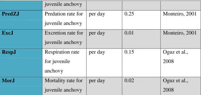
PredZJ Predation rate for juvenile anchovy
per day 0.25 Monteiro, 2001
ExcJ Excretion rate for juvenile anchovy
per day 0.01 Monteiro, 2001
RespJ Respiration rate for juvenile anchovy
per day 0.15 Oguz et al., 2008
MorJ Mortality rate for juvenile anchovy
per day 0.02 Oguz et al., 2008 * Half-saturation constant for the ith predator, which is the prey density at which the functional response of the predator is half maximal.
Table 2- Variables, for abiotic coefficients for the model of Blackfordia virginica
Abiotic variables, coefficients
lE Light intensity-Mean sunlight hours per day in Algarve (Jun-August)=10 hours Hour 10/ 14 sunlight/dar kness http://www.sagres.climatem ps.com/
Q Water discharge into the Estuary
m3 s-1 Variable
Model run works through a repeatedly set of equations based in a loop system with repeated frequency of 900 times calculations (Table 3). Each set of equation from the initial nutrient equation to final detritus production is correlated within the whole system.
37
Correlations between the equations in the model are based on the conceptual diagram. Light limitation equation is based on the amount of light availability through day time sinusoidal change for the summer time in the Algarve. It is directly influencing
phytoplankton growth. Nutrient concentration (nitrate) is represented correspondently to the amount of water discharge as part of the nutrient equation where initial concentration of nutrients (nitrate) (µmol m-3) is measured based on the average of summer monthly water discharge (m3 s-1) to corresponding concentration of nitrate (µmol m-3). Same evaluation is done for the seston which is representing the amount of solid organic material that enters the system. Detritus in the conceptual diagram represents the dead organisms, as well the equation for detritus is only the production of dead organic
material and the final amount is not recycled within the food web. We did incorporate the previously averaged amount of seston (solid organic material) as part of the first nutrient/ water discharge equation. It is though a simplified version of the amount available per cubic meter. The simplification is done from a reason that unknown amount of detritus is transferred out of the estuarine ecosystem. All the correlations are represented in the Table 3. This equation is correlated to phytoplankton Michaelis- Menten equation and is forcing phytoplankton growth by nutrient availability. Set of equations is written by the coefficients represented in Table 1. The coefficients tend to be unmodified unless specifically stated at each initial model run. Model runs were based on variations of sensitivity tests. For each sensitivity test there were changes done at the bottom of the food web as different amount of nutrients available for phytoplankton. For some
sensitivity tests there were different initial biomass of individual group used and nutrient amount was on its average after dam closure.
Table 3- Differential equations for the model Limitations in a model, forces:
38
( ) ( ( ) ) eq.2
kp=kp1*lE; where light limitation equation is directly related to phytoplankton growth rate
Nutrient (nitrate) concentration values corresponding to the average summer water discharge:
Before the dam:
38 m3 s-1=0.06 µmol m-3 27 m3 s-1=0.025 µmol m-3 15 m3 s-1=0.009 µmol m-3
After the dam:
7.5 m3 s-1=0.004 µmol m-3 4.4 m3 s-1=0.007 µmol m-3 3.75 m3 s-1=0.001 µmol m-3 2.75 m3 s-1=0.0015 µmol m-3
Seston- suspended solid organic material: Average of SSC (mg m-3) corresponds to average summer monthly water discharge (m3 s-1).
Before the dam:
38 m3 s-1=0.032 mg m-3 27 m3 s-1=0.02 mg m-3 15 m3 s-1=0.0145 mg m-3
After the dam:
39
9 m3 s-1=0.000672 mg m-3 7.5 m3 s-1=0.000023 mg m-3 2.7 m3 s-1=0.000018 mg m-3
Michaelis-Menten type 2 response: Nutrients:
( )
eq. 3
where ∂BN/∂t = nitrogen concentration variation through time series, kp= growth rate of phytoplankton based on light availability, ∂BP/∂t= phytoplankton biomass variation through time series, satNP= half-saturation constant for the ith predator, which is the prey density at which the functional response of the predator is half maximal (for
phytoplankton incorporation of nitrogen), SSC= Suspended solid organic material (mgC m-3). The rest of equations are calculated using same procedure, with different
coefficients and their description written in table 1.
Phytoplankton: ( ( )) (( ) ( )) ( ) eq.4 Zooplankton: (( ) ( )) (( ) ( )) (( ) ( )) (( ) ( ))
40 eq. 5 Ichthyoplankton: Fish larvae: (( ) ( )) ( ( )) (( ) ( )) ( ) eq.6 Fish eggs: ( ( )) (( ) ( )) eq. 7
Engraulis encrasicolus- juvenile european anchovy:
(( ) ( )) ( ) eq. 8 Blackforida virginica: (( ) ( )) (( ) ( )) (( ) ( )) ( ) eq. 9 Detritus:
41
( ) ( ) ( ) ( ) eq. 10
Each individual group:
( ) ; Detritus from Phytoplankton ( ; Detritus from Zooplankton ( ) ; Detritus from Ichthyoplankton
( ) ; Detritus from B. virginica ( ) ; Detritus from Juvenile anchovy
eq. 11
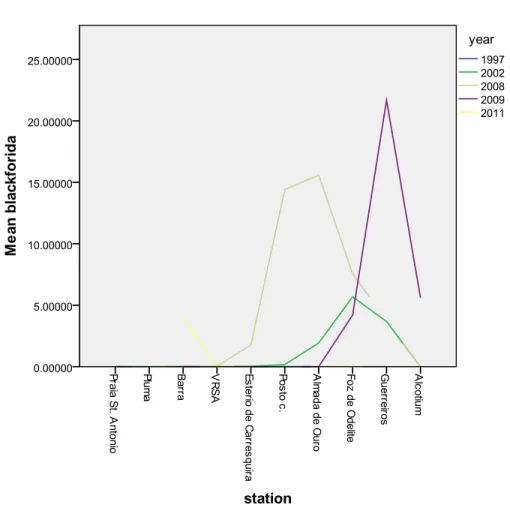
The average annual river water discharge after the Alqueva dam in years of B. virginica presence were 27.913 m3 s-1 (2002), 17.729 m3 s-1 (2008), 16.7 m3 s-1 (2009) and 191.235 m3 s-1 (2011). NAO index correspondingly to same years was 0.72 (2002), 2.1 (2008), -0.41 (2009) and -1.9 (2011). The average summer water discharge is
significantly lower in years after the Alqueva dam, with the exception of year 2011 due to high winter precipitation rate. B. virginica was not present before the dam closure but after 2002 there is a gradual increase of its biomass over years (Fig. 4). In the final sampling year of 2011 the density was low (below 5 ind. m-3) and it was found only at the mouth of the estuary. There is a strong inverse correlation between the B. virginica density and annual water discharge (Fig. 5) and strong positive relation to the NAO index with the abundance of jellyfish (Fig. 6). There is a positive correlation between the low density of zooplankton and high density of B. virginica where all zooplanktonic species are joint together (Fig. 7). Looking through species compositions comparing each individual station between each other there seems to be a correlation between lower species richness and higher evenness of zooplankton at the stations where there was also presence of the most abundant adult cnidarians B. virginica. These results are not
42
presented in statistical section but its percentages of species composition are used and recalculated in the calibration for the model. The strong correlation between water discharge, zooplankton and B. virginica density must not be overlooked where similarity of trends noticed between zooplankton density and water discharge are significant.
Figure 4- Average of B. virginica (ind. m-3) densities through presented years at each individual sampling station.
43 Figure 5- Mean abundance of B. virginica (individual’s m-3) compared to mean annual water discharge in winter Q (m3 s-1) from year 1997 up to 2011.
44 Figure 6- Mean abundance of B. virginica (individual’s m-3) compared to mean NAO (North Atlantic Oscillation) index from year 1997 up to 2011.
45 Figure 7- Mean abundance of B. virginica (individual’s m-3) compared to mean zooplankton abundance (individuals m-3) between years 1997 up to 2011.
Variation of phytoplankton biomass highly reflects variation of light availability within day and night cycle. Light intensity through the day and night cycle gradually changes from 0 to 1 during the 90 summer days cycle with accuracy of 2.4 h modification (Fig. 8). The frequency of 2.4 hours stays the same for each individual state variable recalculated through sets of equations. This defines certain sensitivity for each individual daily cycle of provided results in the model.
46 Figure 8- Light intensity variation through time series of 90 days.
1. Run 1, after dam, Q (summer discharge)=7.5 m3 s-1, BN =0.004 µmol m-3, SSC=0.00003 mg m-3
In this situation with low nutrient conditions the phytoplankton, fish eggs, fish larvae and
B. virginica biomass increases through summer but zooplankton and juvenile anchovy
biomass decreases (Fig. 9 and Fig. 10). Phytoplankton biomass stays low over the summer from 0.009 up to 0.9 mgC m-3 in first 70 days of model run which is related to efficient amount of predation pressure from zooplankton. After that the phytoplankton increases up to 250 mgC m-3. Zooplankton in the end of the summer time decreases after the initial rise up to 2 mgC m-3 to values of biomass that does not present significantly important contribution to the food web. The initial rise of zooplankton corresponds to the abundance of 4300 ind. m-3. This abundance corresponds to the measured densities in years with low water discharge especially the low biomass situation after first 30 days when the biomass is half of its maximum (Fig. 5 and Fig. 7). Biomass of fish eggs gradually increases up to 1 mgC m-3 (Fig. 11) where the constant contribution of fish eggs is included in the model through whole summer. Detritus contribution from all state
47
variables stays low over the summer from 0.06- 0.7 mgC m-3 and increases in the end of the summer up to 9 mgC m-3 which is strongly related to increased phytoplankton biomass (Fig. 14). The average detritus production over summer still remains higher for 10 or 100 fold increase than measured in years of low nutrient contribution. The largest contribution of detritus comes from phytoplankton (Fig. 13). The other groups contribute similar amounts around 0.005 mgC m-3. B. virginica biomass increase is correlated to decrease of zooplankton in first half of the summer, after that the biomass of fish eggs and fish larvae represent their main food source as zooplankton becomes depleted (Fig. 15). The highest achieved biomass is 0.45 mgC m-3 which corresponds to 750 ind. m-3 not yet measured abundance in Guadiana where the highest values (31.1 ind. m-3) measured in low water discharge conditions were in 2008 (Fig. 4).
After the initial increase the biomass of jellyfish drops and stays on the some level between 0.3-0.18 mgC m-3 which does present 10 fold increase to the measured rates in the Guadiana with similar nutrient conditions. Comparing the predational success between fish larvae group and jellyfish (Fig. 15), jellyfish tend to be much more successful as they their initial biomass is lower than fish larva but their predational impact is higher as their major increase compared to fish larvae is for 0.35 mgC m-3 higher in the middle of the summer. Juvenile anchovy Engraulis encrasiocolus biomass starts to decrease in the middle of summer due to depleted prey, zooplankton biomass (Fig. 12). The highest achieved value of 1.45 mgC m-3 drops to similar measured values in Guadiana. There is no significant difference of its biomass through the summer. The migration of juvenile anchovy in the end of the summer out of the estuary is not included in the model. In that case the zooplankton biomass would be higher in the second half of the summer.
48 Figure 9- Biomass variation of organic carbon of each individual group (mgC m-3) in the Guadiana Estuary over period of 90 days under conditions of run 1.
49 Figure 10- Biomass variation of phytoplankton (mgC m-3), zooplankton, fish larvae,
B. virginica, fish eggs and juvenile anchovy (mgC m-3) through time series of 90
50 Figure 11- Biomass variation of fish eggs (mgC m-3) through time series of 90 days in summer conditions and nutrients availability by run 1.
51 Figure 12- Biomass variation of juvenile anchovy Engraulis encrasiocolus (mgC m-3) through time series of 90 days in summer conditions and nutrients availability by run 1.