Comparison of sonographic techniques for the assessment of biceps femoris long head architecture

(1)

UNIVERSIDADE DE LISBOA

FACULDADE DE MOTRICIDADE HUMANA

UNIVERSIDADE DE LISBOA

FACULDADE DE MOTRICIDADE HUMANA

Comparison of sonographic techniques for the

assessment of biceps femoris long head architecture

Dissertação elaborada com vista à obtenção

do Grau de Mestre em Treino de Alto Rendimento

Orientador:

Doutor Sandro Remo Martins Neves Ramos Freitas

Júri:

Doutor Anthony John Blazevich

Doutora Filipa Oliveira da Silva João

Ricardo Jorge Lemos Pimenta

(2)

iii

AGRADECIMENTOS

Em primeiro lugar, gostaria de salientar que desde jovem a obtenção deste mestrado passava pelos meus planos. Na infância comecei a minha ligação com o desporto, nomeadamente o futebol, com o passar dos anos comecei a querer entender como poderia melhorar o meu rendimento. Nessa altura, as pesquisas eram bem diferentes das de agora, mas o objetivo foi sempre o mesmo, tornar-me um profissional de excelência no ramo do treino de alto rendimento. Desta forma, para estar no caminho da excelência só faria sentido entrar para este mestrado.

A concretização deste feito, deve-se essencialmente a todas as condições que os meus pais me conseguiram proporcionar até estar aqui presente. Assim sendo, o primeiro agradecimento é dirigido em conjunto, aos meus pais. Agradecer à minha mãe por todo o apoio demonstrado ao longo desta caminhada, estando sempre do meu lado nas decisões que tomei. Agradecer ao meu pai, por todos os valores que me transmitiu e incutiu desde criança. De realçar, valores que foram importantes para esta jornada, como a resiliência, ambição e postura de trabalhador. Estas duas pessoas são os pilares da minha vida e que se este grau de mestre é uma realidade, deve-se fundamentalmente a vocês. Obrigado!

Gostaria também de agradecer, ao professor Sandro, por todo a energia, motivação e apoio demonstrado ao longo do projeto. De realçar, todo o conhecimento que me transmitiu não só a nível académico, do qual estou profundamente agradecido.

(3)

(4)

v

DEDICATÓRIA

Aos meus pais, Maria Isabel Pimenta e Abel Gomes Pimenta, por serem os pilares da minha vida.

Ao meu avô Manuel Pimenta, que sempre foi um motivo de orgulho para mim, espero conseguir retribuir.

(5)

(6)

vii

INDEX

AGRADECIMENTOS ... iii

DEDICATÓRIA ... v

TABLE INDEX ... viii

INDEX OF FIGURES ...ix

LIST OF ABBREVIATIONS ...xi

RESUMO ... xiii

ABSTRACT ... xv

CHAPTER I – INTRODUCTION ... 1

1.1. Introduction to the problem ... 3

1.2. Study aim and hypothesis ... 4

CHAPTER II – REVIEW OF LITERATURE ... 7

2.1. Basic Concepts of Muscle Architecture ... 9

2.2. Overview of Current Methods ... 13

2.3. Assessment using Sonography ... 17

2.4. Bicep Femoris Long Head ... 19

2.4.1. Clinical Relevance ... 19

2.4.2. General Anatomy ... 21

2.4.3. Architecture ... 23

2.4.4. Sonographic Consideration in Assessing the Architecture ... 24

CHAPTER III – METHODS... 39

CHAPTER IV – RESULTS ... 49

CHAPTER V – DISCUSSION ... 57

CHAPTER VI – CONCLUSION ... 65

REFERENCES ... 69

(7)

viii

TABLE INDEX

Table 1 – Summary of the sonographic method, general procedures, and methodological considerations of previous published studies ... 26

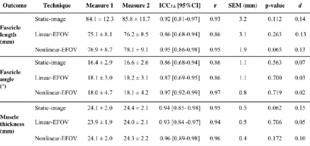
Table 2 – ICC, intraclass correlation coefficient; r, pearson's coefficient; SEM, standard error of the mean; p-value, obtained from a paired t-test; d, Cohen’s effect size ... 52

(8)

ix

INDEX OF FIGURES

Figure 1 – Identification of the three main outcomes derived from the skeletal muscle architecture assessment, from a sonogram taken at the mid-distance of the femur length, in the back of the thigh, and capturing the biceps femoris long head: deep aponeurosis, fascicle angle, fascicle length, muscle

thickness, and superficial aponeurosis ... 9

Figure 2 – Desiccation of flexor digitorum profundus to middle finger (FDPM) and ring fingers (FDPR). Image taken from Brand, Beach, and Thompson 1981 ... 15

Figure 3 – Corresponding fiber tracking of semitendinosus muscles at the mid-thigh, the left (left side) and right (right side) thighs. Image taken from Giraudo et al., 2018 ... 17

Figure 4 – (A) Schematic representation of the mechanism underlying the sonographic measurement. Image taken from Jukka Jauhiainen 2009. (B) Cross sectional area of biceps femoris long head. Image taken from Seymore et al. 2017 ... 19

Figure 5 – Sonogram obtained from the BFlh using ultrasonography. Right side corresponds to the distal component of BFlh. Image taken from Seymore et al. 2017 ... 22

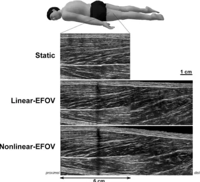
Figure 6 – Sonograms of biceps femoris long head from one individual (#13) assessed at a given region of interest using the three techniques: static-image, linear-EFOV, and nonlinear-EFOV ... 45

(9)

x

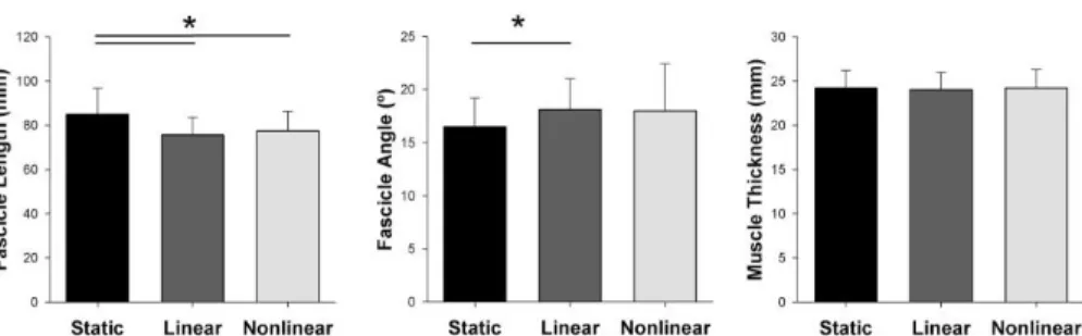
Figure 7 – Fascicle length, fascicle angle, and muscle thickness of biceps femoris (long head) assessed using static-image (static), linear-EFOV (linear), and nonlinear-EFOV (nonlinear) techniques. ……….53

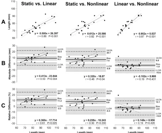
Figure 8 – Agreement of fascicle length measurements between the three sonographic techniques: Linear regression analysis (A), and Bland & Altman analysis with (B) absolute and (C) relative differences with respect to the average fascicle length obtained between the techniques (x-axis of B and C graphs)………55

Figure 9 - Agreement of fascicle angle measurements between three sonographic techniques: Linear regression analysis (A), and Bland & Altman analysis with (B) absolute and (C) relative differences with respect to the average fascicle angle obtained between the techniques (x-axis of B and C graphs)………56

(10)

xi

LIST OF ABBREVIATIONS

BF – Bicep femoris

BFlh – Bicep femoris long head EFOV – Extended field-of-view FA – Fascicle angle

FL – Fascicle length

ICC – Intraclass correlation coefficient MT – Muscle thickness

SEM – Standard error of the mean VL – Vastus lateralis

MRI – Magnetic resonance imaging DTI – Diffusion tensor imaging MTJ – Myotendinous junction ROI – Region of interest

(11)

(12)

xiii

RESUMO

Objetivo: Avaliar a repetibilidade e a concordância entre três técnicas sonográficas usadas para quantificar a arquitetura da cabeça longa do bicípite femoral (BFlh): i) imagem estática; ii) extended field-of-view (EFOV) com o caminho da sonda de ultrassom de forma linear (EFOV linear); e iii) EFOV com o percurso da sonda de forma não linear (EFOV não linear) para seguir as complexas trajetórias dos fascículos.

Método: Vinte sujeitos (24,4 ± 5,7 anos; 175 ± 0,8 cm; 73 ± 9,0 kg) sem historial de lesão nos isquiotibiais foram convidados a participar neste estudo. Foi utilizado um aparelho de ultrassom ligado a uma sonda linear de 6 cm, operando a uma frequência de 10 MHz para avaliar a arquitetura da BFlh em

B mode.

Resultados: A sonda de ultrassom foi posicionada a 52,0 ± 5,0% do comprimento do fêmur e 57,0 ± 6,0% do comprimento da BFlh. Encontramos uma repetibilidade aceitável ao avaliar o comprimento do fascículo da BFlh (ICC3,k = 0,86-0,95; SEM = 1,9-3,2 mm) e ângulo de penação (ICC3,k =

0,85-0,97; SEM = 0,8-1,1º) em todas as três técnicas sonográficas. No entanto, a técnica EFOV não linear mostrou maior repetibilidade (comprimento do fascículo ICC3,k = 0,95; ângulo de penação, ICC3,k = 0,97). A técnica de

imagem estática superestimou o comprimento do fascículo (8-11%) e subestimou o ângulo de penação (8-9%) em comparação com as técnicas de EFOV. Além disso, a ordem de classificação dos sujeitos variou em cerca de 15% entre a imagem estática e o EFOV não linear.

Conclusões: Embora todas as técnicas tenham apresentado boa repetibilidade, os erros absolutos foram observados com imagens estáticas (7,9 ± 6,1 mm para

(13)

xiv

o comprimento do fascículo) e EFOV linear (3,7 ± 3,0 mm), provavelmente porque as complexas trajetórias dos fascículos não foram acompanhadas. A ordem de classificação dos indivíduos para o comprimento e ângulo de penação também foi diferente entre a imagem estática e o EFOV não linear. Desta forma, diferentes estimativas quanto ao risco de lesão e função muscular poderiam ter sido feitas ao usar essa técnica.

Palavras chave: Ultrassonografia; repetibilidade; extended fiel-of-view; comprimento do fascículo; ângulo de penação.

(14)

xv

ABSTRACT

Purpose: To assess the repeatability of, and measurement agreement between, three sonographic techniques used to quantify biceps femoris long head (BFlh) architecture: i) static-image; ii) extended field-of-view (EFOV) with linear ultrasound probe path (linear-EFOV); and iii) EFOV with nonlinear probe path (nonlinear-EFOV) to follow the complex fascicle trajectories.

Methods: Twenty individuals (24.4±5.7 years; 175±0.8 cm; 73±9.0 kg) without history of hamstring strain injury were invited to participate in this study. An ultrasound scanner coupled with 6-cm linear probe operating at a 10-MHz frequency was used to assess BFlh architecture in B-mode.

Results: The ultrasound probe was positioned at 52.0±5.0% of femur length and 57.0±6.0% of BFlh length. We found an acceptable repeatability when assessing BFlh fascicle length (ICC3,k = 0.86-0.95; SEM = 1.9-3.2 mm) and

angle (ICC3,k = 0.85-0.97; SEM = 0.8-1.1o) using all three sonographic

techniques. However, the nonlinear-EFOV technique showed the highest repeatability (fascicle length ICC3,k = 0.95; fascicle angle, ICC3,k = 0.97). The

static-image technique overestimated fascicle length (8-11%) and underestimated fascicle angle (8-9%) compared to both EFOV techniques. Also, the rank order of individuals varied by ~15% between static-image and nonlinear-EFOV techniques when assessing the fascicle length.

Conclusions: Although all techniques showed good repeatability, absolute errors were observed using static-image (7.9±6.1 mm for fascicle length) and linear-EFOV (3.7±3.0 mm), probably because the complex fascicle trajectories were not followed. The rank order of individuals for fascicle length and angle were also different between static-image and nonlinear-EFOV, so different muscle function and injury risk estimates could likely be made when using this technique.

(15)

xvi

Key words: ultrasonography; repeatability; extended field-of-view; fascicle length; pennation angle.

(16)

1 CHAPTER I

(17)

(18)

3 CHAPTER I – INTRODUCTION

1.1. Introduction to the problem

Biceps femoris long head (BFlh) crosses the knee and hip joints posteriorly, acting as both a knee flexor, hip extensor, and tibia external rotator. BFlh also presents a complex muscle architecture, possibly because of its function complexity, which is non-uniform and heterogeneous along its length (Bennett, Rider, Domire, DeVita, & Kulas, 2014; Kellis, Galanis, Natsis, & Kapetanos, 2010). The muscle fascicles follow a nonlinear (often concave-to-convex) path, are differentially orientated along the muscle length, and most, but not all, insert onto a prominent mid-belly aponeurosis (Chleboun, France, Crill, Braddock, & Howell, 2001; Kellis, Galanis, Natsis, & Kapetanos, 2009). BFlh architecture is commonly assessed in vivo using sonographic techniques, has been statistically associated with hamstring strain injury risk (Timmins, Bourne, et al., 2016). For instance, Timmins et al. (2016) have reported that athletes with a shorter BFlh fascicle length have greater risk for sustaining a hamstring strain injury (Timmins et al., 2016). However, previous studies assessing BFlh architecture have not accounted for the complex orientation of fascicles within the BFlh belly and have used varying sonographic procedures. It is not currently known whether these fascicle length estimates are reflective of those obtained using more complex (assumedly more accurate) methods, and thus whether these associations hold true when fascicle lengths are more accurately measured.

Amongst sonographic techniques the static-image technique is the most common (Ribeiro-Alvares, Marques, Vaz, & Baroni, 2018). Using this technique on BFlh, the ultrasound transducer is typically placed at 50% of femur length, as indicated by bony landmarks (i.e. distance between the greater trochanter and the head of the fibula), and oriented according to the fascicle

(19)

4

direction between the mid-belly and superficial aponeurosis (Kellis et al., 2009; Oliveira et al., 2016; Tosovic et al., 2016; Kwah, Pinto, Diong, & Herbert, 2013). However, since BFlh has a heterogeneous and non-uniform architecture, such assessment methods may not accurately capture the fascicles for two main reasons. First, the sonogram field of view may not be sufficient to capture the full fascicle length, which necessitates the need for extrapolation techniques to estimate the non-visible portion of the fascicles. Second, BFlh fascicles follow a nonlinear path, which ensures that static-image estimates would over- (for convex curvature) or under-estimate (for concave curvature) BFlh fascicle length; and, importantly to say, previous studies using the static-image technique have assumed a linear fascicle path as they have used a straight tool to identify the fascicle path (Kellis et al., 2009; Tosovic et al., 2016; Freitas et al., 2017). To overcome such limitations, the extended field-of-view (EFOV) technique has been proposed (Cooperberg, Barberie, Wong, & Fix, 2001; Noorkoiv, Stavnsbo, Aagaard, & Blazevich, 2010). However, few studies have used the EFOV technique to assess BFlh architecture (Gonçalves et al., 2017; Seymore, Domire, DeVita, Rider, & Kulas, 2017; Tosovic et al., 2016) and these studies have either not fully described the path followed by the ultrasound transducer during image capture or have used a linear transducer path (Tosovic et al., 2016), which is not appropriate to follow nonlinear fascicle paths. Since no comparison has been performed between the different ultrasound techniques in assessing the BFlh architecture, it is unknown whether a EFOV technique using either a linear or nonlinear path would give a different BFlh architectural outcomes and repeatability compared to the static-image technique.

(20)

5

Study aim and hypothesis

The aim of the present study was to compare the repeatability of, and determine the measurement agreement between, three sonographic techniques currently used to assess BFlh architecture (i.e. fascicle length and angle): i) static-image; ii) EFOV with a linear ultrasound probe path (linear-EFOV); and iii) EFOV with nonlinear ultrasound probe path (nonlinear-EFOV). We hypothesized that i) the repeatability would be higher for the static-image technique compared to the nonlinear-EFOV and linear-EFOV technique and ii) the static-image technique would underestimate BFlh fascicle length compared to the nonlinear-EFOV technique.

(21)

(22)

7 CHAPTER II

REVIEW OF

LITERATURE

(23)

(24)

9 CHAPTER II – REVIEW OF LITERATURE

2.1. Basic Concepts of Muscle Architecture

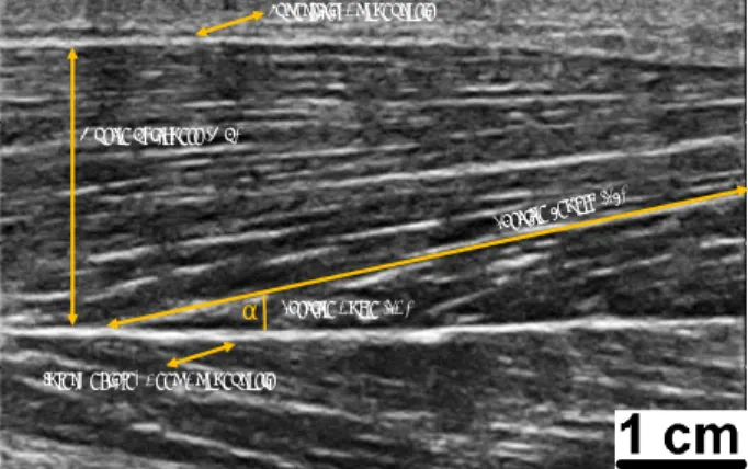
According by Otten (1988) the first work about function models and concepts of skeletal muscle architecture was published in 1664 by the Danish scientist Stensen, with a monograph entitled “Anatomical observations.” Since then, new theories and informations to analyse and interpret the skeletal muscle architecture have been developed (Brand, Beach, & Thompson, 1981). Muscle architecture is defined as the arrangement of fibers within a muscle (Gans, 1982). Although other physical parameters such as muscle mass, volume and other metabolic indicator such as fiber type distribution substantially influences the contractile properties, some authors have suggested that none predicts muscle function like the muscle architecture (Burkholder, Fingado, Baron, & Lieber, 1994; Lieber & Fridén, 2000). The arguments underlying this statement will be presented further in the present manuscript. When the muscle architecture it is the focus of the question, terms as fascicle length (FL), fascicle angle (FA) (i.e. also named pennation angle), and muscle thickness (MT) are called into the question (Fig. 1).

Figure 1. Identification of the

three main outcomes derived from the skeletal muscle architecture assessment, from a sonogram taken at the mid-distance of the femur length, in the back of the thigh, and capturing the biceps femoris long head: deep aponeurosis, fascicle angle, fascicle length, muscle thickness, and superficial aponeurosis.

Fascicle Length (FL)

Muscle Thickness (MT)

Fascicle Angle (FA) a

Superficial Aponeurosis

(25)

10

The FL and the FA are the most studied variables (Abe, Kumagai, & Brechue, 2000; Tetsuo Fukunaga, Ichinose, Ito, Kawakami, & Fukashiro, 1997; Kawakami, Abe, & Fukunaga, 1993; Otten, 1988; Rutherford & Jones, 1992). However, there is a certain discrepancy in previous studies regarding the method used to perform the measurements. For instance, for the FL measurements in vastus lateralis, (T. Fukunaga, Kawakami, Kuno, Funato, & Fukashiro, 1997) determined the FL as the length of a line drawn along the ultrasonic echo parallel to fascicles (which was considered as fibers as well), from their proximal and distal ends. On other hand (Abe et al., 2000), determined the fascicle length from a formula which included the isolate muscle thickness (i.e. distance between subcutaneous adipose tissue-muscle interface and intermuscular interface) and fascicle angle (1):

FL= isolated muscle thickness • sin-1 ₍₁₎

For Tosovic, Muirhead, Brown, & Woodley (2016), the FL of BFLh was defined as the length of an entire muscle fascicle that extends from the superficial aponeurosis to the deep intramuscular aponeurosis. In this document, the FL was considered as a group of fibers involved by a perimysial conjunctival fraction that extends between two aponeuroses. Therefore, the FL length was considered as the distance between the insertions of the FL onto the aponeurosis by following the FL path. Important to note that as the FL orientation implies the orientation of the muscle fibers that it contains, FL may be considered an estimator of fiber length.

In respect to the FA assessment, previous studies have also used different criteria when assessing different muscles. Fukunaga in 1997 considered the FA was the angle between the echoes of the deep aponeurosis of the vastus lateralis and the echoes from interspaces among fascicles (Tetsuo Fukunaga et al.,

(26)

11

1997; Otten, 1988). Other studies also used this definition (Abe et al., 2000; Tetsuo Fukunaga et al., 1997; Kawakami et al., 1993; Rutherford & Jones, 1992). In other perspective, other studies digitized two points on each fascicle, one 3 mm from the deep aponeurosis and the second at 50% of the distance from the deep to superficial aponeurosis (Blazevich, Cannavan, Coleman, & Horne, 2007; Timmins, Shield, Williams, Lorenzen, & Opar, 2015). As mentioned by the studies authors, this allowed accurate delineation of the fascicles without incorporating the slightly greater fascicle curvature that can occur at the insertion point of the fascicles on the deep aponeurosis. For Tosovic et al. (2016), the fascicle angle was defined as the angle between the superficial aponeurosis and a clearly visible fascicle, measured using the angle tool of the ImageJ software (National Institutes of Health, Bethesda, MD), without precising where fascicle was digitized. This indicates that a different aponeurosis could be considered when assessing the FA, as well the sites where the fascicle is digitized. In this study, we describe the FA as the angle between the fascicle orientation (i.e. defined by the most superficial and deep insertions sites onto the aponeuroses) and the deep aponeurosis, considering that the aponeurosis is aligned to the muscle line of action during contraction (Timmins, Shield, Williams, Lorenzen, & Opar, 2015). The aponeurosis is defined as a multilayered structure with densely laid down bundles of collagen with major preferential directions, that extends from the tendon, and contains insertions of muscle fascicles (Huijing PhD, Huijing, & Langevin, 2009). Note that the epimysium also covers the aponeurosis but is not attached to them.

The arrangement of the muscle fibers and them insertion (or not) in the aponeurosis, modified the name of type for muscle architecture. The human skeletal muscle can be described as either parallel or pennate. In parallel muscles, the fibers run parallel to the line of pull of the muscle. In pennate muscles, fibers run obliquely to the axis of pull and insert into the aponeurosis

(27)

12

or tendon by forming an angle, called the FA or pennation angle (M. Narici, 1999). The FA, and the amount of force actually exerted on the tendon, can be calculated using the cosine of the angle of insertion. At rest, the angle of pennation in most human muscles is about 10° or less and does not appear to have a marked effect on most functional properties such as force production (Wickiewicz, Roy, Powell, & Edgerton, 1983; Wickiewicz, Roy, Powell, Perrine, & Edgerton, 1984). However, during muscle contraction the FA can vary and may change some functional parameters, at least in some muscles (Tetsuo Fukunaga et al., 1997). The pennate muscles offers a force advantage over parallel muscles, because with pennation there are more fibers in parallel for a given muscle volume, which increases the physiological cross sectional area (the area of the cross section of a muscle perpendicular to its fibers, generally at its largest point). This allows to have more sarcomeres to be arranged in parallel, resulting in enhanced force production (Gans & Gaunt, 1991; Sacks & Roy, 1982). From a functional perspective, is important to note that the force exerted by muscle fibers is modified by their geometric arrangement, structures of the joint, the angle and location of the tendon in relation to the bone (Gans & de Vree, 1987).

There are some methodological considerations when assessing the FA and FL in human skeletal muscles. For instance, the FA and FL measurement depends on the degree of muscle lengthening and muscle activity (Huijing, 1985; Muhl, 1982). Thus, it is fundamental to control for the degree of muscle activation and joint positioning during the FL and FA assessments. Also, previous studies reported the fascicles may present curvatures at rest (Blazevich et al., 2007; Tetsuo Fukunaga et al., 1997; Noorkoiv, Stavnsbo, Aagaard, & Blazevich, 2010); and, in some cases, a doubled curvature can exist (Bolsterlee, D’Souza, Gandevia, & Herbert, 2017).

(28)

13

The MT has been defined as the perpendicular distance between two aponeuroses within a muscle (Blazevich et al., 2007; Timmins et al., 2015). This parameter reflects muscle size. Previous studies have demonstrated that the muscle size, determined as anatomical or physiological cross-sectional area and muscle volume, is closely related to the maximal voluntary strength in isometric contractions (R. Akagi et al., 2009; Ryota Akagi et al., 2011; Maughan, Watson, & Weir, 1983).

2.2. Overview of Current Methods

In order to answer the problems of measuring muscular architecture, science has evolved over the years. The first skeletal muscle architecture measurements have been made with ex vivo animal models. According to Denny-Brown (1929) the dissection on animals started at 1678 with Stefano Lorenzini, which mentioned the striking difference in colour between certain muscles of the limb in the rabbit. After that, and according to Friederich & Brand (1990), new important studies have been published regarding the cross sectional area assessment, as the Weber work in 1846. The type of animal models to be dissected has varied along the time, using animals as rats, cats, and kangaroos (Close, 1964; Denny-Brown, 1929; Hoffer, Caputi, Pose, & Griffiths, 1989; Morgan, Proske, & Warren, 1978); and, only years after, started to be performed assessments in skeletal muscles of human cadavers (Fig.2) (Brand et al., 1981; Friederich & Brand, 1990; Wickiewicz et al., 1983). The dissection was the first method developed to analyse the muscle architecture. This method consists on the dismembering of the body of a deceased (i.e. animal, plant or human) to study the anatomy. The main advantage of the dissection is that allows to understand and visualize in loco

(29)

14

the composition/tissues of the body by avoiding structures that should not be evaluated (Friederich & Brand, 1990). On the other hand, the dissection only allows to use one time the dissected animals (i.e. when the animals are sacrificed or have to be deeply anaesthetized) (Hoffer et al., 1989; Morgan et al., 1978). In humans, the dissection must be previously allowed in order to have assess and examine human cadavers, depend (of course) of their availability, and most of them are older (Friederich & Brand, 1990; Tosovic, Muirhead, Brown, & Woodley, 2016b; Wickiewicz et al., 1983).

In the middle of the 20th_{century, the sonography was proposed to be}

appropriate to assess the skeletal muscle architecture in vivo, and non-invasively (Ikai & Fukunaga, 1968). To our knowledge, (Ikai & Fukunaga, 1968) reported the first sonographic study that proposed to assess the skeletal muscle morphology, measuring the cross section area. Since then, the quality of ultrasound measures have improved (Gary S. Chleboun, France, Crill, Braddock, & Howell, 2001; Dons, Bollerup, Bonde-Petersen, & Hancke, 1979; Tetsuo Fukunaga et al., 1997; Heckmatt, Dubowitz, & Leeman, 1981; Noorkoiv et al., 2010) until now (Kellis, 2018; Seymore, Domire, DeVita, Rider, & Kulas, 2017; Tosovic et al., 2016). Currently, the ultrasonography is considered an usual and appropriate method in medicine (by using echo waves through high frequency ultrasound) to visualize, in real time, the internal structures of the body.

(30)

15

Figure 2. Desiccation of flexor digitorum profundus to middle finger (FDPM) and ring

fingers (FDPR). Image taken from Brand, Beach, and Thompson 1981.

Parallel to the ultrasound measurements, discoveries of muscle architecture have been also performed using magnetic resonance imaging (Cleveland, Chang, Hazlewood, & Rorschach, 1976). The magnetic resonance imaging (MRI) is currently widely considered to be the gold standard for the muscle morphological assessment in vivo due to the high contrast between tissues of different molecular properties, by using the diffusion tensor imaging (DTI) (P. J. Basser, Mattiello, & LeBihan, 1994). The measurement of an effective diffusion tensor of water in tissues can provide clinically relevant information that is not available from other imaging modalities (Peter J. Basser & Jones, 2002). This information includes parameters that help to characterize physical

(31)

16

properties of tissue constituents, tissue microstructure, and architectural organization.

Thus, the DTI provides a good approach for determining the muscle shape and the orientation of the muscle fibers, which are assumed to be similar to the fascicles (Fig.3) (Budzik et al., 2007; Giraudo et al., 2018). DTI is based on the correspondence between the principal direction of water diffusion and the local cellular geometry in tissues such as skeletal muscle (Cleveland et al., 1976; Damon, Ding, Anderson, Freyer, & Gore, 2002; Henkelman, Mark Henkelman, Stanisz, Kim, & Bronskill, 1994), cardiac muscle (Wu et al., 2006), the white matter tracts of the central nervous system (P. J. Basser & Pierpaoli, 1996), and have found clinical application in neuroradiology (Yang, Zhang, Zhang, Zhao, & Zhao, 2006). It has been demonstrated that DTI fiber tracking is feasible in human muscle studies as well (Sinha, Sinha, & Edgerton, 2006). DTI may additionally be useful for studies of the musculoskeletal field (Budzik et al., 2007) as muscle microarchitecture, with potential sensitivity to such parameters as fiber diameter (Galbán, Maderwald, Uffmann, de Greiff, & Ladd, 2004; Saotome, Sekino, Eto, & Ueno, 2006), and muscle injury (Heemskerk et al., 2006; Zaraiskaya, Kumbhare, & Noseworthy, 2006). So DTI, offers great potential for understanding structure-function relationships in human skeletal muscles (Lansdown, Ding, Wadington, Hornberger, & Damon, 2007). However, the access to DTI for research purposes is often limited due to the large clinical demand and the considerable cost. Consequently, other alternative methods, as sonography, is more often used.

(32)

17

Figure 3. Corresponding fiber tracking of semitendinosus muscles at the mid-thigh, the

left (left side) and right (right side) thighs. Image taken from Giraudo et al., 2018.

2.3. Assessment using Sonography

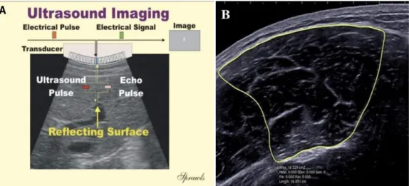
The diagnostic sonography (ultrasonography) is an imaging technique used to visualize subcutaneous body structures including tendons, muscles, joints, vessels and internal organs for possible pathology or lesions. The mechanism underlying the sonography is complex. Briefly, the ultrasound machine incorporates a transducer to perform the scans that originates the sound to be transmitted with a very high frequency into the body. A water-based gel is often placed between the patient's skin and the probe in order to improve the acoustic condition. The sound wave generated when propagates into the tissues is partially reflected from the layers between different tissues. Specifically, sound is reflected anywhere there are density changes in the body (e.g. blood cells in blood plasma, small structures in organs, etc). Some of the reflections return to the transducer. The return of the sound wave to the transducer results in the same process that it takes to emit the sound wave, but with an opposite direction. The return of the sound wave vibrates the transducer, and the transducer converts the vibrations into electrical pulses that travel to the ultrasonic scanner where they are processed and transformed into a digital image (Fig. 4-A) (Jauhiainen, 2009).

(33)

18

Typical diagnostic sonographic scanners operate in the frequency range of 2 to 18 megahertz (MHz), which is hundreds of times greater than the limit of human hearing. Note that, if the frequency is higher, more superficial tissues will be the scanned. For the assessment of muscle architecture, the probe normally operates at 10-12 MHz (Freitas, Marmeleira, Valamatos, Blazevich, & Mil-Homens, 2017; Kellis, 2018; Timmins, Bourne, et al., 2016a; Timmins et al., 2015). The sonography has been the front-line technique for investigating musculoskeletal architecture in different areas, because of its accessibility and reduced cost (Connell et al., 2004).

Ultrasonography has been used to measure changes in MT (Hides, Stokes, Saide, Jull, & Cooper, 1994; Misuri et al., 1997), FA (Herbert & Gandevia, 1995; Maganaris & Baltzopoulos, 1999), and FL (McKenzie, Gandevia, Gorman, & Southon, 1994; M. V. Narici et al., 1996), in different conditions as during static and dynamic contractions (Blackburn, Troy Blackburn, & Pamukoff, 2014; Ribeiro-Alvares, Marques, Vaz, & Baroni, 2018; Cepeda, Lodovico, Fowler, & Rodacki, 2015; Hodges, Pengel, Herbert, & Gandevia, 2003; Timmins, Bourne, et al., 2016b; Timmins, Shield, Williams, Lorenzen, & Opar, 2015), or during passive muscle stretching (Kellis, 2018; Nakamura, Ikezoe, Takeno, & Ichihashi, 2013). Ultrasonography has also been suggested to be able to noninvasively record the activity from deep muscles without crosstalk from adjacent muscles; but, with limited data to validate such proposal (Hodges et al., 2003). The ultrasonography method is a valid and reliable alternative tool for assessing cross-sectional areas of large individual human muscles (Reeves, Maganaris, & Narici, 2004), with the probe in a transversal position to the muscle length (Fig. 4-B). This technique, however, is not of sufficient quality to allow delineation of individual muscles (Reeves et al., 2004). The FL and FA are two architectural variables that are readily

(34)

19

measured using ultrasound imaging. But, to not interfere with the results, little pressure on the skin should be made by the probe (Gary S. Chleboun et al., 2001). Here, the probe should be positioned in a longitudinal plan in relation to the muscle length as is shown above in figure 1. Previous studies have demonstrated that the ultrasound measurement of FA is underestimated, when compared to assessment using a DT-MRI technique (Bolsterlee, Veeger, van der Helm, Gandevia, & Herbert, 2015).

Figure 4. (A) Schematic representation of the mechanism underlying the sonographic

measurement. Image taken from Jukka Jauhiainen 2009. (B) Cross sectional area of biceps femoris long head. Image taken from Seymore et al. 2017.

2.4. Biceps Femoris Long Head

2.4.1. Clinical Relevance

Hamstring strains are common injuries in sport, particular in those who involve sprinting and jumping (Garrett, Califf, & Bassett, 1984; Stanton & Purdam, 1989). For instance, (Woods et al., 2004) reported a detailed analysis in English professional football players over two seasons, which 12% of all

(35)

20

injuries reported were hamstring strains, this being the most prevalent injury. Athletes were 2.5 times more likely to sustain a hamstring strain than a quadriceps strain during a game (Woods et al., 2004). Of the total injuries over the two seasons, nearly half (i.e. 53%) involved the biceps femoris (Woods et al., 2004). Most strains in dynamic movements of the lower limb are reported to occur in the BFlh (Brockett, Morgan, & Proske, 2004; Hoskins & Pollard, 2005; Orchard, Seward, & Orchard, 2013; Proske, Morgan, Brockett, & Percival, 2004), and the majority are recurrent (Croisier, Forthomme, Namurois, Vanderthommen, & Crielaard, 2002; Orchard et al., 2013; Verrall, Slavotinek, Barnes, Fon, & Esterman, 2006). Nonetheless, the hamstring strain injuries represent between 11 and 21.5% of the total injuries in soccer and up to 84% of the strains involved the biceps femoris, particularly the long head, while semimembranosus and semitendinosus were affected in 12% and 4% of the cases, respectively (Ekstrand, Lee, & Healy, 2016; Turner et al., 2014; Woods et al., 2004a). The region more affected is reported to be the proximal component, near to the MTJ (De Smet & Best, 2000; Silder, Heiderscheit, Thelen, Enright, & Tuite, 2008; Silder, Reeder, & Thelen, 2010).

Several factors are reported to increase the likelihood of hamstrings strains, including their two-joint anatomy and their forceful activation during eccentric contractions (Opar, Williams, & Shield, 2012; Thelen et al., 2005). Despite the frequency of hamstring muscle injuries during sprinting, it remains unclear when in the gait cycle the muscle is injured or why the BFlh is more susceptible to injury. Late swing (Wood, 1987) and early stance phases (Mann & Sprague, 1980) of sprinting have been suggested as potentially injurious phases of the gait cycle. During late swing, the hip is flexed, and the knee is extending. The hamstring muscles are active at this stage (Kuitunen, Komi, & Kyröläinen, 2002; Mero & Komi, 1987) while lengthening, which could induce an eccentric contraction injury (Garrett, 1996). Therefore, (Thelen et al., 2005)

(36)

21

analysis the kinematics of the hamstring muscles during treadmill sprinting and concluded that intermuscle differences in hamstring moment arms about the hip and knee may be a factor contributing to the greater propensity for hamstring strain injuries to occur in the BFlh.

An unresolved issue with hamstring strain injury is the elevated risk of recur. It has been suggested that a premature return to play (Croisier et al. 2002; Agre 1985; Jönhagen, Németh, and Eriksson 1994), or an inappropriate rehabilitation programme (Croisier et al. 2002; Agre 1985; Bennell et al. 1998), may be responsible for reinjury. But, BFlh architecture has also been statistically associated for the strain injury risk (Seymore, Domire, DeVita, Rider, & Kulas, 2017; Thelen et al., 2005; Woods et al., 2004). A previous study reported shorter fascicles have previously been associated a greater risk of injury (Timmins, Bourne, et al., 2016). Here, the eccentric strength training has became an effective method for prevention (Arnason, Andersen, Holme, Engebretsen, & Bahr, 2008; Askling, Karlsson, & Thorstensson, 2005), since it been demonstrated to increase FL and to reduce FA (Potier, Alexander, & Seynnes, 2009; Timmins, Ruddy, et al., 2016).

2.4.2. General Anatomy

Morphological data pertaining to BFlh have been reported in several studies (Kellis, Galanis, Natsis, & Kapetanos, 2010; Makihara, Nishino, Fukubayashi, & Kanamori, 2005; Seidel, Seidel, Gans, & Dijkers, 1996; van der Made et al., 2015; Woodley & Mercer, 2005). However, few have focused on segmental architecture (Kellis et al., 2010; Woodley & Mercer, 2005), and most data have been derived from linear measures in cadaver specimens.

(37)

22

The BFlh posteriorly crosses the knee and hip joints, with the proximally insertion in the ischial tuberosity and insert distally on the head of the fibula. Acts as both a knee flexor, hip extensor, and tibia external rotator. BFlh consists of two regions, a surface and a deeper one, arranged in parallel, that is separated by a mid-aponeurosis (Woodley & Mercer, 2005). BFlh presents a complex muscle architecture, which is non-uniform and heterogeneous (Bennett, Rider, Domire, DeVita, & Kulas, 2014; Kellis et al., 2010). The muscle fascicles have a non-linear path at rest and a different orientation along the muscle length, and most, but not all, fascicles inserting onto the mid-belly aponeurosis (G. S. Chleboun, France, Crill, Braddock, & Howell, 2001a; Kellis, Galanis, Natsis, & Kapetanos, 2009). The architecture of BFlh is heterogeneous in relation to the entire length of the muscle (Fig.5), by having a different behavior at different muscle activation levels (Bennett et al., 2014). Fascicles are more longer, and the FA are greater in the proximal region, compared to the distal region (Seymore et al., 2017). At rest (i.e. non-contracted condition), fascicles are thought to be curved and oriented in three planes (Freitas et al., 2017; Froeling et al., 2015). The highest BFlh cross-sectional area and muscle thickness can be found between 40-60% of the muscle length (Seymore et al., 2017).

Figure 5. Sonogram obtained from the BFlh using ultrasonography. Right side

(38)

23

2.4.3. Architecture

As already reported in the previous topic, and assuming the complexity of BF, previous studies reported that longitudinal mid-muscle aponeurosis extends from the proximal to the distal MTJ, onto which superficial fascicles insert (Kellis, Galanis, Natsis, & Kapetanos, 2009. At rest, this aponeurosis presents a non-linear path, even though the superficial BF aponeurosis follows a linear path for most of the length of the muscle belly. The proximal and distal BFlh tendon junctions have a different morphology. The distal BF muscle-tendon junction is superficial, close to the skin, and its most distal point is easily observed as it ends proximal to the biceps femoris (Freitas et al., 2017). The proximal BF muscle-tendon junction is located deep, merges medially onto the semitendinosus tendon and together insert onto the ischial tuberosity.

Tosovic in 2016 measured the BFlh using a human cadaver specimen and ultrasound reported that muscle architecture was variable throughout the BFlh length. Of note, the distal-most part of the muscle (i.e. at 90% of muscle length) contained shorter fascicles which were more pennated than its proximal most site (i.e. at 30% of muscle length). This arrangement of fascicles is typical of muscles designed for force production, as the pennated orientation allows for a relatively greater number of fascicles to be packed in the muscle, parallel to each other (Aagaard et al., 2001; Wickiewicz et al., 1983). This finding is contradictory to what was reported by (Seymore et al., 2017). This might be related to a different sonographic method used between studies. While a linear-EFOV technique was used in Tosovic (2016) study, the Seymore (2017) study do not reported the technique. Consequently, and according to (Tosovic et al., 2016) work, it appears that the proximal segment of BFlh has larger fascicle excursion potential compared to its distal region. When all the muscle architecture parameters (i.e FL, FA, and MT) were compared between the

(39)

24

cadaver specimens to the ultrasound measurements, lower values was noted (Tosovic et al., 2016). This could be attributed to the dehydration of the tissues.

2.4.4. Sonographic Considerations in Assessing the Architecture

The static-image technique is the most common to assess the BFlh architecture (Ribeiro-Alvares, Marques, Vaz, & Baroni, 2018). Using this technique, the ultrasound transducer is typically placed at 50% of femur length, as indicated by bony landmarks (i.e. distance between the greater trochanter and the head of the fibula), and usually oriented according to the fascicle direction between the superficial and mid-belly aponeurosis (Kellis, Galanis, Natsis, & Kapetanos, 2009; Oliveira et al., 2016; Tosovic et al., 2016). However, as the sonogram field of view may not be sufficient to capture the full fascicle length, and BFlh fascicles at rest have a non-linear path, the extended field of view (EFOV) technique has been proposed (Cooperberg, Barberie, Wong, & Fix, 2001; Noorkoiv et al., 2010). (Noorkoiv et al., 2010) have demonstrated a very high repeatability for the assessment of vastus lateralis FL using the EFOV ultrasonography technique.

Table 1 shows the methods and general procedures reported in previous studies that assessed the BFlh architecture using sonography, and some methodological considerations. Few studies have used the EFOV technique to assess the BFlh architecture (Bennett et al., 2014; Gonçalves, Hegyi, Avela, & Cronin, 2017; Seymore, Domire, DeVita, Rider, & Kulas, 2017c; Tosovic et al., 2016). And, these studies have either not fully described the path followed by the ultrasound transducer during image capture (Bennett et al., 2014; Gonçalves et al., 2017; Seymore et al., 2017), or have used a linear transducer path (Tosovic et al., 2016), which is not appropriate to follow nonlinear

(40)

25

fascicle paths. Some researchers (Gary S. Chleboun et al., 2001; Kellis et al., 2009) used a collection of images along the length of the muscle with static-image technique to reproduce all the architecture of BFlh. Regarding the location of imaging within the muscle, the region of interest (ROI) used to examine BFlh architecture has varied substantially between previous studies.

(41)

26

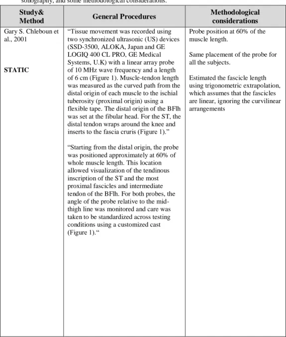
Table 1. Summary of the sonographic method, general procedures described in

previous published studies that assessed the biceps femoris long head architecture using sonography, and some methodological considerations.

Study&

Method General Procedures

Methodological considerations

Gary S. Chleboun et al., 2001

STATIC

“Tissue movement was recorded using two synchronized ultrasonic (US) devices (SSD-3500, ALOKA, Japan and GE LOGIQ 400 CL PRO, GE Medical Systems, U.K) with a linear array probe of 10 MHz wave frequency and a length of 6 cm (Figure 1). Muscle-tendon length was measured as the curved path from the distal origin of each muscle to the ischial tuberosity (proximal origin) using a flexible tape. The distal origin of the BFlh was set at the fibular head. For the ST, the distal tendon wraps around the knee and inserts to the fascia cruris (Figure 1).”

“Starting from the distal origin, the probe was positioned approximately at 60% of whole muscle length. This location allowed visualization of the tendinous inscription of the ST and the most proximal fascicles and intermediate tendon of the BFlh. For both probes, the angle of the probe relative to the mid-thigh line was monitored and care was taken to be standardized across testing conditions using a customized cast (Figure 1).“

Probe position at 60% of the muscle length.

Same placement of the probe for all the subjects.

Estimated the fascicle length using trigonometric extrapolation, which assumes that the fascicles are linear, ignoring the curvilinear arrangements

(42)

27

Study&

Kellis et al., 2009

STATIC

“US images were taken with the probe at approximately 10%, 30%, 50% and 70% of the curved path from the distal MTJ to the proximal origin. The angle of the probe relative to the mid-thigh line was monitored and it was standardized for all specimens.”

Images in different places are better that only one image to represent all muscle length, but this method isn’t valid for muscle architecture. Associated a major error.

Estimated the fascicle length using trigonometric extrapolation, which assumes that the fascicles are linear, ignoring the curvilinear arrangements.

Potier, Alexander, & Seynnes, 2009

STATIC

“The ultrasound probe (41mm, LA424 14 8, Genova, Italy) was placed on the skin overlying the distal part of the biceps femoris and its position was recorded in order to be able to replace the probe in the same position after the 8-week training period was completed. The position of the probe was recorded by measuring the distance from a fixed point on the probe to the posterior

margin of the iliotibial band, the greater trochanter and the tibial condyle.”

“Sections of FL that were not visible on the image were extrapolated as a straight line (Maganaris et al. 1998; Narici et al. 1996), and the summation of measured and extrapolated FL was calculated to obtain total FL.

Not reported the localization of the ROI in relation to the bone and muscle length to compare the results.

(43)

28

Study&

Blackburn et al., 2014

STATIC

“Still ultrasonic images (Sonosite M-Turbo, Sonosite, Inc., Bothell, WA, USA) were obtained from the biceps femoris long head 50% of the distance between the greater trochanter of the femur and the lateral knee joint line with the muscle in a relaxed state.”

Reported the probe position in relation to the muscle.

Cepeda, Lodovico, Fowler, & Rodacki, 2015

STATIC

“Since the probe was not long enough to measure fascicle length in a single image, four images of each muscle were taken and grouped.”

“For the BF, the images were obtained from a site at 33% of the segment length (from the great trochanter to the articular knee line).”

Images in different places are better that only one image to represent all muscle length, but this method isn’t valid for muscle architecture. Associated a major error.

Not argue the choose of ROI site.

Not reported any image for BFlh.

(44)

29

Study&

e Lima et al., 2015

STATIC

“The probe was placed at 50% of thigh length, defined as the distance from the greater trochanter to the popliteal crease.”

“When the FL exceeded US field of view, FL was calculated by the extrapolation of a straight line that was summed to the visible FL, as proposed by Potier et al. Pennation angle was calculated as the acute angle formed between the deep aponeurosis and a muscle fascicle.”

Use a bonymark reference and a other anatomical line.

Freitas & Mil-Homens, 2015

STATIC

“A classic linear extrapolation method was used to calculate the BF architecture parameters (11). The FL was calculated using the equation: FL = L +(h/sin), where L is the observable FL from the mid-muscle aponeurosis to the most visible end point, h is the distance between the superficial aponeurosis and the fascicle visible distal end point, and b is the angle between the fascicle (drawn linearly) and the superficial aponeurosis (Figure 1B).”

Choose the most clearly area for different subjects and not the same position for all.

Not reported the localization of the probe.

(45)

30

Study&

Timmins et al., 2015

STATIC

“The scanning site was determined as the halfway point between the ischial tuberosity and the knee joint fold, along the line of the BFlh. Once the scanning site was determined, the distance of the site from various anatomical landmarks was recorded to ensure reproducibility of the scanning site for future testing sessions.”

“To gather ultrasound images, the linear array ultrasound probe, with a layer of conductive gel, was placed on the skin over the scanning site, aligned longitudinally and perpendicular to the posterior thigh.”

Use a bony mark reference and a anatomical line.

(46)

31

Study&

Method General Procedures Methodological considerations

Kellis, 2016

STATIC

“Tissue movement was recorded using two synchronized ultrasonic (US) devices (SSD-3500, ALOKA, Japan and GE LOGIQ 400 CL PRO, GE Medical Systems, U.K) with a linear array probe of 10 MHz wave frequency and a length of 6 cm (Figure 1). Muscle-tendon length was measured as the curved path from the distal origin of each muscle to the ischial tuberosity (proximal origin) using a flexible tape. The distal origin of the BFlh was set at the fibular head. For the ST, the distal tendon wraps around the knee and inserts to the fascia cruris (Figure 1).” “Starting from the distal origin, the probe was positioned approximately at 60% of whole muscle length. This location allowed visualization of the tendinous inscription of the ST and the most proximal fascicles and

intermediate tendon of the BFlh. For both probes, the angle of the probe relative to the mid-thigh line was monitored and care was taken to be standardized across testing conditions using a customized cast (Figure 1).“

Probe position at 60% of the muscle length.

Estimated the fascicle length using trigonometric extrapolation, which assumes that the fascicles are linear, ignoring the curvilinear

(47)

32

Study&

Oliveira et al., 2016

STATIC

“The examiner marked one point at 50% of the length of the thigh, determined by the distance between the greater trochanter and head of the fibula.”

“The probe was positioned along the direction of the fascicles, where the fascicular organization between the superficial and deep aponeurosis on the muscle was better visualized.”

Only had in consideration the length of the bone and not reported % in relation to the length of the muscle.

arrangements.

Sá et al., 2016

STATIC

“The volunteers rested in the supine position on a stretcher. Longitudinal US images of the vastus lateralis (VL) and biceps femoris (BF) were acquired at 50% of the thigh length of the dominant leg by an experienced examiner.”

Not reported any image of BFlh, only the VL.

(48)

33

Study&

Timmins, Bourne, et al., 2016

STATIC

“The scanning site was determined as the halfway point between the ischial tuberosity and the knee joint fold, along the line of the BFlh. Once the scanning site was

determined, the distance of the site from various anatomical landmarks was recorded to ensure reproducibility of the scanning site for future testing sessions.”

Use a bony mark reference and a anatomical line.

arrangements. Alonso-Fernandez, Docampo-Blanco, & Martinez-Fernandez, 2017 STATIC

“MT, FA and the estimation of FL were determined from ultrasound images obtained along the longitudinal axis of the muscle belly using a 2D B-mode

ultrasound.”

“The measurement site was the halfway point between the ischial tuberosity and the posterior knee joint fold, along the line of the BFlh. Once the scanning site was determined in each participant, several anatomical landmarks were taken (ischial tuberosity, fibula head and midpoint of the posterior knee joint fold) and photographs were taken in order to ensure

reproducibility for future assessment sessions.”

Use a the insertion of BFlh as reference and a anatomical line.

(49)

34

Study&

Ribeiro-Alvares, Marques, Vaz, & Baroni, 2018

STATIC

“The scanning site for the BFlh was determined as the halfway point between the ischial tuberosity and the superior border of the fibular head.”

“If necessary, slight adjustment in the probe orientation was made by the examiner in order to optimise the fascicle

identification.”

“Because fascicle length was greater than the probe surface, the nonvisible part was estimated through a trigonometric function.”

Placement of the probe according to the length of the bone.

arrangements.

Freitas et al., 2017

STATIC

“The ROI was chosen in the most clearly area, capturing the superficial and mid-muscle aponeurosis and BF fascicles was obtained.”

“Fascicle length was calculated using the equation: FL=L + (h/sinβ).”

Choose the most clearly area for different individuals and not the same position for all.

The static mode it is more reproducible, because the sonograms are always taken in the same position of the ROI, only variate the probe inclination but do not analyse all fascicle length.

The sonogram field of view it is not sufficient to capture the full fascicle length, which necessitates the use extrapolation techniques to estimate the non-visible component of the fascicles.

(50)

35

Study&

Kellis, 2018

STATIC

“This location allowed visualization of the most distal fascicles and intermediate tendon of the BFlh. Further, it was selected because distal fascicles are shorter [Kellis et al., 2012] and therefore easier to measure using US.”

“In contrast, in the present study FL was determined from the distal area of the muscle using geometry estimation from US marker position data during slow passive knee joint motion. It is therefore, clear, that further research on changes in BFlh architectural parameters at various joint positions is necessary.”

The location of the probe it’s to much external (image in the study).

Collection of images in different regions.

Only analyze the region where the fascicles are shorter.

arrangements.

Seymore et al., 2017

—

“Cross-sectional images were acquired along the length of the muscle at 11 equidistant points from the most distal cross-sectional image of the muscle that could be traced and measured, which is just proximal to the musculotendinous junction, to the gluteal fold; encompassing 0–100% of the visualized muscle length. Two images for each of the 11 cross-sectional points were recorded. Two longitudinal images were then recorded to allow for the estimation of fascicle length and pennation angle.”

Not reported the methodology used (linear-EFOV or non-linear EFOV).

Not reported the localization of the ROI site, in relation to the bone or muscle.

Not indicate the path and orientation of the probe.

(51)

36

Study&

Tosovic et al., 2016

LINEAR EFOV /STATIC

“.. along with the most proximal and distal extents of muscle fiber insertion onto the proximal and distal tendons respectively, were scanned and the position of each was marked on the skin. Using these skin markings the following lengths were recorded with a flexible tape measure.”

“Additional scans were taken

systematically, at four points along BFlh, namely at 30, 50, 70, and 90% of the total muscle length.”

“Still ultrasound images were also taken with the probe aligned along the long axis of BFlh, and these images were imported as DICOM files into ImageJ (National

Institutes of Health, Bethesda, MD) for analysis of FL and FA (undertaken by DT) (Fig. 1B).

Fascicle length was defined as the length of an entire muscle fascicle that extended from the superficial aponeurosis to the deep intramuscular aponeurosis and was calculated by setting the appropriate scale and using the “straight line tool” in imageJ software.”

In the linear method, assumes a linear orientation for the FL, but the FL are curve.

In the static method, estimated the fascicle length using trigonometric extrapolation, which assumes that the fascicles are linear, ignoring the curvilinear arrangements.

(52)

37

Study&

Bennett et al., 2014

NON-LINEAR EFOV

“First, the full length of the muscle was measured twice on each image using digital calipers, starting at the most proximal point of the muscle before the musculotendinous junction, and ending at the most distal point of the muscle.”

“Two fascicles were measured in each region of the BFlh, starting at the fascicle's superﬁcial origin and ending at the fascicle's insertion onto the deep aponeurotic tendon.”

“As the transducer was removed between contractions, measured fascicles are likely not the same fascicles, but are within a speciﬁed region of fascicles.”

Only perform 2 sonograms along the total length of the muscle and trace in the sonogram a line at 50% for the total length of the field of view.

Do not guarantee that analyse the same fascicles in the two scans.

Not reported the path and orientation of the probe and if the orientation is according to the FL.

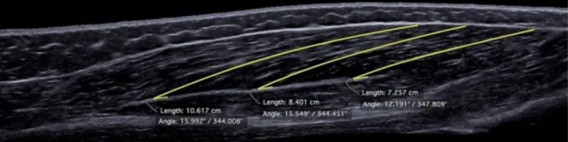
Gonçalves et al., 2017

NON-LINEAR EFOV

“Three regions of the muscle were defined using as a reference the shadow of the reflective tape and 4 fascicles for each region were digitized in the image (FIGURE 3). Only distal and middle regions of the muscle were used due to the poor quality of the images. The line was digitized from the superficial aponeurosis and the fascicles were followed until the deep aponeurosis.

In case of having images with curved fascicles, they were tracked in a series of connected lines.”

Not report which % was the ROI in relation to the muscle length. Not follow the orientation of the fascicles.

Reported that the use of EFOV ultrasound technique shows to be highly reliable to measure FL but poor to measure PA and MT. Affirmed that is a valid method to measure directly FL of the BF in future research.

Reported poor quality of the images.

Legend: Fascicle length (FL); Fascicle angle (FA); Muscle Thickness (MT); Bicep

femoris long head (BFlh); Vastus lateralis (VL); Ultrasound (US); Region of interest (ROI).

Probe Position

Regarding the probe positioning used in the previous studies (Table 1), different anatomical criteria have been used to identify the BFlh region of

(53)

38

interest, including (i) the mid-distance (i.e. 50%) between the ischial tuberosity and the knee joint fold (Alonso-Fernandez et al., 2017; Timmins, Bourne, et al., 2016; Timmins, Shield, Williams, Lorenzen, & Opar, 2015), (ii) between the greater trochanter and head of the fibula (Oliveira et al., 2016b), (iii) between the greater trochanter and the lateral knee joint line (Blackburn et al., 2014), and (iv) between the greater trochanter and the tibial condyle (Potier, Alexander, & Seynnes, 2009). Additionally, studies have used different percentages of the distance between the anatomical landmarks, such as 33% (Cepeda et al., 2015), or 10%, 30%, 50% and 70% (Kellis, Galanis, Natsis, & Kapetanos, 2009). Previous research performed using human cadavers has shown that the distal region of BFlh presents shorter fascicles compared to the proximal region (Kellis, Galanis, Kapetanos, & Natsis, 2012). This indicates that measurements have been performed at different percentages of muscle length, which will partly explain the fascicle length differences found between studies.

Probe width

Regarding the probe data collection, the majority of previous studies used a probe with a width varied between 4 and 5-cm (Alonso-Fernandez et al., 2017; Ribeiro-Alvares, Marques, Vaz, & Baroni, 2018; Cepeda, Lodovico, Fowler, & Rodacki, 2015; Potier, Alexander, & Seynnes, 2009; Timmins, Bourne, et al., 2016; Timmins, Shield, Williams, Lorenzen, & Opar, 2015). Among the studies using a probe width between 6 to 8-cm (G. S. Chleboun, France, Crill, Braddock, & Howell, 2001; e Lima et al., 2015; Freitas, Marmeleira, Valamatos, Blazevich, & Mil-Homens, 2017; Freitas & Mil-Homens, 2015b; Kellis, 2016), only Freitas et al. (2017) reported acceptable reproducibility (Freitas et al., 2017).

(54)

39 CHAPTER III

(55)

(56)

41 CHAPTER III – METHODS

Type of study

A test-retest study design was implemented to achieve the purpose of the study.

Participants

Twenty male physically active adults (age: 24.4 ± 5.7 years; height: 175 ± 0.8 cm; body mass: 73 ± 9.0 kg) without history of hamstring strain injury were invited to participate in this study. The sample size was estimated by use of G*Power software for the one-way repeated measures analysis of variance test, considering an effect size of 0.4, significance level of 0.05, statistical power of 0.8, and a correlation factor of 0.8 (for the primary outcome variable of fascicle length). For convenience, only men were recruited as they present less subcutaneous and intramuscular adipose tissue in the thigh than women, which allowed for greater sonogram echogenicity and thus muscle fascicle identification. The recruitment process was implemented by spreading word of mouth locally in the university environment and at health clubs and using social networks. All participants read and signed an informed consent document before participation in the study. No compensation and/or reimbursement for participation in the study was given. The Ethics Committee of the Faculty of Human Kinetics (University of Lisbon) approved the study (approval number: 1/2018).

Protocol

Participants were invited to visit the laboratory on two occasions on the same day, with 1 hour of rest between sessions. Note that during this time, other