10
10
ECOLOGICAL RISK ASSESSMENT BASED ON LAND COVER
CHANGE: A CASE OF ZANZIBAR-TANZANIA, 2003-2027
i
ECOLOGICAL RISK ASSESSMENT BASED ON
LAND COVER CHANGE:
A CASE OF ZANZIBAR-TANZANIA, 2003-2027
Dissertation supervised by
Pedro da Costa Brito Cabral, PHD
Professor, Nova Information Management School University of Nova Lisbon, Portugal
Hanna Meyer, PhD
Professor, Institute for Geoinformatics University of Munster, Germany
Carlos Granell Canut, PhD
Professor, Institute of New Imaging Technologies University of Jaume I Castellon, Spain
DECLARATION OF ORIGINALITY
I declare that the work described in this document is my own and not from
someone else. All the assistance I have received from other people is duly
acknowledged and all the sources (published or not published) are
referenced.
This work has not been previously evaluated or submitted to NOVA
Information Management School or elsewhere.
Lisbon, 17
thFebruary 2020
iii
ACKNOWLEDGEMENTS
Firstly, I would like to acknowledge that, it is only by the Grace of Allah the Almighty that I have made this far. The gift of life, good health and sound mind that has been granted has enable me to accomplish this work.
I would like to thank all consortium of Erasmus Mundus Master's program in Geospatial Technologies for their financial and material support during all period of my study.
Special thanks are due to my supervisors Prof. Pedro Cabral, Prof. Carlos Granell Canut, and Prof. Hanna Meyer, who provided immerse support to ensure my work conforms to standards. I would like to thank Prof. Dr. Marco Painho for continuous thesis follow up and encouragement and ensuring that, this work is complete at the right time and in the right standards.
Finally, but not least, I wish to thank my daughter, Hajra Hassan, my lovely wife Asha Seif, and my whole family for their patience, inspiration, and understanding during the entire period of my study. My friends and all relatives for their support, encouragement and all their contributions to make this study success.
ECOLOGICAL RISK ASSESSMENT BASED ON
LAND COVER CHANGE:
A CASE OF ZANZIBAR-TANZANIA, 2003-2027
ABSTRACT
Land use under improper land management is a major challenge in sub-Saharan Africa, and this has drastically affected ecological security. Addressing environmental impacts related to this major challenge requires faster and more efficient planning strategies that are based on measured information on land-use patterns. This study was employed to access the ecological risk index of Zanzibar using land cover change. We first employed Random Forest classifier to classify three Landsat images of Zanzibar for the year 2003, 2009 and 2018. And then the land change modeler was employed to simulate the land cover for Zanzibar City up to 2027 from land-use maps of 2009 and 2018 under business-as-usual and other two alternative scenarios (conservation and extreme scenario). Next, the ecological risk index of Zanzibar for each land cover was assessed based on the theories of landscape ecology and ecological risk model. The results show that the built-up areas and farmland of Zanzibar island have been increased constantly, while the natural grassland and forest cover were shrinking. The forest, agricultural and grassland have been highly fragmented into several small patches relative to the decrease in their patch areas. On the other hand, the ecological risk index of Zanzibar island has appeared to increase at a constant rate and if the current trend continues this index will increase by up to 8.9% in 2027. In comparing the three future scenarios the results show that the ERI for the conservation scenario will increase by only 4.6% which is at least 1.6% less compared to 6.2% of the business as usual, while the extreme scenario will provide a high increase of ERI of up to 8.9%. This study will help authorities to understand ecological processes and land use dynamics of various land cover classes, along with preventing unmanaged growth and haphazard development of informal housing and infrastructure.
v
KEYWORDS
Ecological risk assessment Ecosystems services
Land cover changes modelling
Landscape ecological statistics (LECOS) Zanzibar
ACRONYMS
ANN Artificial Neural Network BAU Business as Usual
COLA Commission for Land
CONSV Conservation Scenario DEM Digital Elevation Model
ERI Ecological Risk Index
EXTRM Extreme Scenario
FAO Food and Agriculture Organization GDP Gross Domestic Product
LCM Land Change Modeler
LECOS Landscape ecological statistics
LUCC Land Use Land Cover Change
LULC Land Use Land Cover
MCE Multi Criteria Evaluation MLP Multi-layer Perceptron
NEMC National Environment Management Council NBS National Bureau of Statistics
RGZ Revolution Government of Zanzibar USGS United State Geological Survey UTM Universal Transverse Mercator
WB World Bank
vii
INDEX OF THE TEXT
ACKNOWLEDGEMENTS ... iii ABSTRACT ... iv KEYWORDS ... v ACRONYMS ... vi INDEX OF TABLES ... ix INDEX OF FIGURES ... x 1. INTRODUCTION ... 1 2. LITERATURE REVIEW ... 4
2.1. Ecosystem services and their benefits ... 4
2.2. The Current Status of Ecosystem Services ... 5
2.3. The Role of Remote Sensing on Land use and Land Cover Change ... 6
2.4. Future Provisions of Ecological Monitoring through Land Change Modeler ... 8
3. STUDY AREA ... 8
4. DATA AND METHODS ... 11
4.1. Description of the data ... 11
4.1.1. External variables ... 12
4.2. Methods ... 14
4.2.1. Image classification ... 14
4.2.2. Accuracy assessment ... 15
4.3. Descriptions of the chosen scenarios ... 16
4.3.1. Business as usual (2027BAU) ... 16
4.3.2. Conservation scenario (2027CONSV) ... 16
4.3.3. Extreme scenario (2027EXTM) ... 16
4.4. Preparation of external (independent) variables ... 17
4.4.1. Factors ... 17
4.4.2. Constraints ... 19
4.5. Modelling Future Scenarios with LCM ... 20
4.5.2. Transition potential ... 21
4.5.3. Change prediction ... 23
4.5.4. Model validation ... 24
4.6. Calculation of Ecological risk indices ... 25
Ecological Risk index (ERI) ... 25
5. RESULTS ... 27
5.1. LULC changes 2003 - 2018 ... 27
5.2. Accuracy assessment ... 28
5.3. LULC changes 2003 - 2018... 30
5.4. Land Cover Change for future Scenarios ... 31
5.4.1. Model validation results ... 31
5.4.2. Simulated Maps for 2027 scenarios ... 33
5.5. Ecological Risk Assessment ... 35
5.5.1. Ecological Risk Indices for the year 2003-2018 ... 35
5.5.2. Ecological Risk Indices for 2027 scenarios ... 36
5.5.3. Distribution of ERI per district ... 38
6. DISCUSSION ... 40
7. CONCLUSIONS AND RECOMMENDATIONS ... 42
Bibliographic References ... 43
Annexes ... 49
Change analysis ... 49
ix
INDEX OF TABLES
Page
Table 4.1: Satellite Data 12
Table 4. 2: External Variables 13
Table 4. 3: Cramer's power for external variables 21
Table 5. 1: Confusion matrix for LULC map of the year 2003 28
Table 5. 2: Confusion matrix for LULC map of the year 2009 29
Table 5. 3: Confusion matrix for LULC map of the year 2018 29
Table 5. 4: LULC areal statistics from 2003 -2018 30
Table 5. 5: Cross tabulation of actual (columns) against simulated (rows) LULC for 2018 32
Table 5. 6: Model validation (Kappa statistics) 32
Table 5. 7: Areal changes from 2018-2027 under all three scenarios 34
Table 5. 8: Ecological Risk Indices for land cover classes of 2003-2018 35
Table 5. 9: Ecological Risk Indices for 2027 scenarios 36
Table 5. 10: Overall Ecological risk index changes 2003 – 2027 37
Table 5. 11: ERI Changes by district 2003-2027 38
Table A. 1: Markov transition probability matrix from 2003-2009 49
INDEX OF FIGURES
Page
Figure 3. 1: Study Area-Zanzibar ... 10
Figure 4. 1: Methodological framework ... 14
Figure 4. 2: Standardized factors ... 18
Figure 4. 3: Constraints Maps ... 19
Figure 4. 4: Transition Potential 2003 - 2009 ... 23
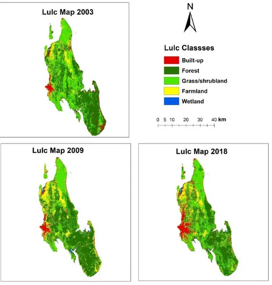
Figure 5. 1: LULC classified maps for the year 2003-2018 ... 27
Figure 5. 2: Land cover maps for 2018 actual (left) and simulated (right) ... 31
Figure 5. 3: Simulated LULC maps for 2027... 33
Figure 5. 4: Comparisons of LULC changes from 2018- 2027 for all three scenarios ... 34
Figure 5. 5: Trends of overall ERI from 2003 - 2027 ... 37
Figure 5. 6: Trend of ERI per district 2003 - 2009 ... 39
1
1. INTRODUCTION
In recent years, the ecological and environmental impacts caused by land transformation have been reported to grow at a very rapid rate and considered to be a major problem around the globe (Qiu, Pan, Zhu, Amable, & Xu, 2019; Shan et al., 2019). These ecological impacts caused by land transformation is connected with the exploitation of natural resources, destruction of biodiversity, as well as disturbing ecosystem structure that offer essential services to mankind including nutrient cycling, pollination, predator control, carbon sequestration and soil fertility (Benton, Solan, Travis, & Sait, 2007).
According to Belay & Mengistu (2019), Africa and Asia are the main areas with the high intensities and dramatic ecological problems caused by LU dynamics. The drivers like over populations, improper controlling of land resources, together with poor economic situations have made these regions be highly adopted with these ecological problems (Wangai, Burkhard, & Müller, 2016). For instance, the studies of Eva et al., (2006), show that between 1975 to 2000, more than 16% of forest cover and 5% of woodlands and grasslands have been destroyed in the African continent. In east Africa alone including Zanzibar, 48% of the tree cover was destroyed in the period of 29 years from 1986-2015 due to the rapid rate of deforestation and expansion of casual agricultural activities (Acheampong, Macgregor, Sloan, & Sayer, 2019). Most of these destructions were attributed to the threatening of an extremely limited number of natural resources, impairing agricultural lands, rising in irregular and unreliable urban areas, as well as increasing in landscape fragility and ecological shock (Winowiecki, Vågen, & Huising, 2014).
In that sense, the appropriate majors in assessing both ecological health together with environmental quality are very essential in analyzing Land cover efficiency (Winowiecki, Vågen, & Huising, 2014). In addition to that, policies to prevent or mitigating ecological impacts of environmental changes are highly needed but however they require robust scientific evidence. This can not only provide significant suggestions for effective solutions to regional ecological problems, but also can promote the useful interaction of socio–economic–ecological development (J. Wang, He, & Lin, 2018).
In dealing with such kind situation, assessing ecological risk conditions in the landscape using land change maps is an important aspect which can be used to quantify the environmental effects of immediate and long-term damage or harm of certain stressors to an ecosystem at a regional scale (X. Zhang, Shi, & Luo, 2013). The concepts of ecological risk assessment (ERA) have begun back to the 1980s as an assessment tool to evaluate the likelihood of the potential adverse
effects of one or more stress factors on ecosystem (USEPA, 1992; Hakanson, 1980; Hunsaker et al., 1990). These techniques can aid an important role in formulating procedures that can help in reducing negative shock on ecosystem destruction as well as ensuring proper management and precise spatial allocation of the natural resources (De Araujo Barbosa, Atkinson, & Dearing, 2015). They can be used in providing spatially explicitly assessment in several important areas include land cover, biodiversity, carbon sequestration, climatic regulation as well as water and soil-related ecosystems (Alizade Govarchin Ghale, Baykara, & Unal, 2019; Fernández-Guisuraga et al., 2019; Xiao et al., 2019).
Ecosystem functioning indicators like landscape ecological risk indices which can be calculated from land cover maps can provide a better estimation on environmental effects as well as long-term damage to ecosystems of a particular region (X. Zhang, Shi, & Luo, 2013). They can also facilitate in maintaining sustainable development in natural resources and ensure the preservation of integrity and stability of ecosystems, which is important for improving ecological security in fragile and intense ecosystems areas (Zang et al., 2017).
Due to their high capability on providing the useful information in understanding ecosystem damage caused by all kinds of hazards, the studies of ecological risk assessment using land change maps have been widely increased in different area around the globe. They have been developed to analyze the temporal-spatial distribution of landscape ecological risk index in watershed area (Jin et al., 2019), identifies the landscape fragmentation level of green spaces as a results of built-up expansion (Tian, Jim, Tao, & Shi, 2011), identification of an ecological network and the most valued lands for protection (McNeeley, Even, Gioia, Knapp, & Beeton, 2017), and among others. In all of these cases, remote sensing techniques in land use land cover changes have been used as a preliminary stage to acquire the land information first before performing further analysis on calculating ecological indices to assess the likelihood of ecosystem collapse of the given landscape.
The ultimate goal in performing ecological risk assessment in any particular study is to generate the relevant planning information so that climatic and other ecological damages can be reduced to a minimum scale (Aurand, 1995). They seek to use historical land information with the influence of remote sensing to provide the scientific foundation for risk management in natural protection and biodiversity conservation, whose importance can serve in both current and future sustainability of natural resources (Xue et al., 2019).
3
Besides all of these ecological risk assessment benefits, and instead of enormous environmental and ecological problems caused by land-use changes, the studies of assessing ecological problems in African are still very narrow (Wangai et al., 2016). According to a review conducted by Wangai et al., (2016) to assess ecosystem services publications in Africa, it was found that the gap related to ecosystem studies in Africa is still huge. This gap is highly influenced with insufficient data as well as heterogeneity of the influencing factors (Wangai et al., 2016).
According to this review, Tanzania including Zanzibar are among those countries with few ecological assessment studies in Africa. The findings in this review have found that, after analyzing all articles accessible online via ISI Web of Science and open access journals, only 8 ecological assessment articles were found to relate with Tanzania case studies for a period of twelve years (2004-2016). Moreover, in the recent assessment that we have done in online journals to review the studies which relate the land-use change and their implications on ecological problems in Zanzibar in the interval of 2000-2019, only 7 articles were found, none of them were employed to access the ecological risk conditions of Zanzibar landscape.
Ecological health condition around Zanzibar landscape is brutally affected by a combination of human and natural pressures (A Staehr, 2018). If not promptly checked, complete extinction of endemic animals or plants together with intense climatic conditions may occur in the near future (A Staehr, 2018).
Therefore, the aim of this study is to assess the current trends and future projection of ecological risk of Zanzibar as consequences of land cover change.
This aim can be achieved by performing the following specific objectives:
Producing land use land cover maps of Zanzibar island for the year 2003, 2009 and 2018; Identify the dynamics of land-use changes in the study area within those selected times; Projecting the land cover changes of Zanzibar island in the next 9 years;
Estimate the ecological risk indices in all cases.
Thus, the outcome of this study may help in informing authorities to understand the ecological processes and land use dynamics of various land cover classes, along with preventing unmanaged growth and haphazard development of informal housing and infrastructure which may result in a gradual deterioration of the environment and a decline in the quality of life and ecosystem services now and for the future generations.
2. LITERATURE REVIEW
2.1. Ecosystem services and their benefits
Ecosystem services have been explained in a number of definitions and classifications (Sannigrahi et al., 2019). The most common definition of ecosystem services ‘are the benefits that people derive from nature’ (Egoh, 2009). According to the Millennium Ecosystem Assessment, ecosystem services are defined as the benefits that people obtain from the ecosystems, and these services can be classified into provisioning (e.g. fiber, fuelwood); supporting (e.g. nutrient cycling, soil retention); cultural (e.g. recreational and cultural benefits); and regulating (e.g. water and climate regulation) services (MA, 2005).
These services play an important role in supporting life and human wellbeing in different aspects (Y. Wang, Li, Zhang, Li, & Zhou, 2018). The world bank report of 2006, estimated that ecosystem services provide support to more than one billion people who live in extreme poverty worldwide (World Bank, 2006). In Africa and most of other developing countries, ecosystem services consumptive output like crop and fish, contribute subsistence livelihoods and play an important role in providing household’s income, thus contributing in poverty reduction and minimizing vulnerability to the negative shock (Egoh, 2009; Langan, Farmer, Rivington, & Smith, 2018; L. Wang et al., 2019).
On the other hand, the products derived from forests including construction timber, fuel-wood, fruits, medicine, and herbs are supporting a large group of communities in raising their national and individual income, thus provide an extensive benefit in the economic situation (Sannigrahi et al., 2019). In South Africa for example, more than 50 species that are derived from various plants have appeared to be used as herbal remedies during pregnancy and childbirth (Egoh, 2009). Similarly, around 40 plant species are used for veterinary purposes, and more than 400 medicinal plant species are considered as a commercialized trade product (Egoh, 2009).
Apart from those economic benefits, ecosystem services provide a wider range of environmental contributions and stand as the main reasons for climatic regulations, water retention, nutrients, and soil cycling, as well as promoting human well-being (MA, 2005). Urban ecosystems including urban greenspace, for example, can significantly contribute to the wellbeing of city dwellers (McPhearson et al., 2016), and they particularly provide a beneficial for disadvantaged communities (Lakes & Kim, 2012). They can also provide a positive impact on climatic regulations by reducing heat islands effect and carbon sequestration as a result of contributing both physical and mental health of the urban population (John, 2015).
5
Alternatively, the coastal ecosystem like mangrove forest, seagrass beds, and coral reefs, provide strong support to hundreds of species of both hard and soft corals and fish as well as sea turtles, crustaceans, and marine mammals (A Staehr, 2018).
2.2. The Current Status of Ecosystem Services
As (MA, 2005) suggested, ecosystem service benefit “is the benefit that humans derive from ecosystems”. But in reverse, human activities have been coined as the main agent for a major loses or destruction of global natural ecosystems (Chi, Zhang, Xie, & Wang, 2019). They cause a major pressure in ecosystem species, by either improper use of natural resources, or due to increasing in demands of ecosystem services in a particular society.
In that sense, the phrase like “ecosystem service loss” is more connected with the costs that must be paid to relieve the impact of ecosystem destruction on human production and earnings (Haden et al., 2019). According to Millennium Ecosystem Assessment report of 2005, there is a massive decline and threatening of ecosystem health which are comprises with the provision of ecosystem services upon which individuals, communities and entire cultures depend (Overpeck et al., 2013; Rowland, 2019). This 2005 MA report had provided an estimation of more than 60% of the ecosystem services which have been assessed across the globe are already being degraded or are used unsustainably with the potential to become more degraded in the first half of this century.
The drivers like the rapid increase in human population, mining activities, subsequent growth in urbanization and informal settlements, together with other threats, place enormous stress on the ecosystem heath and thus impacts their future sustainability (Engel, 2012). Zanzibar and Tanzania for example, have been reported to experience an extensive decline in the state of its environment through loss of natural habitats and biodiversity for more than three decades (A. I. Ali, 2016). Much of these changes are caused by the changes in LULC which are influenced by increase in human population, economic activities and poor management of urban developments (NEMC, 2006).
Alternatively, the 2018 WWF’s living Planet report, provide an estimation of up to 50% of the global freshwater and wetland habitats which have already been lost in the past 30 years since 1970 due to various human activities and climatic variation (World Wide Fund For Nature (WWF), 2018). These freshwater and wetland habitats are more essential in maintaining ecological processes, as well as providing an appropriate water flows within an entire water catchment (Paul, 2013). Losing or destructing these habitats, would affect the environmental flows including reducing the volume, timing and even the quality of water flows which are very
essential for the survival of downstream habitats and species within those areas (Paul, 2013).
In case of forest ecosystems, which appear to be the most fundamental sources of services and global biodiversity, their ability to maintain their future sustainability is potentially threatened. The recent report of Food and Agriculture Organization, provide an estimation of about five million hectare per year of global forest which have already been lost between 2005 and 2015 (FAO, 2018). This estimation is very worse for the future development of biodiversity and ecosystem sustainability, as well as threat corresponding to the feedback on climatic system and food security (Garzuglia, 2018). Without proper plan and management, the status of ecosystem services will continue to face unprecedented stress and pressure, that could result in their degradation and conversion, thereby affecting their sustainability in both current and future generations.
2.3. The Role of Remote Sensing on Land use and Land Cover Change
Remote sensing is the science and to some extent, the art of acquiring information about the Earth’s surface without actually being in contact with it (Paul, 2013). In combination with GIS, Remote Sensing (RS) provide a better opportunity in studying and analyzing the various form of the earth's information (Paul, 2013). It provides rooms to view the earth phenomenon from the space, which enables the comprehension of the cumulative influence of human activities on the earth's surface's natural state.
One of the major applications of remote sensing techniques is the classification of remotely sensed data of multi-temporal images. These techniques have been considered as an ultimate root for various analysis and applications in the field of remote sensing (Müllerová, Pergl, & Pyšek, 2013). The fundamental objective of remote sensing image classification is to divide the remotely sensed image into a number of classes (pixel group) in order to effectively examine and asses what changes have been occurred in each of those groups (J. Xu, Feng, Zhao, Sun, & Zhu, 2019).
However, the classification process of remotely sensed images is sometime considered to be the most complex task influenced by various factors such as availability of high-quality images, ancillary data, proper classification procedure, and analytical ability of the researcher (Gao & Xu, 2015) . In most cases, it appears to be much harder to identify which is the best classifier to be used in a particular study due to either the lack of proper guidelines in selecting the algorithm or even the lack of availability of appropriate classification algorithms to a particular band (Gao & Xu, 2015). In that sense, many researchers have made a great effort in proposing the most effective classification methods to improve classification accuracy and as well as their results.
7
The most popular remote sensing classification methods proposed in different studies are supervised, and unsupervised classification. In supervised classification, the image pixels are classified by selecting representative samples for each land cover class (Training Sites or Areas) and then the classification algorithm applies these samples to the entire image (Bhattacharya, Carr, & Pal, 2016). This process is done in three major steps including selecting training areas, generate the signature file and classify the image. In another case, in unsupervised classification the images are classified only by grouping the pixels into clusters based on their properties first, and then the classification of each cluster with land cover classes are done. In general, this classification method is considered as the most basic technique, since there is no need of training samples to classify the image. It is a simple way to classify the image with only two major steps including generating clusters and assigning classes (Bhattacharya et al., 2016).
All of these classification methods can be further grouped in either statistical methods, decision trees, artificial neural networks, and other artificial intelligence algorithms (Xie, Li, Xiao, & Peng, 2016). Statistical methods such as maximum likelihood classifier and Bayesian classifier works in an assumption that the members of each class in each band follow a normal distribution in the feature space and calculates the probability that a given pixel belongs to a specific class. In this particular method, the classification accuracy decreases as the dimension of feature decreases (Xie et al., 2016).
The decision tree methods like random forest classifier make no assumptions concerning the distribution of the input features and therefore they are robust and effective methods in managing nonlinear relationships among the class member (J. Xu et al., 2019). However, the effectiveness of the decision tree methods is highly influenced by the size of the feature space and thus are not appropriate methods for data with a high dimension of feature space (J. Xu et al., 2019).
In the case of artificial neural networks (ANN) methods prove a powerful performance with a higher dimensional feature space compared to statistical classification methods because they are distribution-free (J. Xu et al., 2019). However, the most difficultness of using ANN models is its demands to requires a significant amount of training data and a considerable number of iterative training procedures to ensure that the models are trained successfully. Alternatively, the computation of ANN algorithms can be extraordinarily complex (J. Xu et al., 2019).
2.4. Future Provisions of Ecological Monitoring through Land Change Modeler
Spatial and dynamic changes in LULC of the earth’s surface have a major influence on the destruction and future provision of ecosystem sustainability for both landscape structure and fragmentation of green space (Tian, Jim, Tao, & Shi, 2011). These dynamic changes in LULC can result in an increase in the level of land abandonment, starvation or even migration out of the affected region (Y. Wang et al., 2018). In that kind of situation, understanding the dynamics and future land cover trends has to be considered as a major component in approval strategies for both the planning and implementation of appropriate tools in conserving the degraded land.
A number of computation algorithms for monitoring and predicting future land cover changes have been widely increased in recent years. The models like Markov chain (MC) (Al-sharif & Pradhan, 2014), artificial neural network (Pijanowski, Brown, Shellito, & Manik, 2001), cellular automata (Clarke & Gaydos, 1998), cellular Automata-Markov model (Arsanjani, Kainz, & Mousivand, 2011), binary logistic regression (Arsanjani, Helbich, Kainz, & Boloorani, 2012), and similarity weighted instance-based machine learning algorithm (Sangermano, Eastman, & Zhu, 2010) are among the common used models for the future prediction and simulation of changes in land cover.
Land Change Modeler (LCM) for example, was found to be one among the effective modeling tool which incorporates CA-Markov chain based on a neural network to predict future land-use change (Eastman, 2006). This CA-Markov chain models incorporated in LCM are fairly simple and much powerful in modeling the complex process and changes in land use for planning purposes (Eastman, 2006). It models the future land cover changes by making an assumption that, the probability of system being in a certain time can only be determined if its previous state is known with the assumption that rates of change observed during the calibration period (T1 to T2), will remain the same during the simulation period (T2 to T3).
LCM does also provides the tools that can simulate the future land-use changes and patterns and allowing testing of alternative planning scenarios. Simulating future land cover change under what called scenarios, can provide a better understanding of various planning alternatives, stimulating policy discussions between environmental and development goals, and therefore helping the responsible authorities in designing the new policies and procedures that create incentives for ecological conservation (McKenzie, E., Rosenthal, A., Bernhardt, J., Girvetz, E., Kovacs, K., Olwero, N. and Toft, 2012).
9
3.
STUDY AREA
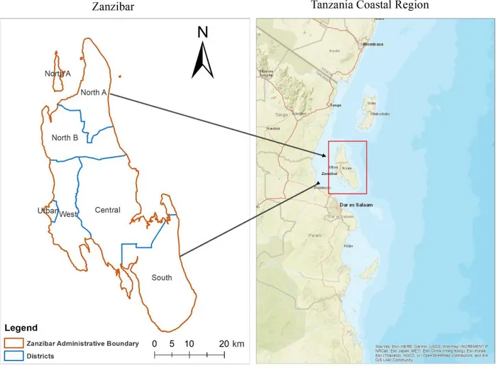
This study was conducted in Zanzibar (Figure 3.1), the small coastal island of about 2,461 km² in total, located at 39° 05’ E to 39° 55’ E and 4° 45’S to 6° 30’S Western Indian Ocean, in which tourism and agricultural activities are the major economic sectors contributing about 28% and 40% of its GDP respectively (WB, 2019).
Zanzibar is a part of the United Republic of Tanzania, and consists of two main islands which are Unguja and Pemba and with almost 50 other small islets (Myers, 2010; RGZ, 2008). These two islands are located 40 km off the mainland coast of East Africa in the Indian Ocean (Myers, 2010). The two main islands are 50 km apart and are separated by the 700 meter deep Pemba channel. However, the current study uses the term Zanzibar referring to the island of Unguja as most of the people live in this island (Unguja), and because of Zanzibar city located in it (A Staehr, 2018).
According to 2018 National Bureau of Statistics (NBS) census report, the overall population of Zanzibar island (include Pemba) is about 1,348,776 people and its annual growth increase in a very rapid rate. In the recent years, the population growth rate of Zanzibar has been reported to grow at a rate of 3.4 % annually (NBS, 2018). Natural population growth is considered as the main agent for this high rapid rate, but other factors including growing of tourism industry and economic influence has also attracted a significant number of migrants from Tanzania mainland and other parts of East Africa, making this island to be one among the highly populated islands in the world.
Zanzibar has a tropical climate with four distinct seasons. “Kaskazi” (the hot season, which is between December and February and associated with either little or no rains), “Masika” which is the long rainy season from March – May, “Kipupwe” (the cold season, with strong winds between June and September), and “Vuli” which is very short rainy season from October – December. The annual rainfall of island is ranging from 1600 mm for Unguja and 1900 mm for Pemba respectively, and the air temperatures is ranging between 29 and 32ºC on average. Zanzibar island was originally forested, but pressures like population increase, human habitation and climate change and variability have resulted in widespread clearing of the forest and vegetation cover (M. Kukkonen & Käyhkö, 2014).
Figure 3. 1: Study Area-Zanzibar
The land cover patterns around Zanzibar island are generally distributed under two different soil classes, namely the deep soil and the coral rag areas. The deep soil areas are mainly attributed by permanent cultivation and forest, while the later coral rag are characterized by cultivation and consequent scrublands (RGZ, 2008). However, all of these two soil classes are not stable in terms of its land cover and biotope characteristics. The hilly deep soil areas are reported to be more vulnerable to soil erosion, highly land use demands and simultaneously facing population pressure, which all of these influences the rapid and constant changes in land cover patterns and natural resource (M. Kukkonen & Käyhkö, 2014; Myers, 2010). Alternatively, shifting cultivation characterized in coral rag areas create a constant element of changes, which under the pressure of diminishing area due to commercial and conservation land use may leads towards deterioration of ecosystems and valuable natural resources (Myers, 2010).
11
4. DATA AND METHODS
4.1.
Description of the data
Data from different sources were used to achieve the objectives of this study. At very first stages, the remote sensed satellite images of Zanzibar island (Table 4. 1) at different time were obtained from USGS website (www.earthexplorer.usgs.gov/), and then compared based on their different temporal phenomenon. In that sense, three multispectral Landsat images of the year 2003, 2009 and 2018 with spatial resolution of 30 m were downloaded from USGS website (Table 4.1).
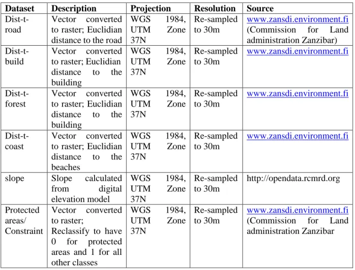
Ancillary data representing biophysical properties that were considered to influence land use changes were also applied in this analysis. These ancillary data were obtained by first downloading their original shape files including Zanzibar road, protected forest, buildings and villages as well as coastal region from (www.zansdi.environment.fi ). By means of digital elevation model (DEM) which was obtained from ( http://opendata.rcmrd.org ), we calculate the distance for each of these variables to create the biophysical properties of distance to the road, distance to the buildings, distance to the coast, distance to the forest and slope (Table 4.2).
Protected areas including protected forest, governmental agricultural field, as well as open and restricted zones were also used to represent the constraints of land cover changes in the study region. These protected areas data were obtained by reclassifying the 2012 Zanzibar LULC map which was obtained from Zanzibar commission for land (COLA) to create a Boolean map of 0 for protected areas and 1 for all other classes (Figure 4.3).
Dataset Description Projection Resolution Source Landsat 7, ETM+ Raw = 064, path = 166, Date: 14/01/2003 WGS 1984, UTM Zone 37N 30 m www.earthexplorer.usgs.gov/ Landsat 5 TM Raw = 064, path = 166, Date: 1/07/2009 WGS 1984, UTM Zone 37N 30 m www.earthexplorer.usgs.gov/ Landsat 7, ETM+ Raw = 064, path = 166, Date: 18/07/2018 WGS 1984, UTM Zone 37N 30 m www.earthexplorer.usgs.gov/ Digital Elevation Model (DEM) SRTM Clipped from Tanzania Dem WGS 1984, UTM Zone 37N STRM 30 m http://opendata.rcmrd.org
Table 4.1: Satellite Data
4.1.1. External variables
In modeling LULC change for a specific area, the variables influencing or controlling the land cover change on that area should be properly used as independent variables, and the LU maps should be used as dependent variables. The inclusion of independent variables in land change modeling is very essential since these variables ensure the future land cover maps are always predicted with existing patterns and drivers of changes in that region (Bulley, & Fürst, 2017).
In this study, the selection of independent variables was based on reviews related to similar models, researches conducted in other developing countries as well as the local circumstances of Zanzibar island. In that sense, the variables slope, distance to the road, distance to the forest, distance to buildings, distance to the coast and protected areas were all selected as independent variables to simulate the future land cover change for Zanzibar city.
The variable “slope “was chosen to represent the biophysical conditions of the study area. According to (Liu, 2009; Arsanjani et al., 2013), the flat topography has much influence on land cover changes than rugged topography, and this theory has already been used in many similar models with positive results (Zhao et al., 2014).
“Distance to the roads” and “distance to the forest” were all connected to economic circumstances. The chosen of distance to the forest in economic factors is connected with the fact that in Zanzibar, the customs of converting forested land into either built-up areas or farmland is one of the major reason of land-use dynamics, and this is highly caused by the economic situation of Zanzibar population (M. Kukkonen & Käyhkö, 2014). This variable is also related to local
13
spatial policies forbidding any constructions or development activities in protected forest (M. Kukkonen & Käyhkö, 2014).
We regard “distance to the coast” and “distance to buildings” to be connected in the social factors. In this case, the variable “distance to the coast” confirms the global trend towards higher quantities of land-use changes in coastal regions (Ebadati, 2018). And for the second variable “distance to the buildings” express the local social and planning conditions of Zanzibar, in which the houses are built relatively close to each other due to subdivisions of small landholdings. In other case, this phenomenon is also related to spatial interactions, provided that the land-use changes are highly attracted by similar changes in their neighboring areas (M. O. Kukkonen et al., 2018; ToblersFirstLawofGeography, n.d.).
And in the case of the remaining variable “protected areas”, it has been used to represent the local spatial policies that have either obstructed or indirectly stimulated land-use dynamics (M. O. Kukkonen et al., 2018).
Dataset Description Projection Resolution Source
Dist-t-road
Vector converted to raster; Euclidian distance to the road
WGS 1984, UTM Zone 37N Re-sampled to 30m www.zansdi.environment.fi (Commission for Land administration Zanzibar) Dist-t-build Vector converted to raster; Euclidian distance to the building WGS 1984, UTM Zone 37N Re-sampled to 30m www.zansdi.environment.fi Dist-t-forest Vector converted to raster; Euclidian distance to the building WGS 1984, UTM Zone 37N Re-sampled to 30m www.zansdi.environment.fi Dist-t-coast Vector converted to raster; Euclidian distance to the beaches WGS 1984, UTM Zone 37N Re-sampled to 30m www.zansdi.environment.fi
slope Slope calculated
from digital elevation model WGS 1984, UTM Zone 37N Re-sampled to 30m http://opendata.rcmrd.org Protected areas/ Constraint Vector converted to raster; Reclassify to have 0 for protected areas and 1 for all other classes WGS 1984, UTM Zone 37N Re-sampled to 30m www.zansdi.environment.fi (Commission for Land administration Zanzibar
4.2.
Methods
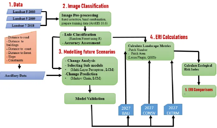
The overall methodology for this study was carried out into three major steps (Figure 4.1). First, the land use land cover classification was performed using random forest classifier to generate three LULC maps of 2003, 2009 and 2018. Next the land cover maps for the future scenarios were modeled using land change modeler of the TerrSet 18.3 software. And finally, the ecological risk indices for each map and each district of Zanzibar were calculated by first computing the landscape metrics using LECOS plugin in QGIS 3.8, followed by applying the formulas from various literatures for ERI assessment (Xue et al., 2019; F. Zhang et al., 2018; X. Zhang et al., 2013).
4.2.1. Image classification
Pre-processing of all three satellite images (2003, 2009 and 2018), Zanzibar administrative boundary, together with all ancillary data Shapefiles, was performed by using ArcGIS 10.6. All datasets were projected to WGS 1984, UTM Zone 37S coordinate system, followed by band combination, clipping of the study region, and resampling of each one of them to appear in the same spatial resolution of 30 m.
Training Samples Shapefile of five classes including built-up, grassland, forest, wetland and farmland were generated by digitizing each of the satellite images. With these generated five land
15
use classes training samples, the random forest classifier algorithm was employed in RStudio v3.5.3 (R Core Team, 2018) to produce land use maps for each study year.
Random forest algorithm is a supervised machine learning algorithm that generates estimators which fits a number of decision trees on various subsets of the training data set. The algorithm creates decision trees on data samples and then gets the prediction from each of them and finally selects the best solution by means of voting (Gislason, Benediktsson, & Sveinsson, 2006). Random forest classifier is mainly used for classification problems, since it provides better results due to its capability of reduces over-fitting problem by averaging the result (Gislason et al., 2006).
In this case, the composite image for each year and their corresponding training samples were separately imported in the model algorithm to produce LULC maps for each year.
The produced LULC maps were then used to calculate the percentage changes for each LULC classes in the study region via a formula indicated below.
𝐿𝐶𝐸 =𝐿𝐶𝑓 − 𝐿𝐶𝑖
𝐿𝐶𝑓 × 100% Where:
LCE: Land cover change
LCf: land cover area in final map LCi: Land cover area in initial map
4.2.2. Accuracy assessment
The classifications result for each of the classified image were validated through an accuracy assessment process using data points from classified satellite images, and then verified with the ground truth points collected from Google Earth. The ground truth process was undertaken to ensure that the observation appears in classified images refers to what is actually on the ground by correlating with the corresponding features on the image scene (Tilahun, 2015). About 200 ground truth points were collected in Google Earth for each year of the classified images. These ground truth points were then compared with the pixels of the classified images using ArcGIS 10.6. Finally, the confusion matrix for each of the classified image was generated and used to calculate the overall accuracy, producer’s accuracy, user’s accuracy, as well as the kappa coefficient.
4.3.
Descriptions of the chosen scenarios
4.3.1. Business as usual (2027BAU)
In this scenario, the 2027 map was modelled based on the existing land use policies, plans and regulations in Zanzibar city. Therefore, the protected area constraint (Figure 4.3 left) that was designed to ensure that no land use change will happen in all of the existing protected and restricted zones were employed in this scenario. The focus here was to have a clear understanding of what would have to happen in the future land cover change if nothing regarding to the land use policies and restrictions would be changed in the study region.
4.3.2. Conservation scenario (2027CONSV)
In 2027 conservation scenario, the 2027 land use map was modelled by employing constraint that make restrictions of no land use change in all substantial agricultural areas, the high coral forest as well as in all restricted zones (Figure 4.3 right). The idea here was to conserve forest and substantial agricultural areas from being exploited by informal settlement and casual farming activities which are considered to be the main agents for unreliable land cover changes in Zanzibar (M. O. Kukkonen et al., 2018). This scenario is also related to local spatial policy of Zanzibar in forbidding construction of buildings in open agricultural areas and restricted forest (Kukkonen et al., 2018; RGZ, 2008).
4.3.3. Extreme scenario (2027EXTM)
In extreme scenario, we modelled 2027 land cover map without employing any constraint and restriction policy, such that the land use changes are allowed in any area within the study region. The reason behind, is to analyze what would happen in the future land cover changes if we ignore any protection majors and allow land use changes to occur anywhere in the study region. This is very important scenario in Zanzibar, even more than business as usual. It is because in Zanzibar the development and construction of the buildings in random way and without following restrictions is one among the major common problem facing the urban planning (M. H. Ali & Sulaiman, 2006). And therefore, it is really important to inform authorities on the future consequences of this defective habits such that the authority can take a quick response.
17
4.4.
Preparation of external (independent) variables
Before applying land change modeler (LCM) to model the future scenarios of land cover change, the external variables (both constraints and factors) that was considered to influence or restrict the land cover changes in the study region were prepared.
Constraints are variables that restrict or limit use changes in specific areas based on land-use policies, rules, and regulations. These variables are expressed in form of a Boolean map such that those areas which are restricted from land-use changes are being assigned a value of 0 (unsuitable), while those areas in which land-use changes are permitted, the value of 1are assigned (suitable) (Eastman, 2006).
In another case, factors are the variables that influence the dynamic changes of the land cover depending on the appropriate activity under consideration. These variables are not reduced to simple Boolean constraints, and therefore, most commonly measured on a continuous scale (Eastman, 2006).
4.4.1. Factors Preparations
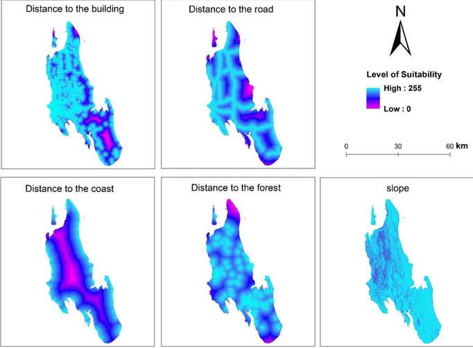
As mentioned earlier, the variables distance to the road, distance to the forest, distance to the buildings, distance to the coastline as well as the slope were chosen as external factors influencing the land use change in this study.
These variables were first prepared by calculating Euclidean distance for each one of them in Arc-GIS 10.6. Next, their resultant distance maps were imported to IDRISI Selva v17.02 and standardized them in a continuous scale of suitability (Figure 4.2).
Rescaling and standardizes the factors in a continuous scale of suitability, help in enhancing the performance and speed of Multi Criteria Evaluation (MCE) (Hirscher, Schweizer, Weller, & Kronmüller, 1996). And because, the Multi Criteria Evaluation (MCE) module in IDRISI has been optimized for speed using a 0-255-byte level of standardization (Eastman, 2006), then the fuzzy standardization module in the scale of 0-255 with three different functions were used to rescale each of these variables.
Araya & Cabral (2010), have already described these three functions in designing the criteria’s for the factors to be used in decision rule. These functions include sigmoid, J-shaped and linear functions with some adjustable settings. And therefore, based on these three opinions, all factors
in this study were standardized and categorized.
In case of the distance to the forest, distance to the buildings and distance to the coastline, linear monotonically decreasing function with control point a = 0, and d = 12241, 6467, 12802 respectively were used, implying that suitability decreasing with distance. In this context, the parameter a implies the closer distance from variable, while b represent the highest distances of each variable obtained from the distance maps calculated in ArcGIS.
Since in Zanzibar there is a policy which restricting any constructions or development activities within 20 m buffer from the road networks, a linear symmetric function with control point a = 0, b = 20, c = 20 and d = 10607 was applied for the distance to the road. This means that, the areas within 20 m are not suitable for LU changes. However, areas between 20 m and 10607 m the suitability is decreasing with the highest suitability being near to a 20 m.
And finally in case of slope variable, the sigmoidal monotonically decreasing function with control point a = 0, and c = 17 were used. This is because, for the slope purposes in Zanzibar, all areas above 17% of slope, are considered to be less suitable or invulnerable for LU changes.
19
4.4.2. Constraints
Two constraint maps were created in this study, one for business as usual, and the rest for conservation scenario (Figure 4.3). The constraint for business as usual was created by reclassifying 2012 LULC map of Zanzibar island which was obtained from Zanzibar commission for land (COLA) and assign the value of 0 for those protected areas (to exclude them in LULC changes), and 1 for all other areas (suitable and more vulnerable for LULC changes). The constraint map for conservation scenario was created by assigning the value of 0 for those protected areas, high coral forest cover, as well as all subsidence agricultural sites. The focus was to exclude all of these areas in future land cover changes. However, in all other areas, the value of 1 was assigned implying that they are allowed for future LULC changes.
4.5.
Modelling Future Scenarios with LCM
We model land cover for 2027 in three different scenarios based on constraint maps. With three selected factors and protected area constraints (Figure 4.3 right) the land cover for business as usual was simulated. The land cover for the conservation scenario was modeled by combining the three selected factors and the conservation constraint (Figure 4.3 left). And in case of extreme scenario, the 2027 land cover was modeled without employing any constraint, only the three selected external factors were used.
In this stage of modelling the future scenarios, three steps of analysis including change analysis, transition potential, and change prediction were performed.
4.5.1. Change Analysis
The first step of modelling land cover maps with land change modeler is to perform change analysis stage in which the historical land cover maps should be used as input images to examine the amount of gain and losses, net change, and contributor to change from each category of land cover classes within the specified time period.
In this study, the change analysis process was performed in two different steps. First, the maps of 2003 and 2009 were used as an input images to derive all historical information described above including the maps of gains and losses, contributions to net change and transitions of land cover classes, as well as the spatial trend of land-use classes. The focus in this first phase was to use these historical pieces of information to simulate the land cover map for the year 2018 so that it can be compared with the actual classified map of 2018 to estimate the predictive ability of the model (model validation).
And in the second phase, the change analysis process was performed by employing the land use maps of 2009 and 2018 as input images. In this case, the idea was to acquire the same information described in step one above to predict the land use maps for the 2027 scenarios.
21
4.5.2. Transition potential
After finishing the first step of change analysis, the next step was to test the explanatory power for each external variable, as well as selecting transition sub-models that are relevant in the prediction of the future scenarios.
Therefore, in this stage, first, the Cramer’s power of all external variables were tested to identify all variables with a potential explanatory power. These Cramer’s power are ranging from 0 – 1, in which the variables with at least 0.15 Cramer’s value are considered to be potential in land use changes, whereas those having value from 0.4 onward are much potential (Eastman, 2006). The results of Cramer’s power for each tested variable are illustrated in (Table 4.1) below.
Explanatory Variable Overall Cramer’s V value
Distance to buildings 0.2852
Distance to road 0.1836
Distance to the coastal area 0.1653 Distance to the forest 0.1354
Slope 0.0725
Restricted areas 0.1932
Table 4. 3: Cramer's power for external variables
Due to the lower Cramer’s value, negative influence on the modelling results, as well as less literatures information regarding to Slope issues in Zanzibar, this variable was excluded in analysis.
In the same sense, the variable distance to the forest was also removed from the analysis due its lower Cramer’s power and its negative influence on the analysis accuracy.
Therefore, only three external factors including distance to the building, distance to the road and distance to the coast, and one constraint map for each scenario (except for extreme scenario, where constraints were not employed) were used in this analysis.
The next step was to combine all selected variables (factors and constraint) together with transitions sub-models between 2003 and 2009 and employ Multi-Layer Perceptron (MLP) to generate transition potential for 2018 land cover map prediction.
Multi-Layer perceptron (MLP) is a feedforward artificial neural network (ANN) composed with one or multiple layers including input, output and hidden layers between input and output layer. The term feed-forward method implying that the data flows in one direction from input to output.
The main algorithm of this model is computing the linear output from nonlinear inputs according to the weights by using a nonlinear activation function (Gardner & Dorling, 1998).
MLP employs a supervised learning technique called backpropagation for training. The back-propagation algorithm composed of two steps which are forward pass and backward pass. In the forward pass, activation transmits from input to output layer which means that the signal flow moves from the input layer through the hidden layers to the output layer. While in backward pass errors propagated from output to hidden layer (Gardner & Dorling, 1998).
To model land-use transitions in LCM, either Logistic Regression, SimWeight or MLP neural network can be applied. However, in this study, the MLP neural network was applied because of its capability of running multiple transitions of up to 9 per sub-model as well as explanatory variables at once (Eastman, 2006).
To achieve the better accuracy on the results of Multi-Layer Perceptron only major land cover transitions together with only the driver’s variables with higher Cramer’s power should be included in the transition sub-model (Eastman, 2006).
Based on this principle, together with the information from literatures regarding on study region, only six major transitions including grassland to built-up, forest to built-up, grassland to farmland, forest to grassland, forest to farmland and farmland to grassland were selected in this study. Together with four selected variables, a Multi-layer perceptron was employed with an accuracy of 68.4% to generate the transition potentials (Figure 4.5) that were then used by Markov chain method to predict the Land use map for the year 2018.
23
Figure 4. 4: Transition Potential 2003 - 2009
4.5.3. Change prediction
The third stage in modeling future scenarios was to perform change prediction to a future specified date for the allocation of land cover changes. In this stage, the default procedure in LCM (Markov Chain analysis) was applied to determine the amount of changes at a date of 2018 based on historical land cover maps of 2003-2009.
Here, the algorithm determines exactly how much land would be expected to transition from the later date (2009) to the prediction date (2018) based on a projection of the transition potentials maps that was generated and then creates a transition probabilities file (Eastman, 2006).
With this transition probabilities file, two predictors maps which are soft prediction map and a hard prediction map were generated. While a soft prediction map is a continuous mapping of vulnerability to change which provides an indication of the degree to which the areas have the right conditions to precipitate change in 2018, a hard prediction map is an actual projected map of 2018, in which each pixel is assigned one land cover class; the class that it is most likely to become (Eastman, 2006).
4.5.4. Model validation
To ensure the predictive ability and performance of the model. Model validation and calibration must be performed before starting the prediction of LU changes for the specified date. Performing validation of the model is a very important step because the efficiency and usability of the model are always depending on the output of the validation (van Vliet et al., 2016).
Since several studies have already proposed the usage of the confusion matrix (Congalton, 2001) in assessing the accuracy and performance of the model, we also compute the confusion matrix by performing cross-tabulation to compare the actual and simulated maps of 2018. The confusion matrix which was generated after performing cross-tabulation was then used to calculate the overall accuracy, user accuracies, producer accuracies, and kappa coefficient.
In addition to that, two other kappa coefficients were also computed to gain more information on the performance of the model. The other two kappa coefficients are Khisto and Klocation. According to Serna, (2011), Khisto is used to measure the similarities in the number of cells between simulated and reference maps. In other words, this kappa is responsible for measuring quantitative similarity between two compared maps. In another case, Klocation is used to measure the similarities in the spatial distribution of classes but does not differentiate between classes that are close or distant and it is independent of the total number of cells per class (Serna, 2011).
25
4.6. Calculation of Ecological risk indices
The final step of our analysis was to compute ecological risk indices for each LULC map, as well as for each district of Zanzibar island and then comparing their results. This stage was done in two major steps. First the landscape metrics (patch number and patch area) for each LULC maps was calculated using LECOS plugin in QGIS 3.8, and then the formulas described in section 4.6.1 below were used to calculate ecological risk indices for each map.
Ecological Risk index (ERI)
Provide an indicators of the negative environmental impacts that may occur or are occurring due to one or more external factors (USEPA, 1992; Hakanson, 1980; Hunsaker et al., 1990, X. Zhang et al., 2013) . Mathematically: 𝐸𝑅𝐼 = ∑𝐴𝑘𝑖 𝐴𝑘 𝑛 𝑖=1 𝑅𝑖 Where:
ERI: The ecological risk index of the risk area Ak: is the total area of kth region
Aki = is the ith landscape area/class area
Ri: is the ith landscape/class loss index which can be calculated through formula below.
𝑅𝑖 = 𝐹𝑖 ∗ 𝑆𝑖
Where: Fi, is the ecological fragility index which is referred as the ability of a landscape to resist the human disturbance.
According to Zhang et al (2013), and the knowledge of our study region, the Fi value of 5 for built up, 4 for water body, 3 for grass land, 2 for farm land and 1 for forest were used in this study. Additionally, for an effective result, these values were normalized before directly being used in calculations of ecological risk index.
Si is the landscape disturbance degree index of ith landscape (Jin et al., 2019), which can also be calculated via a formula.
Where:
Ci: Land scape fragmentation, it reflects the changes in landscape structure and ecological process, 𝐶𝑖 = 𝑛𝑖
𝐴𝑘𝑖
Ni: Land scape isolation, refers to the degree of separation of patches in a given landscape type,
𝑁𝑖 = 𝐴𝑘
2𝐴𝑘𝑖√
𝑛𝑖 𝐴𝑘
Di: Landscape dominance index, describe the dominance of patches in a given landscape,
𝐷𝑖 =𝑄𝑖 + 𝑀𝑖 + 𝐿𝑖 3
ni: Is patch number of ith land scape, Qi: Ratio of the cell with ith patch and total cell, Mi: Ratio of the number of ith patches to total patches and Li: Ratio of ith patch area to the total area. And a, b and c: represent the weight of Ci, Ni and Di respectively where a + b + c = 1 (Zhang et al, 2013).
27
5. RESULTS
5.1. LULC changes 2003 - 2018
Figure 5.1 below illustrate the LULC classified maps for the year 2003-2009. As it can be seen, the visual interpretation of the classified images explores extensive changes in various land cover classes in the study region especially the rapid expansion of built up area as well as decrease in forest cover. The high increase in built-up area is highly exposed in eastern zone of the study region which are near to the urban center of Zanzibar island.
5.2. Accuracy assessment
Accuracy assessment for each land use map was performed in order to find classification errors and make the produced land cover maps become reliable and easily interpretable by users. Kappa coefficient, overall accuracy, user accuracy as well as producer accuracy were all calculated and the assessment results were summarized in (table 5.1, 5.2 and 5.3) below.
The assessment results for each of the produced land cover maps provide an overall accuracy ranging from 74% - 78%, and overall kappa coefficient which is ranging from 0.68 – 0.71. On the other hand, the users and producer’s accuracies computed for each of the classified maps were all above 65%. These results indicating that the classified images have met a good level of accuracy and thus they are satisfying for the study analysis.
In all of the three classified images, the wetland has shown a high user’s accuracy (80% - 89%) compared with other land use classes. This implied that the majority of their pixels were correctly classified in their respective classes. However, in each classified image either farmland, grassland or forest cover provides a minimum users or producers accuracy (63%-80%).
The maximum user’s accuracies provided by the wetland can be justified by their distinctive characteristics in comparisons with other LU classes. This characteristic makes them easily being discriminated by classification algorithms against other land use classes during the classification process. However, on another side, the lowest users and producer’s accuracies for farmland, grassland and forest cover can be explained by their spectral property similarities among them (Melville, Lucieer, & Aryal, 2018).
overall accuracy 76%
kappa 0.69
LULC classes Built-up Forest grassland farmland Wetland Total User accuracy
Buildup 32 0 5 3 2 42 76% Forest 2 37 6 0 1 46 80% Grassland 1 6 36 6 1 50 72% Farmland 5 5 3 31 0 44 70% Wetland 0 2 0 0 16 18 88% Total 40 50 50 40 20 200 Producers accuracy 80% 74% 72% 77% 80%
29
Overall
accuracy 78%
kappa 0.71
LULC classes Built-up Forest grassland farmland Wetland Total User accuracy
Buildup 34 2 2 3 3 44 77% Forest 0 41 9 0 1 51 80% Grassland 1 3 35 8 0 47 74% farmland 5 3 3 29 0 40 73% Wetland 0 1 1 0 16 18 89% Total 40 50 50 40 20 200 Producers accuracy 85% 82.00% 70% 72% 80%
Table 5. 2: Confusion matrix for LULC map of the year 2009
Overall accuracy 75%
kappa 0.68
LULC classes Built-up Forest grassland farmland Wetland Total User accuracy
Buildup 33 1 1 4 2 41 80% Forest 1 39 6 3 0 49 79% Grassland 1 6 34 6 1 48 70% farmland 5 1 9 26 0 41 63% Wetland 0 3 0 1 17 21 80% Total 40 50 50 40 20 200 Producers accuracy 82% 78.00% 68% 65% 85%
5.3. LULC changes 2003 - 2018
The statistical results corresponding to LULC change in the study areas (Table 5.4) indicating that, there is an extensive increase in the built-up area as equivalent to the decrease in forest cover. The built-up area of Zanzibar island has been expanding from 4132.44 Hectare in the year 2003 to 7201.35 Hectare in 2018. These areal changes in the built-up area make up of 42.6% increase in construction land for only 15 years’ (2003-2018) period (2.84% increase annually).
The Farmland/agricultural land has also shown a progressive expansion within these 15 years of the study, in which 31.7% (2.1% annually) of agricultural land were increased.
For the forest cover and wetland, the trends on their land cover changes have shown a continuously decreasing, in which 15.8% of forest cover (1.05% annually) and 24.6% of wetland (1.64% annually) were disappeared.
However, in the case of grassland, the trend in its LULC changes does not show a smooth variation. This is because, in the first 6 years (2003-2009), the grass cover of the study area has been decreased by 4.5%, followed by increasing of 7.48% for the next 9 years (2009 – 2018).
LULC classes Area (ha) (2003) Area (ha) (2009) Area ( (2018) % changes (2003-2009) % changes (2009-2018) % changes (2003-2018) Built-up 4132.44 5081.94 7201.35 18.68 29.43 42.62 Forest 73329.39 69460.56 61692.03 -5.28 -11.18 -15.87 Farmland 22171.77 27669.15 29206.17 24.79 5.26 31.73 Grassland 56569.41 54107.73 58484.43 -4.55 7.48 3.27 Wetland 1925.55 1809.18 1544.58 -6.43 -17.13 -24.66
Table 5. 4: LULC areal statistics from 2003 -2018
This rapid LULC changes of several land cover classes within the study region could be attributed by the improper way of managing the land including the high rate of informal settlement, casual farming methods as well as the higher level of deforestation activities in Zanzibar (M. O. Kukkonen et al., 2018).
31
5.4. Land Cover Change for future Scenarios
5.4.1. Model validation results
As explained in section 4.5.4 above, the model validation in this study was performed by comparing the simulated map and actual map of 2018 (Figure 5.4) by using cross tabulation and validation module to compute the overall accuracy, user accuracies, producer’s accuracies, kappa coefficient as well as two other kappa coefficients including Khisto and Klocation.
Figure 5. 2: Land cover maps for 2018 actual (left) and simulated (right)
The cross-tabulation results obtained after comparing the actual and simulated map of 2018 are shown in (Table 5.5) and as it can be seen, the overall accuracy of the model is 75% and with a kappa coefficient of 0.65. In almost all classes the user and producer’s accuracies were all above 65% which indicate a good level of accuracy. However, the user and producer accuracies for grassland and farmland are seems to be a little bit lower (58% and 63% respectively). These lower producers and user’s accuracies for these two classes can be explained by their spectral property similarities among them (Melville, Lucieer, & Aryal, 2018).