Modelling evapotranspiration of soilless cut roses "Red Naomi" based on climatic and crop predictors

(1)

Modelling evapotranspiration of soilless cut roses

‘Red Naomi’ based on climatic and crop predictors

Patricia Malva Costa

1

_{, Isabel Pôças}

1,2,3,4

_{, Mário Cunha}

1,3,4

_*

1_{Faculdade de Ciências da Universidade do Porto, Porto}

2_{Linking Landscape, Environment, Agriculture and Food, Instituto Superior de Agronomia,} Universidade de Lisboa, Lisboa, Portugal

3_{Geo-Space Sciences Research Centre, Universidade do Porto, Porto, Portugal}

4_{Institute for Systems and Computer Engineering, Technology and Science INESC TEC,} Campus da Faculdade de Engenharia da Universidade do Porto, Porto. Portugal *Corresponding author: mccunha@fc.up.pt

Citation: Costa P.M., Pôças I., Cunha M. (2019): Modelling evapotranspiration of soilless cut roses ‘Red Naomi’ based on cli-matic and crop predictors. Hort. Sci. (Prague): 107–114.

Abstract: This study aimed to estimate the daily crop evapotranspiration (ETc) of soilless cut ‘Red Naomi’ roses, cultivated in a commercial glass greenhouse, using climatic and crop predictors.A multiple stepwise regression technique was applied for estimating ETc using the daily relative humidity, stem leaf area and number of leaves of the bended stems. The model explained 90% of the daily ETc variability (R2_{= 0.90, n = 33, P < 0.0001) measured by weighing lysimeters.} The mean relative difference between the observed and the estimated daily ETc was 9.1%. The methodology revealed a high accuracy and precision in the estimation of daily ETc.

Keywords: Rosa hybrida L.; greenhouse crop; irrigation management; weighting lysimeter; multiple stepwise regression

Evapotranspiration (ET) represents the combi-nation of evaporation from soil, substrate or plant surfaces and transpiration from the crop, thus inte-grating the interaction of atmospheric, plant and soil or substrate variables. In soilless crops, substrate is usually covered by a plastic film, so the evaporation component of the ET is often considered null.

ET can be directly obtained by several methods, e.g. lysimetry, of which the weighting lysimeter provides the most accurate data for short time pe-riods (Allen et al. 2011). Alternatively, ET can be

estimated through mathematical models based on meteorological data and crop predictors. During the last years, several models have been developed for ETc assessment of different crops in open-field conditions (Farahani et al. 2007), but little has been done for the soilless crop systems.

The FAO 56 methodology is a worldwide accept-ed modelling approach to determine ETc basaccept-ed on a reference evapotranspiration (ETo) and a crop coefficient (Kc), being the FAO Penman-Monteith equation the standard method for the

computa-Supported by the European Regional Development Funds (ERDF), the program COMPETE, national funds from FCT-Foundation for Science and Technology, through the FCTEXPL/AGR-PRO/1559/2012 project, in particular, the fellowship attributed to the first author. Isabel Pôças also acknowledges FCT by the postdoctoral grant SFRH/BPD/79767/2011 and the Post-Doctoral grant of the project ENGAGE-SKA POCI-01-0145-FEDER-022217, co-funded by FEDER through COMPETE (POCI-01-0145-FEDER-022217). Mario Cunha acknowledges the Sabbatical Leave Grant (SFRH/BSAB/113908/2015).

(2)

tion of ETo from meteorological data (Allen et al. 1998). Although the FAO 56 methodology was developed for crops under open-field conditions it has been also applied to greenhouse crops such as tomato (Harel et al. 2014), melon, green pepper, green bean and watermelon (Orgaz et al. 2005).

However, the FAO Penman-Monteith equation is demanding in terms of data input, making its ap-plication sometimes difficult in situations where weather data are limited, not available, or are unreli-able. The Penman-Monteith ETc model, from which the FAO Penman – Monteith equation derived, is considered one of the primary models used in green-house horticulture. This model was first developed for open field conditions where climatic variables are more homogeneous (Morille et al. 2013).

The Stanghellini ETc model (Stanghellini 1987) was implemented to represent conditions in high technology controlled environment greenhouses. However this model requires the calibration of var-ious hard-to-measure variables, e.g. aerodynamic and stomatal resistances (Villarreal-Guerrero et al. 2012). When comparing the Stanghellini and Penman–Monteith models to determine the ET of greenhouse bell pepper and tomato, (Bayer et al. 2013) concluded that even though the Stanghellini model showed the highest overall accuracy, there were no statistically significant differences between the ET predictions of both models.

In alternative, empirically-based (data-driven) ET models, i.e., not requiring a deep knowledge on bio-physical mechanisms that produced the data, have been widely applied in the last years for ET green-house crops. Such techniques are less expensive, relatively easy to apply, and do not need a prede-fined structure of the model for estimating the ET.

Simplified approaches to roses ETc determina-tion, which included variables such as leaf area index, radiation intercepted by vegetation, and va-pour pressure deficit (VPD) or energy input from heating system were implemented (Suay et al. 2003; Baas, Van Rijssel 2006; Mpusia 2006). Simple linear regression models of ETc against outside or inside solar radiation have also been proposed for practical management of irrigation in greenhouse crops (Bacci et al. 2011).

Nevertheless, there is still no standard and ac-curate method available for greenhouse’s ETc es-timation (Gavilan et al. 2015). In most practical situations, the existing methodologies for direct es-timation of ETc are not feasible, e.g., due to the lack

of easy-to-use equipment, the high costs or other resources such as specialized technicians. Due to these limitations, ETc modeling continues to stand out as an alternative to its direct measurement.

In this context, the main goal of this study was to establish a dynamic data-driven predictive model for estimating ETc in soilless cut roses ‘Red Naomi’ for daily management of irrigation. The specific goals in-clude (i) to develop a predictive model for ETc based on climatic and crop predictors; and (ii) contribute to efficient greenhouse irrigation automation.

MATERIAL AND METHODS

Study area. This study was carried out in a commercial glass greenhouse, “Venlo” type, in the company Floralves, located in Vila do Conde (41°19'40.8''N 8°42'17.4''W), in the North of Portu-gal. The greenhouse has a North-South orientation and an area of approximately 1 ha.

The greenhouse is exclusively occupied by the production of cut roses (Rosa hybrida L.) grown in a substrate cultivation system composed by coir. The cultivar ‘Red Naomi’, which occupied about 30% of the greenhouse area, was used for the case study. The plants used in this study were transplanted in 2011 with a density of eight plants per m2_.

The crop was irrigated by a closed drip system with a 2 l/h discharge. A standard nutrient solu-tion for cut roses was applied. Irrigasolu-tion frequency was based on solar radiation with the sensor locat-ed outside the greenhouse. A target value of 40% for leaching fraction was established in order to maintain optimal conditions of water supply to the plants. The irrigation water was reused after disin-fection with ultraviolet light. The target limit values for electrical conductivity and pH were 1.5 dS/m and 5.4, respectively.

The crop was managed by the producer fol-lowing standard cultural practices, using the stem-bending system, where non-productive and lesser quality stems are bent into the canopy or aisle. The greenhouse was whitewashed in July by spraying with a thinner layer of lime.

Data collection. Evapotranspiration. The data used for developing the daily ETc model were col-lected in 22-days between mid-July and October of 2014, covering the full crop cycle. Crop manage-ment practices by the producer interfered with continuous data collection. The experimental de-108

(3)

sign was based on four sampling units, randomly selected, in four different greenhouse’s sectors. Each sampling unit consisted of a set of four plants in a substrate bag, resulting in a total of 16 plants. The sampling units were selected based on their homogeneity among plants.

The daily ETc was measured by weighing lysim-eters. The apparatus included an electronic scale (scale capacity of 30 kg, resolution 2 g) placed un-der a metal container (1 × 0.2 m), with an inner perforated metal platform and a drain collector, in which a sampling unit was placed on. Weight data were recorded every minute by a computer soft-ware designed for this purpose. Some limitations in the operability of the software in greenhouse en-vironment reduced the number of records available for analysis. Of the 88 potential observations for the 22 days period, only 46 observations were auto-matically recorded by the software. Since the plants subtract was bagged, we assume that soil evaporation component was negligible and the weight loss after drainage corresponded to the crops ET.

The ETc was calculated by the difference between the mass (kg) obtained after the drainage have stopped (Fig. 1; M3) and the mass prior to next wa-tering. The end of the drainage (free drainage end point) was determined graphically, by defining the point where the sampling unit mass tends to stabi-lise, after free drainage. The value obtained at the free drainage end point was then divided by the lysimeter area (0.2 m2). In this study, we assumed that the sity of the drained solution was equal to water den-sity (1 kg/m3_{; 1 g =1 ml).}

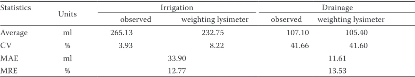
The accuracy of irrigation and drainage indirect measurements was tested (Table 1). The key points determined graphically (M2 and M3, Fig. 1) based on the records of the weighing lysimeter were con-sistent with observed data. The comparison between the irrigation amounts observed and determined by the lysimeter showed a mean absolute error (MAE)

of 33.90 ml, corresponding to a mean relative error (MRE) of 12.77%, while for the drainage the MAE was 11.61 ml representing a MRE of 13.53%.

Climate data. Air temperature and relative hu-midity were obtained from two sensors located in-side the greenhouse and recorded every minute in an automatic recording software. The daily vapour pressure deficit (VPDd) was calculated according to (Allen et al. 1998).

Leaf area. Crop variables such as leaf area (LA) and number of leaves of the bended stems (NL) of the sampling unit plants were also considered as input predictors in the daily ETc estimation model. The LA was obtained as described in (Costa et al. 2016). During the experiment, the LA of erect stems (SLA) of each sampling unit was measured once a week. A monthly count of the number of expand-ed leaves in the bent stems was made. The number of stems of the sampling units was checked two to four days a week between SLA measurements. The number of bent stems of the sampling units was also checked, between monthly measurements, and the number of expanded leaves corrected if needed.

Irrigation and drainage. The crop irrigation was managed by means of a radiation sensor. The daily Table 1. Statistics between direct (observed) and indirect irrigation and drainage measurements

Statistics

Units Irrigation Drainage

observed weighting lysimeter observed weighting lysimeter

Average ml 265.13 232.75 107.10 105.40

CV % 3.93 8.22 41.66 41.60

MAE ml 33.90 11.61

MRE % 12.77 13.53

CV – coefficient of variation; MAE – mean absolute error; MRE – mean relative error

0 0.51 1.52 2.53 3.54 4.55 5.5 195 204 217 218 231 231 232 233 234 239 241 253 255 256 289 291 292 Da ily ET c ( m m /day ) DOY

Observed Estimated LOO Lower Interval Upper Internal

0 10 20 30 40 Fre qu en cy o f e rro rs (% ) Estimated LOO y = 0.990x R² = 0.8922; n = 33 y = 0.998x R² = 0.8747; n = 33 0 1 2 3 4 5 0 0.5 1 1.5 2 2.5 3 3.5 4 4.5 5 O bs er ve d dai ly E Tc (mm /day )

Estimated daily ETc (mm/day) Estimated LOO 19.45 19.55 19.65 19.75 14: 00 14: 05 14: 10 14: 15 14: 20 14: 25 14 :30 14: 35 14: 40 14: 45 14: 50 14: 55 15: 00 Sampling unit weight (kg ) • M1 • M2 • M3 Time

Fig. 1. Example of sampling unit mass variation record: M1 – irrigation start point; M2 – irrigation end point and M3 – free drainage end point. The discontinuous line rep-resents the tendency of the mass variation to stabilize

(4)

leaching fraction of 12 substrate bags (three per sec-tor), including the four sampling units of this study, was monitored three to four times a week. The daily leaching fraction was calculated through the mean of the leaching fractions of the monitored substrate bags collected during a 24 hours period. This daily leaching fraction was used to regulate the irriga-tion in each sector. As the irrigairriga-tion system was set for automatically initiate based on a threshold of accumulated radiation, a predefined value of daily leaching fraction (40%) was considered for deter-mining the appropriate threshold. However, values of daily leaching fraction between 35 and 45% were also accepted. The collection of the leaching frac-tion was made with drainage lysimeters.

The water distribution uniformity of the green-house sectors (sectors average of 96%) in study was evaluated accordingly to NSW (2009) method. The water intake was determined indirectly by collect-ing and measurcollect-ing the volume of a “reference drip-per”, with a graduated cylinder, from one substrate bag contiguous to the monitored substrate bags.

Development of the model for daily ETc es-timation. The dependent variable ETc (range 0.4–4.6 mm/day; average (x–) = 3.0; coefficient of variation (CV) = 34.2%) was regressed against the potential predictors from climatic and crop variables. The climatic potential predictors tested were: Td – daily average air temperature (range 18.1–25.4°C; x– = 21.7; CV = 8.7%); T1 – average air temperature between midnight and 6 a.m. (range 12.7–21.9 °C; x– = 18.1; CV = 12.8%); T2 – average air temperature between 6 a.m. and the beginning of the first watering of the day (range 16.6–24.7°C; x– = 20.7; CV = 9.7%); T10 – average air temperature between the end of the drainage of the last water-ing and 9 p.m. (range 18.6–26.7°C; x– = 22.5; CV = 8.8%); T11 – average air temperature between 9 p.m. and midnight (range 14.8–22.5°C; x– = 18.8; CV = 11.6%); RHd – daily average relative humidity (range 80–100%; x– = 86.1%; CV = 5.6%); RH2 – av-erage relative humidity between 6 a.m. and the be-ginning of the first watering of the day (range 84.4– 100%; x– = 89.6%; CV = 3.8%); RH10 – average relative humidity between the end of the drainage of the last watering and 9 p.m. (range 72.5–100%; x– = 83.9%; CV = 9.1%) and VPDd (range 0.1–1.6 KPa; x– = 0.9 KPa; CV = 32.7%). Potential predictors also included the erect stem leaf area (SLA) – (range 588.3– 4345.2 cm2_{; x}– _{= 2,198.8 cm}2_{; CV = 46.7%) and the} number of leaves of the bended stems (NL) – (range

46–168; x– = 107.2; CV = 42%) on the sampling unit. Combinations such as the logarithm of SLA, LN, T2, T11 and RHd, square root of SLA, LN and square of Td, T2, T10, T11 and RHd were also tested in model development.

For the model development an initial number of 42 observations were used, from which 21% (9 ob-servations), randomly selected, were used for ex-ternal validation. Multiple stepwise regression was applied to identify robust predictors. A critical lev-el of 5% for the P-value of the Student’s t-test was set to include a variable in the model. At each vari-able inclusion step, the coefficient of determination (R2_{) value and the change in R}2_{value were also} cal-culated. Assumptions of normality, homoscedas-ticity, and the existence of multicollinearity among the independent variables were verified. The vari-ance inflation factor (VIF) and tolervari-ance (T) were calculated to assess the collinearity between the model variables. The variables with VIF > 10 and T < 0.1 were excluded from the model (Montgom-ery, Peck 1992). Inferences about the regression parameters were checked by the 95% confidence intervals and the Student’s t-tests (P < 0.05) for the null hypothesis of the regression parameters being equal to zero. The F-test (P < 0.005) was calculated to test the significance of the independent variables as a group for predicting the ETc. The regression mean prediction interval for the 95% probability level was calculated according to Montgomery, Peck (1992) and was presented graphically.

Model validation and prediction accuracy. Nine observations not used in the model parameter estimation were considered for the external valida-tion, aiming to evaluate the prediction reliability. An additional validation was applied over the full set of data (n = 33) using the “leave-one-out” (LOO) cross-validation method (Cunha et al. 2010).

The model adequacy was assessed by the percent-age of variance explained by the model, expressed by the R-square (R2_{). We used R}2

LOO to show the pro-portion of variance explained by cross validated pre-dictions. Also, several goodness-of-fit indicators were used for calibration and validation data-sets: i) resid-ual indices: the root mean square error (RMSE, mm/ day), the mean relative error (MRE, %) and the mean absolute error (MAE, mm/day), and ii) association measures based on the linear regression through the origin between pairs of observed and modeled ETc. We performed all analyses using IBM SPSS statistical software (Version 23.0., IBM Corp., USA).

(5)

RESULTS

The analysis of the coefficients of variation (CV) for the potential predictors used for modelling ranged between 3.8 % and 46.7%. The dependent variable also showed a high CV value (34%).

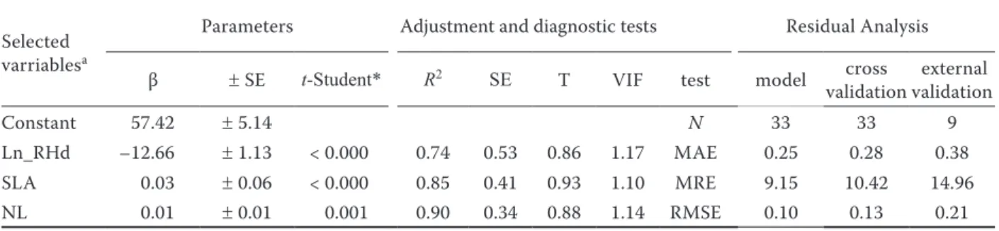
Three predictors were selected by the stepwise multiple regression model for the estimation of daily ETc: Ln_RHd, SLA and NL. Predictors and their corresponding regression coefficients for modelling the ETc are presented in Table 2. The in-tercept term and the regression coefficients of pre-dictors are significantly different from zero on the basis of t-test at 5% level (Table 2). Also, the 95% confidence interval of the regression parameters does not contain zero, which imply that they are statistically significant. The R2_{stepwise represents}

the R2_{of the regression when each model predictor} was added to the model. The model is statistically

significant on the basis of the F-test (P < 0.000). VIF was lower than 10 and T was higher than 0.1, indi-cating the inexistence of collinearity between vari-ables.

The MAE, MRE and RMSE obtained for the model validation procedures, both with external data and the cross-validation, showed good results (Table 2). For the external validation, values of 0.21 mm/day and 0.38 mm/day were obtained for RSME and MAE, respectively. Lower values were obtained in the cross-validation, with RSME of 0.13 mm/day. and MAE of 0.28 mm/day. The MRE value of the cross-validation was 10.42%, lower than the value ob-tained by the external validation (MRE = 14.96 %).

When the observed daily ETc was plotted against the modelled daily ETc (Fig. 2), the regression slope was very close to one (0.99) and the coefficient of de-termination was 89%. Moreover, the MRE between the observed and estimated daily ETc was around Table 2. Estimation of model parameter coefficients and measures of model adequacy and validation

Selected

varriablesa

Parameters Adjustment and diagnostic tests Residual Analysis

β ± SE t-Student* R2 _SE _T _VIF _test _model cross

validationvalidation external

Constant 57.42 ± 5.14 N 33 33 9

Ln_RHd –12.66 ± 1.13 < 0.000 0.74 0.53 0.86 1.17 MAE 0.25 0.28 0.38

SLA 0.03 ± 0.06 < 0.000 0.85 0.41 0.93 1.10 MRE 9.15 10.42 14.96

NL 0.01 ± 0.01 0.001 0.90 0.34 0.88 1.14 RMSE 0.10 0.13 0.21

a_{selected variables using the stepwise regression method (P < 0.05) and the value of tolerance value (T) and variance}

infla-tion factor (VIF) were logarithm of daily average relative humidity (Ln_RHd), erect stem leaf area (SLA), and number of leaves of the bended stems (NL), the other variables included in the model were not considered statistically significant by the stepwise regression method; *probability associated with the Student’s t-test

0 10 20 30 40 < 5% 5–10 10–15 –20% > 20% Fre qu en cy o f e rro rs (% ) Classes of error (%) Estimated LOO y = 0.990x R² = 0.8922; n = 33 y = 0.998x R² = 0.8747; n = 33 0 1 2 3 4 5 0 0.5 1 1.5 2 2.5 3 3.5 4 4.5 5 O bs er ve d dai ly E Tc (mm /day )

Estimated daily ETc (mm/day)

Estimated LOO 19.45 19.55 19.65 19.75 14: 00 14: 05 14: 10 14: 15 14: 20 14: 25 14 :30 14: 35 14: 40 14: 45 14: 50 14: 55 15: 00 Sampling unit weight (kg )

•

M1

•

M2

•

M3 Time

Fig. 2. Regression through the origin between observed and modelled (estimated and LOO – “leave-one-out” cross-validation method)) daily crop evapotranspiration. The regression 1 : 1 is represented by the dashed line

(6)

9.1%, corresponding to a MAE of 0.25 mm/day and RMSE of 0.10 mm/day. Similar results were ob-tained when comparing the cross validation ETc values with the observed daily ETc values (regres-sion slope close to one and coefficient of determi-nation of 87%).

Daily observed and modelled ETc values (both es-timated and using the LOO cross validation) were compared, showing a good similarity between the sets of data (Fig. 3).The model was able to accom-modate a wide range of ETc values (CV = 34.2%), which included the minimum value of 0.4 mm/day and a maximum of 4.61 mm/day. The data set for the model development covered the full crop cycle, thus contributing to the model robustness.

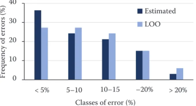
Additionally, in 79% (LOO cross validation) and 82% (estimation) of the cases, the errors between observed and modelled values were lower than 15%

(Fig. 4), all consistently inside the prediction inter-val (Fig. 3).

DISCUSSION

When analysing the CV of the potential predic-tors used for the daily ETc modelling, we concluded that, with the exception of the variables Td, T2, T10, RHd, RH2 and RH10, there was a marked variabil-ity in the selected descriptors, which allowed the formulation of ETc estimates over a wide validation interval and contributed to the model robustness.

In the daily ETc model (Table 2), the regression coefficients for crop predictors related with the LA are positive while for the climatic predictors is negative, thus consistent with what would be ex-pected for their impact on ETc (Allen et al. 1998). Hence, an increase in the LA and a decrease in the RHd results in an increase in the ETc. The model presented a satisfactory fit when using solely the RHd, with R2 _{values of 0.74, which increased to} 0.90 when the variables related with crop predic-tors were added to the model. Thus, 90% of the dai-ly variability of ETc in different crop stages can be explained by the three predictors. The selection of these predictors highlights the importance of crop variables such as LA (Stanghellini 1987; Baille et al. 1994; Suay et al. 2003). Cut roses, unlike most crops, are continuously harvested, and thereby ex-hibit a large time-variability of their transpiration area, making LA an important parameter when modelling roses ET (Raviv, Blom 2001). The RHd 0 0.51 1.52 2.53 3.54 4.55 5.5 195 204 217 218 231 231 232 233 234 239 241 253 255 256 289 291 292 Da ily ET c ( m m /day ) DOY

Estimated LOO 19.45 19.55 19.65 14: 00 14: 05 14: 10 14: 15 14: 20 14: 25 14 :30 14: 35 14: 40 14: 45 14: 50 14: 55 15: 00 Sampling unit weight • M1 • M3 Time

Fig. 3. Overall comparison between observed and modelled (estimated and predicted – LOO) daily ETc for 33 obser-vations. The predicted was obtained from the leave-one-out cross validation procedure (LOO). External thicker lines are the prediction interval (α = 95%)

DOY – day of the year

Estimated LOO 19.45 19.55 19.65 19.75 14: 00 14: 05 14: 10 14: 15 14: 20 14: 25 14 :30 14: 35 14: 40 14: 45 14: 50 14: 55 15: 00 Sampling unit weight (kg ) • M1 • M2 • M3 Time

Fig. 4. Frequency levels of errors between each pair of observed and modelled (estimated or predicted) daily crop evapotranspiration

112

Original Paper Horticultural Science (Prague), 46, 2019 (2): 107–114

(7)

is also a key parameter for the ET demand (Mpusia 2006)(Mpusia 2006). Although the VPD (inversely proportional to air humidity) is considered one of the main factors affecting greenhouse crop tran-spiration, along with solar radiation and stomatal resistances (Raviv, Blom 2001; Katsoulas, Kit-tas 2011), it was not selected as a predictor for our model. Similarly, the VPD did not improve regres-sion models for estimating crop transpiration in a glasshouse study with roses (Baas, Van Rijssel 2006). The model developed in our study presented a R2_{very similar to the values obtained by (Suay et} al. 2003) and (Baas, Van Rijssel 2006) although a lower number of observations were used in our study when compared to (Suay et al. 2003).

When the observed daily ETc values were plotted against the modelled daily ETc, the regression slope was close to one (0.99) and the coefficient of determination was 89%, showing the model’s ability to estimate daily ETc with high accuracy and precision (Fig. 2).

The model good predictive performance is also supported by the results obtained when compar-ing the LOO cross validation ETc values with the observed daily ETc values (Fig. 2; regression slope close to one and the coefficient of determination of 87%). The similarity between observed and mod-elled ETc data (Fig. 3) also indicates good perfor-mance of the developed model.

When compared to other simplified models used to determine the transpiration of roses (Suay et al. 2003; Baas, Van Rijssel 2006; Mpusia 2006) the developed model presents the advantage of using less predictors, which can be more easily obtained, without a large cost-investment. In the simpli-fied roses transpiration models used by Suay et

al. (2003), Mpusia (2006) and Baas and Van

Ri-jssel (2006), radiation and VPD inputs or energy input from heating system are used. However, in an operational context, most greenhouses in the Mediterranean area have minimal climate control equipment (Montero et al. 2011), making data collection of such variables a difficult task. Our model presents the advantage of using more user-friendly inputs, such as dRH, a common variable controlled by producers. The main advantage and novelty of our model is its applicability to different stages of the crop development, by using the crop parameter SLA. The non-destructive method for determining the SLA for the cultivar ‘Red Naomi’ developed by Costa et al. (2016) allows the model to accommodate the variation of the LA throughout

the entire crop cycle instead of being limited to a specific stage of crop development. This advantage is particularly relevant in roses, where harvesting is continuous. However, the determination of crop predictors (SLA and NL) selected by the model is time consuming, which can cause some constrains.

The developed model, like the ones above men-tioned, has the disadvantage of using predictors that can only be determinate at the end of the day (in our study, is RHd). However, relative humidity inside the greenhouse can be predicted, primarily from external relative humidity, ventilation rate and ET (Litago et al. 2005). In either case, the RHd can be adjusted throughout the day, based on data from the greenhouse sensor. Future studies should be undertaken to test the robustness of the model in different greenhouse conditions, other cut rose cultivars, and types of greenhouses.

Acknowledgements

The authors thank Sara Gonçalves for her help. We also thank Floralves Company and Sérgio Alves.

References

Allen R.G., Pereira L.S., Howell T.A., Jensen M.E. (2011): Evapotranspiration information reporting: I. Factors governing measurement accuracy. Agricultural Water

Management, 98: 899–920.

Allen R.G., Pereira L.S., Raes D., Smith M. (1998): Crop evapotranspiration: guidelines for computing crop water requirements. FAO: Irrigation and Drainage Paper No. 56., Food and Agriculture Organization of the United Nations. Baas R., van Rijssel E. (2006): Transpiration of glasshouse

rose crops: Evaluation of regression models. Proc III In-ternational Symposium on Models for Plant Growth, En-vironmental Control and Farm Management in Protected Cultivation, Leuven, Belgium: 547–554.

Bacci L. et al. (2011): Modelling evapotranspiration of container crops for irrigation scheduling. In: Evapo-transpiration – From Measurements to Agricultural and Environmental Applications. Croatia, InTech: 263–282. Baille M., Baille A. and Delmon D. (1994): Microclimate and

transpiration of greenhouse rose crops. Agricultural and

Forest Meteorology, 71: 83–97.

Bayer A., Mahbub I., Chappell M., Ruter J., van Iersel M.W. (2013): Water use and growth of Hibiscus acetosella ‘Panama Red’ grown with a soil moisture sensor-controlled irrigation system. Hortscience, 48: 980–987.

(8)

Costa A., Pôças I., Cunha M. (2016): Estimating the leaf area of cut roses in different growth stages using image process-ing and allometrics. Horticulturae, 2: 6.

Cunha M., Marcal A., Silva L. (2010): Very early prediction of wine yield based on satellite data from vegetation.

International Journal of Remote Sensing, 31: 3125–3142.

Farahani H.J., Howell T.A., Shuttleworth W.J., Bausch W.C. (2007): Evapotranspiration: progress in measurement and modeling in agriculture. Transactions of the ASABE, 50: 1627–1638.

Gavilan P., Ruiz N., Lozano D. (2015): Daily forecasting of reference and strawberry crop evapotranspiration in green-houses in a Mediterranean climate based on solar radiation estimates. Agricultural Water Management, 159: 307–317. Harel D., Sofer M., Broner M., Zohar D., Gantz S. (2014):

Growth-stage-specific Kc of greenhouse tomato plants grown in semi-arid Mediterranean region. Plants Grown

in Semi-Arid Mediterranean Region, 6: 132–142.

Katsoulas N., Kittas C. (2011): Greenhouse crop transpiration modelling. In: Evapotranspiration – from Measurements to Agricultural and Environmental Applications. Croatia, InTech: 311–328.

Litago J. et al. (2005): Statistical modelling of the microclimate in a naturally ventilated greenhouse. Biosystems Engineer-ing, 92: 365–381.

Montero J.I., van Henten E.J., Son J.E., Castilla N. (2011): Greenhouse Engineering: New Technologies And Ap-proaches. Acta Horticulturae (ISHS), 893: 51–63. Montgomery D., Peck A. (1992): Introduction to linear

re-gression analysis. New York, John Wiley and Sons USA. Morille B., Migeon C., Bournet P.E. (2013): Is the Penman–

Monteith model adapted to predict crop transpiration

un-der greenhouse conditions? Application to a New Guinea Impatiens crop. Scientia Horticulturae, 152: 80–91. Mpusia P. (2006): Comparison of water consumption between

greenhouse and outdoor cultivation. [Master Thesis.] International Institute for Geo-information Science and Earth Observation in Netherlands: 1–75.

NSW (2009): Preventing pests and diseases in the greenhouse – Distribution uniformity of irrigation (Fact sheet).

Avail-able at http://www.dpi.nsw.gov.au/

Orgaz F., Fernández M.D., Bonachela S., Gallardo M., Fereres E. (2005): Evapotranspiration of horticultural crops in an unheated plastic greenhouse. Agricultural Water

Manage-ment, 72: 81–96.

Raviv M., Blom T.J. (2001): The effect of water availability and quality on photosynthesis and productivity of soilless-grown cut roses. Scientia Horticulturae, 88: 257–276. Stanghellini C. (1987): Transpiration of greenhouse crops:

an aid to climate management. [Ph.D. Thesis.] Instituut voor Mechanisatie in Wageningen: 1–161.

Suay R. et al. (2003): Measurement and estimation of transpi-ration of a soilless rose crop and application to irrigation management. Proc VI Int Symp on Protected Cultivation in Mild Winter Climate: Product and Process Innovation.

Acta Horticulturae (ISHS), 614: 625–630.

Villarreal-Guerrero F., Kacira M., Fitz Rodríguez E., Kubota C., Giacomellin G.A., Linker R., Arbel A. (2012): Compari-son of three evapotranspiration models for a greenhouse cooling strategy with natural ventilation and variable high pressure fogging. Scientia Horticulturae, 134: 210–221.

Received for publication August 22, 2017 Accepted after corrections July 27, 2018