The impact of credit rating agencies downgrades on european stock markets during the financial crisis of 2008

THE IMPACT OF CREDIT RATING AGENCIES

DOWNGRADES ON EUROPEAN STOCK MARKETS

DURING THE FINANCIAL CRISIS OF 2008

Inês Nunes Pedras

Dissertation submitted as partial requirement for the conferral of Master in Finance

Supervisor:

Prof. Paulo Viegas de Carvalho, Assistant Professor, ISCTE Business School, Departament of Finance

I

R

Uma das crises financeiras mais graves até agora começou nos Estados Unidos, atingindo o pico após o colapso do banco de investimento Lehman Brothers, no outono de 2008. As consequências foram catastróficas, atingindo todo o mundo. É o caso da crise da dívida soberana da Zona Euro.

As agências de notação de crédito foram fortemente criticadas durante ambas as crises. Acredita-se que as suas notações possam ter provocado a primeira e que os seus

downgrades podem ter piorado a situação da segunda.

Este trabalho pretende analisar o papel das agências de notação de crédito em crises recentes, avaliando em particular se as notações de crédito soberano tiveram um impacto sobre os mercados de ações. Um estudo de evento é realizado a fim de estudar a reação dos mercados de ações antes e após os anúncios das três principais (S&P, Moody’s e Fitch).

Os resultados indicam que apenas os downgrades têm retornos anormais significativos, e que estes são negativos. Além disso, há evidências de que os mercados não antecipam, mas reagem aos anúncios. Das três agências examinadas, apenas os downgrades da S&P e Fitch resultam em descidas significativas no mercado. Apenas os downgrades durante os primeiros cinco anos dos dez em análise tiveram um impacto negativo significativo. Apesar destes anos abrangerem tanto a crise financeira global como o início da crise na zona do euro, a maioria dos downgrades ocorreram nos últimos cinco. Finalmente, os mercados de ações da Bélgica e da Itália foram os únicos afetados pelos downgrades noutros países.

Palavras-chave: Agências de Notação de Crédito, Risco Soberano, Estudo de Eventos,

Crises Financeiras

II

A

One of the most severe financial crises until now started in the United States, reaching the peak after the collapse of the investment bank Lehman Brothers, in the fall 2008. The consequences were catastrophic, extending to all over the world. An example is the case of the Eurozone sovereign debt crisis.

Credit Rating Agencies were heavily criticized during both crises, the global financial crisis, and the Eurozone sovereign debt crisis. Many people believe that their grades have triggered the first crisis, and that their downgrades may have worsened the situation in the latter crisis.

This paper aims to analyse the role of credit rating agencies in the recent crisis, particularly whether sovereign credit ratings had an impact on the stock markets. An event study is performed on order to investigate the reaction of stock markets before and after announcements from the three main rating agencies (S&P, Moody’s and Fitch).

Results indicate that only downgrades have significant abnormal returns, and that they are negative. Furthermore, there is evidence that markets do not anticipate, but react instead to the announcements. Of the three credit rating agencies examined, only S&P and Fitch rating downgrades result in significant market falls. Only downgrades during the first five years of the ten under analysis reveal a significant negative impact. Despite these years encompass both the global financial crisis as the beginning of the crisis in the Eurozone, most of the downgrades occurred in the last five years. Finally, Belgian and Italian stock markets were the only affected by downgrades in other countries.

Keywords: Credit Rating Agencies, Sovereign Risk, Event Study, Financial Crises JEL Classification: G14, G24

III

A

I would like to start by thank Professor Paulo Viegas de Carvalho for accepting to be my supervisor and coordinate me throughout this journey. I truly appreciate all the availability for discussion as well all the support shown during the development of this paper.

I would also like to thank my long-time friend Tetyana for her friendship and all the availability and assistance provided, especially, in the last few months.

A special thanks to Martin for all the patience and time spent encouraging and supporting me, as well as for his important comments and useful advices.

Finally, I would like to thank to my family. To my father, that was always there for me and encouraged me not only to study but also to be happy and follow my dreams. To my sisters, that make me want to always be better and be a good role model to them. And to my grandparents Zezé and Quim, to whom I dedicate this dissertation, for all the unconditional support and love.

IV

T

C

2.1. Credit Rating Agencies ... 3

2.1.1. Definition and Role ... 3

2.1.2. From “Investor Pays” to “Issuer Pays” Model ... 4

2.1.3. Process ... 5

2.1.4. Scale ... 5

2.2. Sovereign Ratings ... 7

2.2.1. Determinants ... 7

2.3. Financial Crisis of 2008 ... 10

2.3.1. Iceland Financial Crisis ... 12

2.3.2. Eurozone Debt Crisis ... 12

2.4. Overview of related research ... 15

3. Data ... 18

3.1. Rating Announcements ... 18

3.2. Stock Market Returns ... 20

4. Methodology ... 22

4.1. Event Study ... 22

4.1.1. Cumulative Abnormal Returns ... 25

4.1.2. Average Abnormal Returns ... 25

4.1.3. Cumulative Average Abnormal Returns ... 26

5. Empirical Results ... 28 5.1. Downgrades vs Upgrades ... 28 5.2. Downgrades by Agency ... 32 5.3. Downgrades by Period ... 34 5.4. Contagion of Downgrades ... 38 6. Conclusion ... 42 References ... 44 Appendix ... 48

V

T

F

Table 2.1. Credit Rating Scale ... 6

Table 2.2. Sample Statistics by Broad Letter Rating Categories ... 10

Table 3.1. Number of Rating Announcements by Type and by Agency ... 18

Table 3.2. Index Value Appreciation (in %) ... 20

Table 5.1. Average Abnormal Returns and respective t-test value by type of announcement ... 29

Table 5.2. Cumulative Average Abnormal Returns and respective t-test value by type of announcement ... 30

Table 5.3. Average Abnormal Returns and respective t-test value by agency ... 32

Table 5.4. Cumulative Average Abnormal Returns and respective t-test value by agency ... 33

Table 5.5. Average Abnormal Returns and respective t-test value by period ... 35

Table 5.6. Cumulative Average Abnormal Returns and respective t-test value by period ... 36

Table 5.7. Average Abnormal Returns and respective t-test value by country ... 39

Table 5.8. Cumulative Average Abnormal Returns and respective t-test value by country ... 40

Figure 2.1. Long-term Interest Rates ... 13

Figure 3.1. Number and Type of Sovereign Rating Changes per Year ... 19

Figure 5.1. Cumulative Average Abnormal Returns by Type of Announcement ... 31

Figure 5.2. Cumulative Average Abnormal Returns by Agency... 34

1

1. I

The global financial crisis is considered by several authors to have been the most severe financial crisis since the Great Depression (see, for instance, Eigner and Umlauft, 2015). It reached the peak after the collapse of the investment bank Lehman Brothers, in September 2008, but its origin is usually associated to a problem in the particular segment of the U.S. mortgage market – the subprime mortgage market – years earlier. The adverse effects of the subprime crisis were felt not only in the United States, but in the whole world. The Eurozone debt crisis is one of those effects.

Following the global financial crisis, the financial markets started pressing certain Eurozone countries, like Greece, Ireland and Portugal, due to their budgetary problems and high levels of sovereign debt. As soon as it became less clear whether these countries would have the capacity to meet their credit commitments, the rating agencies started to downgrade their sovereign ratings. As a consequence, the three main credit rating agencies (S&P, Moody’s and Fitch) were heavily criticized, and some politicians and press also suggested that the agencies decisions intensified and could even have extended the crisis.

The previous literature that studied the impacts of credit rating announcements is extensive, in most cases concluding that credit rating agencies (CRAs) opinions and decisions influence the financial markets (e.g., Kaminsky and Schmulker, 2002; Kräussl, 2003). However, studies about the impact of the announcements of the rating agencies on stock markets in the recent crises are scarce.

The purpose of this paper is to assess the impact of CRAs announcements, especially the downgrades, on certain European stock markets during the crises periods, i.e. from 2006 to 2015. In order to get a conclusion, we use the event study methodology, a common approach when the impact of a certain event needs to be assessed. This study first analyses the differences of the abnormal returns after an upgrade and after a downgrade. Then, the impact of downgrades is analysed in more detail, first, by examining the differences between the three main agencies, and, second, by period of time. As a final point, the cross-country contagion of downgrades is also studied.

The main findings are the following. Credit rating agencies downgrades have a significant negative impact on the stock markets and, among the three main agencies, only Moody’s

2 downgrades have no significant impact. Although most of the downgrades have occurred during the Eurozone crisis, they only had a significant impact in the period that encompasses the global financial crisis, that is, between 2006 and 2010. From the twelve countries analysed, only two had their stock markets affected by downgrades in other countries: Belgium and Italy. As they are both from Eurozone, we conclude that contagion is limited to neighbouring countries.

This paper consists of six sections besides the introduction. Section 2 focuses on the background of the credit rating agencies industry, the sovereign ratings and the global financial crisis. This section also reviews previous literature related to the impact of the credit agencies. In Section 3, we present a brief analysis of the dataset and, in Section 4, we detail the methodology. Section 5 analyses the empirical results. Section 6 presents the main limitations of the study, and Section 7 concludes.

3

2. L

R

2.1. CREDIT RATING AGENCIES 2.1.1. Definition and Role

A Credit Rating Agency is a private company that evaluates debtors (governments, financial, and non-financial firms) and the financial instruments they issue. In other words, CRAs rate the capability and disposition of a debtor to pay a debt, i.e., they evaluate its creditworthiness.

In 1909, John Moody published the first rating book, focusing on U.S. railroad bonds. Soon after, Poor’s Publishing Company, in 1916, the Standard Statistics Company, in 1922, and the Fitch Publishing Company, in 1924, followed the initiative of Moody’s firm (White, 2010).

Nowadays, there are three firms that jointly dominate 95 percent of the worldwide credit rating industry: Standard & Poor’s Rating Services (S&P) and Moody’s Investors Service hold 40 percent each, while Fitch Ratings has 15 percent of the market. These three big and global acting firms are wide in their product coverage, but most CRAs are regional or product-type specialists (Haan and Amtenbrink, 2011). There are around 150 other CRAs specialized in rating various instruments, industries and/or national markets (White, 2010), and the number is expected to increase in the future, especially in the less developed markets.

According to Basel Committee on Banking Supervision (2000: 14), “there is a wide disparity in size among rating agencies, as measured by the number of employees or number of ratings assigned”. However, the latter measure can be considered ambiguous, since the number of ratings assigned is dependent on how they are determined. For instance, an agency using an intensive analytical work (i.e. based on the judgement by credit analysts) on the institution being evaluated will spend more time and resources than another that uses publicly available data as input to a statistical model.

Despite these differences, CRAs play an important role in financial markets. For instance, they mitigate problems of asymmetric information between market participants (issuers, investors, and regulators) (Norden and Weber, 2004). This credit risk information is produced and distributed, and can then be used in the decision-making process. For

4 example, State governments seek ratings with the intention of attracting foreign investors, and so finance public debt.

Nevertheless, their decisions can also prove to be harmful. Because of their strong influence on interest rates – a downgrade may lead to higher interest rates (see, for instance, El-Shagi and Schweinitz, 2016) –, they could increase the volatility and compromise the financial stability of the markets.

2.1.2. From “Investor Pays” to “Issuer Pays” Model

After John Moody published in 1909 the first book of ratings, the credit ratings’ industry became dominated by the "investor pays" model. The agencies provided public ratings of an issuer free of charge; however the ratings were subscription-based and were only available to investors who had paid for them.

In the early 1970s, the remuneration model of the main rating agencies changed from an “investor pays” to an “issuer pays” model (Cantor and Packer, 1994). In the “issuer pays” model, the entities issuing bonds pay the credit rating agency for their ratings. Nowadays, this compensation model is the dominant one in the credit rating industry, representing more than two-thirds of total agencies revenues (Haan and Amtenbrink, 2011).

Regardless of the transition motives, White (2010: 215) states that the change on the model adopted “opened the door to potential conflicts of interest: a rating agency might shade its rating upward so as to keep the issuer happy and forestall the issuer’s taking its rating business to a different rating agency”.

This reasoning may, however, be challenged. On the one hand, there are numerous potential bond issuers (corporates and governments) in the market. This makes the damage by any single issuer to change to a different rating agency not so significant. On the other hand, information on bond issuers whose “plain vanilla1_{” debt was being rated}

is quite transparent. Therefore, any error in rating assessment would be quickly detected,

1 _{Plain vanilla indicates the standard version of a financial instrument, namely bonds, options, futures, and}

5 thus damaging the rating agency’s reputation – a critical factor for their business sustainability.

2.1.3. Process

Each CRA has its own unique rating procedures, but the general process is quite similar across most of them. According to Moody’s Investors Service (2016), before starting the rating process, there is an introductory meeting with the aim of introducing the agency and provide important information about the whole process and products. Only when the issuer is ready to move forward and sign its application, the process can start.

First of all, relevant information on the issuer or obligation is collected by the assigned analyst(s). It may include both financial and non-financial data and can be retrieved from publicly available sources or provided by the Issuer. The information obtained is then analysed using relevant credit rating methodologies and taking into account quantitative and qualitative factors.

After a management meeting with the issuer, where its strengths and weaknesses as well as the industry trends are discussed, the lead analyst formulates a recommendation for consideration by a rating committee. Once the rating committee reaches a decision, the lead analyst contacts the issuer to inform about the rating decision.

Finally, the credit rating is released. Typically, the announcements are published on the respective Credit Rating Agency’s website, and distributed to the major financial newswires via press release.

Credit ratings can be modified if the analyst’s opinion about the creditworthiness of the issuer or issue changes, since he continues monitoring the credit rating.

2.1.4. Scale

When the Securities and Exchange Commission was created, in 1934, corporations had to standardize their financial statements. Consequently, these statements started to appear in the form of “ratings”.

Nowadays, S&P and Fitch, and Moody’s use the two main scales, where credit ratings are classified on a scale of letters (table 2.1). Modifiers are then attached to distinguish

6 ratings within classification. S&P and Fitch use pluses and minuses, while Moody’s uses numbers. Both scales can be divided in two parts: “investment grade”, going from a minimal risk (AAA/Aaa) to a moderate credit risk (BBB-/Baa3), and “speculative grade” (from BB+/Ba1 to below), denoting a risky investment. Summing up, the less risk a CRA perceives in an Issuer or a bond, the better will be the respective rating.

Table 2.1. Credit Rating Scale

Source: IMF

Usually, an agency signals in advance its intention to ponder rating changes, using “outlooks” and “watchlists”. While watchlists concentrates on shorter term – three months, on average –, an outlook represents the opinion of an agency on a creditworthiness change over the medium time horizon (Haan and Amtenbrink, 2011).

7 2.2. SOVEREIGN RATINGS

Like other credit ratings, sovereign ratings are assessments of the creditworthiness of a borrower; in this case, the borrower is a sovereign entity.

According to Cantor and Packer (1996: 38), “sovereign ratings are important not only because some of the largest issuers in the international capital markets are national governments, but also because these assessments affect the ratings assigned to borrowers of the same nationality”.

2.2.1. Determinants

The three main credit rating agencies make use of several economic, social, and political factors to sustain their sovereign credit ratings. However, it is difficult to identify the relationship between their criteria and actual ratings (Bissoondoyal-Bheenick, 2005). On the one hand, some factors are not quantifiable. On the other hand, even for quantifiable factors, it is difficult to determine the relative weights assigned by each agency, since these depend on a large number of criteria.

Cantor and Packer (1996) use regression analysis to measure the relative significance of a set of variables mentioned in rating agencies’ reports as determinants of sovereign ratings. We choose six of them to demonstrate the differences between each sovereign rating level: per capita income, GDP growth, inflation, sovereign debt, fiscal balance, and external balance.

Per capita income

Per capita income measures the average income earned per person in a certain country. It is often used to evaluate the standard of living and quality of life within a country. The higher the potential tax basis of a country, the greater will be the ability of its government to repay debt.

GDP growth

The economic growth rate provides a perception of the general direction and magnitude of development of an economy’s capacity in producing goods and services. The greater

8 is the rate of economic growth, the better will be the possibility of the existing debt to be paid more easily over time.

Inflation

Inflation is a sustained increase in the general price level of goods and services. As a result, with high inflation the purchasing power of a unit of the national currency falls and, consequently, it may lead to social problems and political instability.

The opposite of inflation, deflation, can be just as bad (or even worse) for the economy than high inflation. It can be caused by a decrease in government, personal or investment spending, and it can lead to an increase of unemployment due to a lower level of demand in the economy, which may lead to an economic depression.

Central banks attempt to limit inflation, and avoid deflation, with the intention of keeping the economy running efficiently. For that purpose, the European Central Bank aims to maintain inflation rates below, but close to, 2%.

Sovereign debt

Sovereign debt is the accumulation of annual budget deficits. On the one hand, this is a way for countries to get funds to improve their standard of living and boost economic growth. On the other hand, this is also an alternative to diversify investments by buying a country’s government bonds.

However, when debt rises up to or above a level deemed as critical, investors usually start requiring higher interest rates to compensate the greater risk. With the rise in interests, it becomes more expensive for a country to refinance its existing debt, which, in extreme circumstances, may pressure a situation of credit default. As an example, in 2001, Argentina declared default due to its £94 billion external debt (Arie and Cave, 2001). Governments must be careful in finding the breaking point of their debt: it should be large enough to stimulate economic growth, but only as long as interest rates are kept low.

Fiscal balance

The budget balance is the overall difference between government income and expenditures. A positive balance, i.e. when income exceeds expenditures, means a budget

9 surplus, denoting that the government is being efficient and as such it can pay off debt, save, or invest. On the contrary, a negative balance, i.e. a budget deficit, requires financing by borrowing money, which may complicate the payment of the existing debt and even may increase its value. Normally, the deficit, as a percentage of GDP, is expected to decrease in times of economic prosperity due to higher economic activity stimulating collection of taxes. In this sense, governments can counter budget deficits by promoting economic growth, thus potentially increasing tax collection, provided that spending remains under control.

External balance

The current account balance is defined as the sum of the trade balance (net exports of goods and services), net primary income, and net secondary income. A country’s current account balance is influenced by several factors, namely its trade policies, inflation rate, exchange rate, etc.

The trade balance is usually the major determinant of the current account surplus or deficit. If there is a surplus, it indicates that the country is a net lender from abroad. On the contrary, if there is a deficit, it means that the country is a net borrower from the rest of the world.

Table 2.2 below shows the relationship between the previous variables and the different sovereign rating levels in 2013. The countries included in this analysis are the twelve countries whose stock markets will be later analysed. Currently, Austria, Germany and Netherlands share the highest average rating level – AAA. Belgium and France have a rating AA, whereas Iceland, Ireland, Italy and Spain share a BBB. Portugal and Greece are the two countries with the lowest average rating levels – BB and -B, respectively. Numerical values were assigned as follows: AAA/Aaa = 22, AA+/Aa1 = 21, and so on through D = 1. The country’s average rating is then calculated, using the three numerical values denoting ratings by S&P, Moody’s and Fitch for that country on the last day of 2013.

10

Table 2.2. Sample Statistics by Broad Letter Rating Categories

Variable Rating

AAA AA A BBB BB B < B Per capita income (thousands of $) 48,9 41,75 - 37,7 27,55 - 27,05

GDP growth (annual %) 1,53 1,21 - 0,04 -1,25 - -6,28

Inflation (annual %) 2,08 2,01 - 2,48 2,05 - 2,15

Sovereign debt (% of GDP) 72,94 90,71 - 104,40 118,63 - 147,73

Fiscal balance (% of GDP) -2,19 -3,70 - -7,03 -7,45 - -10,65

External balance (% of GDP) 4,46 -0,43 - -0,43 -4,20 - -6,15

Source: World Bank

As can be seen, the data indicates a clear relationship between the different variables and the 5 rating levels presented. The best rated countries have, in fact, a higher income per capita, a higher growth rate of GDP, a public debt below the value of GDP, a public deficit reduced and an external balance close or above zero.

In contrast, the speculative grade countries have a clear contraction of their economies: a negative GDP growth, a public debt well above the value of GDP, a public deficit higher than 7% and a deficit in the external balance above 4%. All these factors will possibly contribute to worsen a country’s debt and hinder its payment. This tends to affect the sovereign credit rating, since it is an assessment of the risk associated with investing in a particular country.

The only variable that seems not to have a relationship with the rating level is inflation. All levels reveal an inflation close to the level desired by the European Union (2%), except the BBB level that shows an inflation slightly higher.

2.3. FINANCIAL CRISIS OF 2008

A financial crisis is characteristically a multidimensional event which is difficult to describe by a single indicator (Claessens and Kose, 2013).

The financial crisis of 2008 was not an overnight situation. However, as stated by the Financial Crisis Inquiry Commission (2011: xvi), “it was the collapse of the housing bubble — fuelled by low interest rates, easy and available credit, scant regulation, and

11 toxic mortgages — that was the spark that ignited a string of events, which led to a full-blown crisis in the fall of 2008”.

The crisis reached the height after the collapse of the investment bank Lehman Brothers and the imminent breakdown of the insurance American International Group (AIG) in September 2008. The lack of transparency of the balance sheets of major financial institutions, along with a tangle of interconnections between institutions perceived as “too big to fail2”, spread the panic on the financial markets.

It is believed that the rating agencies may have played a crucial role in this crisis. For the Financial Crisis Inquiry Commission (2011, xxv), the three major rating agencies were “key enablers” and this financial crisis could not have occurred without them, since that “mortgage-related securities at the heart of the crisis could not have been marketed and sold without their seal of approval”.

Take the example of Moody’s on the US market. From 2000 to 2007, Moody's rated nearly 45,000 mortgage-related securities as the highest rating level – Aaa. In 2006, 30 mortgage-related securities were rated with this level every working day. From these, 83% were eventually downgraded.

Since these securities had been approved and were well rated by the rating agencies, investors naively relied on them, leading to “a massive mispricing of risk, whose correction later detonated the crisis” (Pagano and Volpin, 2010:1).

Credit rating agencies were also criticised for downgrading European sovereigns and intensifying financial problems of Eurozone countries like Portugal or Greece. On 6 July 2011, the European Commission spokesman, Amadeu Altafaj, stated about the Portuguese ratings downgraded back then: “the timing of Moody's decision is not only questionable, but also based on absolutely hypothetical scenarios which are not in line at all with implementation. This is an unfortunate episode and it raises once more the issue of the appropriateness of behavior of credit rating agencies” (Reuters, 2011). The until

2 _{“Too big to fail” is the idea that a certain business has become so outsized and, consequently, vital to the}

economy that a government will do whatever it necessary to prevent its bankruptcy, as failure will have a disastrous impact on the country’s economy.

12 then Commission President, Manuel Barroso, further stated that Moody's downgrade “added another speculative element to the situation” (BBC, 2011).

2.3.1. Iceland Financial Crisis

During the global financial crisis, the three largest Icelandic banks – Kaupthing Bank, Landsbanki, and Glitner Bank – collapsed and, consequently, were nationalized. After that, the value of its currency – the Iceland krona – fell down (see appendix 2), the stock market decreased approximately 95 percent (see appendix 3). Moreover, rating agencies cut sovereign credit rating until junk status, foreign investors started leaving the country and almost every business on the country went bankrupt (Anderson, 2015).

After a request to the IMF of a $2.1 billion arrangement has been accepted, in November 2008 (IMF, 2008), Iceland began its surprising recovery period. The quick restoration of the banking system and early steps to accelerate sovereign debt restructuring, as well the good use of its natural resources, were important factors of its remarkable recovery after the devastating 2008 crisis (Hammar, 2015).

The fact that the country has its own currency also helped, because devaluation was made possible autonomously, which allowed more competitive exports and more expensive imports.

According to World Bank’s data, in 2011, the Iceland inflation and deficit continued to reduce and the GDP finally started to grow. Once its financial capacity showed signs of improvement, the country chose to anticipate the payment of the debt to the IMF. The last payment was held in October 2015 (IMF, 2015).

2.3.2. Eurozone Debt Crisis

Sovereign debt is a central government's debt. It is an accumulation of a government's annual deficits and it shows how much more a government spends than it obtains in revenue over time. A sovereign debtcrisis occurs when the situation becomes uncontrollable and the country is unable to pay its obligations. This occurred to some Eurozone countries, such as Greece, Ireland, Portugal, and Spain, following the Global Financial Crisis.

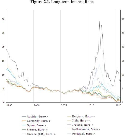
13 After the creation of the Euro as one common currency in 1999, it was assumed that big economies, like Germany and France, would never allow a member state to go “bankrupt” – “too big to fail” again – because that would have serious implications on the complete Eurozone financial system. As a result, and since interest rates are related to the risk, countries like Greece and Portugal were able to borrow money at much lower rates (see figure 2.1) and ended up overspending and increasing sovereign debt (see appendix 4). When the subprime crisis hit first the US, especially when one of the largest investment banks, supposedly “too big to fail”, collapsed, investors and credit rating agencies became sceptical about the risk of some European countries. If Lehman Brothers went bankrupt, the possibility that some countries may also face credit default (even if they were in the EU) gained relevance.

Figure 2.1. Long-term Interest Rates

14 The consequence was that ratings of countries like Greece, Ireland and Portugal were downgraded, their government bond yields jumped (see figure 2.1) and, suddenly, refinancing the debt became expensive and unsustainable. As a result, these countries ended up asking for financial assistance (see Central Bank of Ireland, 2016 and Banco de Portugal, 2016).

Greece Debt Crisis

The Greek debt crisis was the most severe of the Eurozone countries. It started when the country’s budget deficit (in % of GDP) for 2009 was revised from 3.7% to 12.5%, well above the 3% ceiling for the Eurozone countries (European Comission, Stability and growth pact, 2016c). Later, Eurostat showed that the deficit was in fact 15.4%, more than five times the ceiling.

Reflected in the huge increase in interest rates, as shown in figure 2.1, investors lost the confidence in the country and demanded a higher interest rate for the sovereign debt. Seeing the interest rate rising sharply, Greece found itself in an untenable position and was forced to ask for financial assistance. On 5 May 2010, a loan agreement of €110 billion was signed between the country and both the IMF and the European Commission (European Commission, 2016d).

However, as opposed to what happened with Iceland, the situation in Greece did not improve. As financial, political and social instability settled in the country, the rating agencies lowered the sovereign debt rating until the junk status, and the public debt interest rates skyrocketed, reaching historic maximums.

In the meantime, the situation has not improved and the country asked for two more bailouts, one in 2012 and another in 2015 (European Commission, 2016).

Spain Debt Crisis

Spain has a different situation. In its case, the government’s overspending was not the main reason, but the consequence.

During the financial crisis, Spanish banks faced a severe impact. While they struggled to stay afloat, the Spanish government bailed them out to keep them functioning (Minder,

15 Kulish and Geitner, 2012). In consequence, over time, the country started having trouble in refinance its debt and was “forced” to turn to the EU financial help too (European Commission, 2016b).

2.4. OVERVIEW OF RELATED RESEARCH

There are several authors studying the sovereign credit rating announcements and their spillover effects3. According to Arezki, Candelon and Sy (2011), these effects can depend on the type of rating announcements, on the downgraded country and on the rating agency responsible for the announcement.

When it comes to the type of rating announcement, there are two key findings in the previous studies. While ratings upgrades have no significant impact, downgrades have significant negative effects. This is examined by many authors, some of them mentioned below.

Faff et al. (2001) study the aggregate stock market impact of sovereign rating changes, analysing the stock market returns during the period between 1 January 1973 and 31 July 2001, and conclude that only rating downgrades have a significant impact.

Kräussl (2003b) examine the impact of sovereign rating changes on the daily nominal exchange rates, short-term interest rates and stock market price indexes of 28 countries, from 1997 to 2000. The author obtains significantly stronger results in the case of negative announcements than positive releases by the credit rating agencies. Afonso, Furceri and Gomes (2012) reach the same conclusion, when analysing EU sovereign bond yields and credit default swap spreads daily data before and after announcements from rating agencies.

More recently, using daily stock market and sovereign bonds returns from 1995 to 2011 for 21 European Union countries, Afonso, Gomes and Taamouti, (2014) find out that, after announcements, the volatility in capital markets increases in most countries.

3 _{The spillover effect is a secondary effect that results from a primary effect – in this case, the credit rating}

16 Instead of focusing on own-country rating impacts, Gande and Parsley (2003) study the effect of a sovereign credit rating change of one country on the sovereign credit spreads of other countries. They find evidence of spillover effects; that is, a rating change in one country has a significant effect on sovereign credit spreads of other countries.

Kräussl (2003) investigates whether changes in sovereign credit ratings can contribute to financial contagion. In order to do so, he examines 28 emerging market countries that have been affected during the financial crises in the latter half of the 1990s. The author concludes that, although with a smaller impact than that of the sovereign credit rating announcements in the domestic country, the contagious effect exists and it tends to be regional, i.e. effects are limited to neighbour countries.

Using a sample from 1990 to 2000 of 16 emerging countries from East Asia, Eastern Europe and Latin America, Kaminsky and Schmulker (2002) examine the emerging market instability. They find that the announcements not only affect the stock and bond markets of the countries being rated, but also contribute to cross-country contagion. Furthermore, they claim that the impact is stronger in countries with lower ratings. In fact, this conclusion sustains what Cantor and Packer (1996) had previously concluded, when they showed that the impact of rating announcements on spreads is stronger for below-investment-grade when compared with below-investment-grade sovereigns.

The impact of the announcements may also vary depending on the agency responsible for the notation, although it is still not clear which one is the most accurate and powerful. Norden and Weber (2004) find that reviews for downgrade by S&P and Moody’s exhibited the largest impact on CDS and stock markets. Among the four credit rating agencies examined by Faff et al. (2001), are the rating downgrades from S&P and Fitch the ones responsible for significant market falls.

Gande and Parsley (2005), for example, focus only on S&P ratings changes for three main reasons: the dataset is larger, the ratings changes do not tend to be anticipated by the market (see, for instance, Reisen and Maltzan, 1999), and during the sample period such changes preceded Moody’s roughly two-thirds of the time.

Considering the findings from the previously mentioned research, the current study analyzes the following set of hypotheses: significance, anticipation and contagion.

17 Firstly, an asymmetric reaction to positive and negative rating events is expected, with significant abnormal returns being anticipated in the case of negative announcements (but not for positive announcements), in line with earlier analyses. Accordingly, we define the significance hypothesis.

H1 (Significance): No significant abnormal returns are found around upgrades, but

significant negative abnormal returns exist around downgrades.

Secondly, a significant negative (positive) stock market reaction at or after rating downgrades (upgrades) is expected, since rating announcements reveal new information to the market. However, earlier studies reveal that an anticipation of the event is also possible. Thus, we define the following hypothesis.

H2 (Anticipation): Markets do not anticipate, but react directly after rating changes.

Lastly, a cross-country contagion after a rating announcement is expected, although with a smaller impact than in the domestic country. Furthermore, the contagious effect tends to be limited to the neighbour countries. The next hypothesis assumes contagion between distinct countries.

H3 (Contagion): A rating change in one country has a significant effect on the stock

18

3. D

This paper uses data from 11 European countries and the United States. The European countries covered in the dataset are either: (i) from Western Europe and had experienced several downgrades of their sovereign rating during the last financial crisis (i.e., Greece, Iceland, Ireland, Italy, Portugal, and Spain), or (ii) are neighbors of the previously mentioned countries (Austria, Belgium, France, Germany, and Netherlands). The United States are included in order to study the reaction of US stock market to a major change in Europe.

Stock market data is defined as the daily closing value of the 12 stock market indices corresponding to the previous set of countries (see appendix 5). The selected time period spans from 1 January 2005 to 31 December 2015, covering the period of the euro debt crisis.

The dataset comprises the sovereign rating announcements assigned to these countries by the three main rating agencies – S&P, Moody’s and Fitch – from the beginning of 2006 to the end of 2015.

The data on the stock market indexes and the rating events is retrieved from Bloomberg. We use closing values as the information about stock indexes. It should be noted that the stock markets of Iceland (AP, 2008) and Greece (Udland, 2015) have been closed in some periods, respectively from 9 to 14 October 2008, and from 29 June to 3 August 2015.

3.1. RATING ANNOUNCEMENTS

As detailed in table 3.1, there were a total of 208 rating announcements from the three main agencies since the beginning of 2006.

Table 3.1. Number of Rating Announcements by Type and by Agency

S&P Moody's Fitch All

Downgrade 45 34 35 114 Negative Outlook 30 20 15 65 Upgrade 12 8 8 28 Positive Outlook 0 1 0 1 All 87 63 58 208 Source: Bloomberg

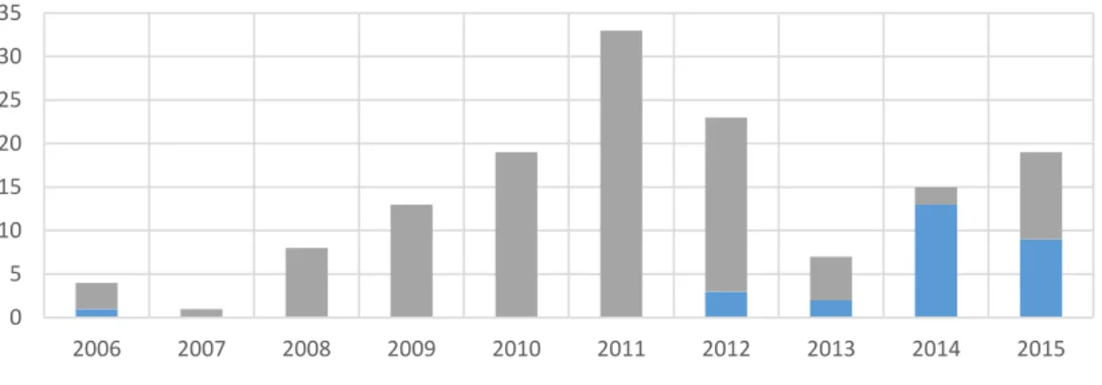
19 S&P was the most active agency with 87 announcements, whereas Moody’s and Fitch had 63 and 58, respectively. Out of these announcements, most of them were downgrades (114) and negative outlooks (65), rather than upgrades (28) and positive outlooks (1). The largest number of announcements took place in 2011 (62), all of them negative (33 downgrades and 29 negative outlooks). In 2011, from the 33 downgrades more than a half concerned to Greece and Portugal.

Figure 3.1. Number and Type of Sovereign Rating Changes per Year

Source: Bloomberg

Two thirds of the upgrades and downgrades are concentrated between 2008 and 2012, i.e. in half of the time studied. Most upgrades took place after 2012, especially in 2014 and 2015.

While Iceland was the country that sooner reacted to the crisis (most downgrades to Icelandic debt occurred in 2008), Greece was the most affected, with the largest number of downgrades (30). Of the 12 countries studied, half of them - Greece, Iceland, Ireland, Italy, Portugal and Spain - represent 89% of the downgrades.

0 5 10 15 20 25 30 35 2006 2007 2008 2009 2010 2011 2012 2013 2014 2015 Upgrade Downgrade

20 3.2. STOCK MARKET RETURNS

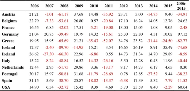
The following table summarizes the annual appreciation (or depreciation, if negative) of each country index value as well as the total appreciation (or depreciation) between 2006 and 2015.

Table 3.2. Index Value Appreciation (in %)

2006 2007 2008 2009 2010 2011 2012 2013 2014 2015 2006-2015 Austria 21.21 -1.01 -61.17 37.68 14.48 -35.92 23.71 3.00 -14.75 9.40 -34.91 Belgium 22.79 -7.33 -53.61 26.80 0.57 -20.84 17.10 16.24 14.05 12.76 24.62 France 16.55 6.85 -42.02 17.51 -5.21 -19.00 13.00 15.05 1.08 9.05 -2.48 Germany 21.04 20.75 -39.49 19.79 14.32 -15.61 25.30 22.80 4.31 10.02 97.12 Greece 19.95 15.95 -65.69 21.21 -35.43 -52.07 34.76 23.52 -31.44 -24.50 -82.77 Iceland 12.37 -2.40 -89.70 -14.95 15.21 3.54 16.65 26.19 8.91 35.49 -74.68 Ireland 26.62 -27.30 -66.30 22.96 -6.86 0.55 14.73 31.34 14.70 29.89 -8.59 Italy 15.22 -8.24 -48.84 16.52 -14.32 -26.16 5.30 12.28 0.43 11.96 -40.44 Netherlands 12.44 2.95 -51.75 29.86 3.36 -13.17 8.17 14.73 6.17 4.63 0.30 Portugal 30.17 15.97 -50.81 31.68 -11.79 -28.69 0.78 12.85 -27.52 9.44 -38.23 Spain 31.15 5.69 -38.70 25.87 -18.82 -13.37 -6.38 17.39 5.32 -7.79 -11.52 USA 14.90 6.34 -32.72 15.42 9.39 4.69 5.70 23.59 8.40 -2.29 60.64 Source: Bloomberg

2008 corresponds to the year in which the highest depreciation is observed. Most indexes lost more than 40% of its value, with the exception of the German (-39.49%), the Spanish (-38.70%) and the American (-32.72%). The Icelandic index was the most affected, having seen its value reduced by almost 90%. In fact, as mentioned before, this is when the country was more penalized in terms of the assessment of its sovereign debt.

Contrary to 2008, 2009 was a year of recovery, except for Iceland that continued depreciating (-14.95%). 2011 is again a year of declines. The exceptions are the Icelandic index, that started recovering in 2010, the Irish, which had a minor increase (+ 0,55%), and the American.

Between 2012 and 2013, only Spain devalued (-6.38% in 2012). It is important to highlight the case of Germany, which increased by more than 20% in both years, and

21 Greece, that recovered part of the loss, after losing more than 30% per year during the previous 2 years.

In 2014, the Portuguese index dropped nearly 28%, and the Austrian, which until then had only fallen in critical years – 2008 and 2011 –, fell almost 15%. The Greek market returned to losses, more than 30% in 2014 and almost 25% in 2015. One should note that there was no downgrade of the sovereign credit rating of Greece in 2014. As a matter of fact, Greek debt was even upgraded by the three agencies. The downgrades just happened in the following year (as well as a couple of upgrades).

In 2015, after experienced a devaluation only in 2008, the American index lost 29.2% of its value. A highlight goes for Iceland, which after its setbacks in 2008 and 2009 has managed to recover, appreciating more than 35% in the last year under review, and Ireland which between 2012 and 2015 achieved gains above 14%.

The final balance, between the years preceding the crisis and the years post crisis, was very positive for the indexes of countries like Germany (+ 97.12%), United States (+ 60.64%) and Belgium (+ 24.62%), but negative for most of them, specially Greece (-82.77%), Iceland (-74.68%), Italy (-40.44%) and Portugal (-38.23%).

22

4. M

4.1.EVENT STUDY

In order to analyze how stock markets respond to changes on sovereign credit ratings, an event study methodology is applied in the current research. This methodology uses financial data to measure the effect of a specific event on a particular variable. In this research, rating announcements denote the event and the effects are measured at the level of stock markets returns.

Following the analysis structure adopted by Campbell, Lo and MacKinley (1996), the first step in an event study is to define the event of interest. After that, the event window must be identified. The event window is the time frame in which the value of the relevant indices for this event will be examined.

Since the appraisal of the sovereign credit ratings announcements impact on stock markets is the main purpose of this paper, the events of interest will be rating announcements, i.e., an upgrade or a downgrade. These are defined as day-zero, because the rating event is considered to occur at time zero (Afonso, Furceri and Gomes, 2012). Regarding the event window, this is usually larger than the specific period of interest and includes at least the day of the announcement. In particular, twelve different windows will be analyzed in this paper, with the aim of identifying market anticipation, immediate reaction and late response to the event of interest.

In order to assess the event’s impact, it is necessary to compute the abnormal returns. An abnormal return can be seen as the difference between the actual return and the normal return4_{. This can be written as}

𝐴𝑅_𝑖𝑡 = 𝑅_𝑖𝑡− 𝐸[𝑅_𝑖𝑡|𝑋_𝑡] (1)

where 𝐴𝑅𝑖𝑡 is the abnormal return on stock market i at day t, 𝑅𝑖𝑡 is the actual return on

stock market i at day t, 𝐸[𝑅_𝑖𝑡] is the normal return on stock market i at day t, and 𝑋𝑡 is

the conditioning information for the normal performance model.

4 _{The logarithmic returns are used, due to their advantages over simple price changes. For further}

23 According to Campbell, Lo and MacKinley (1996, p.151), “there are two common choices for modeling the normal return – the constant-mean-return model where 𝑋_𝑡 is a constant, and the market model where 𝑋𝑡 is the market return”.

Most studies analyse companies’ returns, for which the market model is applicable, but in this paper it is the global market returns that are studied. Therefore, for the current analysis, the constant-mean-return model is the appropriate choice. This model assumes that the mean return of a stock market is constant over time. The constant-mean-return model may be the simplest model, but Brown and Warner (1985) find it to be powerful when it comes to daily returns.

Let 𝜇𝑖 be the mean return for stock market i. Then the constant-mean-return model is

𝑅_𝑖𝑡 = µ_𝑖 + 𝜀_𝑖𝑡 (2)

𝐸[𝜀_𝑖𝑡] = 0 𝑣𝑎𝑟[𝜀_𝑖𝑡] = 𝜎_𝜀2_𝑖

where 𝑅_𝑖𝑡 is the period-t return on stock market i, and 𝜀_𝑖𝑡 is the time period t disturbance term for stock market i, with an expectation of zero and variance

𝜎_𝜀2_{𝑖 =} 1 𝐿 − 2 ∑ (𝑅𝑖𝜏− 𝜇𝑖) 2 𝜏2 𝜏=𝜏1 (3)

L is the length of the estimation window, and 𝜏₁ to 𝜏₂ is the estimation window.

With the selection of a normal performance model, the definition of the estimation window is required. This will be used to estimate the parameters of the model. The most common preference for the estimation window is to use the period prior to the event window. For the current study, the constant-mean-return model parameters will be estimated from 21 to 120 trading days prior to the event, ensuring that the event window, as well as the event of interest, are not included. This will prevent the event, and the days surrounding it, from influencing the normal performance model parameter estimates. After getting the parameter estimates for the normal performance model, the abnormal returns can be computed.

24 Let 𝐴𝑅̂ _𝑖𝜏 be the sample abnormal return of stock market i for period τ, which is included in the event window. Using the constant-mean-return model to measure the normal return, the sample abnormal return is

𝐴𝑅̂_𝑖𝜏 = 𝑅_𝑖𝜏− µ̂_𝑖 (4) where µ̂_𝑖 = 1 𝐿∑ 𝑅𝑖𝜏 𝜏2 𝜏=𝜏1 . (5)

Asymptotically (as L increases5) the variance of the abnormal return is

𝑣𝑎𝑟(𝐴𝑅̂_𝑖𝜏) = 𝜎̂∗_𝜀2_𝑖. (6)

The null hypothesis expresses that the event has no impact on the performance of returns, that is, the abnormal returns have conditional mean and variance zero. Therefore, if there is a test where the null hypothesis is not rejected for all observations, this denotes that the event has no effect on stock markets' returns. This assumption can be employed to any period within the event window, and not just on the event date, and it is also applicable in the case of rejection of the null hypothesis.

The distribution of the sample abnormal return under the null hypothesis is 𝐴𝑅̂_𝑖𝜏~𝑁[0, 𝑣𝑎𝑟(𝐴𝑅̂_𝑖𝜏)].

Since tests with one event observation are useless to draw a feasible conclusion, an aggregation of the abnormal returns must be done. In order to analyze the overall implications for the event of interest, the abnormal returns should be aggregated through time (Cumulative Abnormal Return), across stock markets (Average Abnormal Return), and both (Cumulative Average Abnormal Return).

For this aggregation, the absence of any overlap in the event windows of the involved stock markets is assumed, implying that the abnormal returns and the cumulative abnormal returns are independent across stock markets. For the variance estimators, this assumption is used to set the covariance terms to zero.

25

4.1.1. Cumulative Abnormal Returns

Aggregation of abnormal returns through time, known as Cumulative Abnormal Return (CAR), is firstly considered. The calculation of the CAR is given by the sum of the abnormal returns of a determined stock market i over the event window.

Let 𝐶𝐴𝑅̂_𝑖(𝜏3, 𝜏4) be the sample cumulative abnormal return of stock market i from period

𝜏₃ to 𝜏₄. This can be written as

𝐶𝐴𝑅̂_𝑖(𝜏₃, 𝜏₄) = ∑𝜏4 𝐴𝑅̂_𝑖𝜏

𝜏=𝜏3 (7)

where 𝜏₃ to 𝜏₄ is the event window

Asymptotically (as L increases), the variance of 𝐶𝐴𝑅̂_𝑖(𝜏3, 𝜏4) is

𝑣𝑎𝑟 (𝐶𝐴𝑅̂𝑖(𝜏3, 𝜏4)) = (𝜏4− 𝜏3 + 1)𝜎𝜀𝑖

2 (8)

and its distribution under the null hypothesis is 𝐶𝐴𝑅

̂_{𝑖(𝜏3, 𝜏4)~𝑁 [0, 𝑣𝑎𝑟 (𝐶𝐴𝑅}̂_{𝑖(𝜏3, 𝜏4))].}

4.1.2. Average Abnormal Returns

Aggregation across stock markets, known as Average Abnormal Return (AAR), is then considered. This type of aggregation shows the market average abnormal return for each event period.

Let 𝐴𝐴𝑅̂_𝜏 be the sample average abnormal return for period τ. This can be written as 𝐴𝐴𝑅̂_𝜏 = 1

𝑁∑ 𝐴𝑅̂𝑖𝜏 𝑁

𝑖=1 (9)

where N is the number of stock markets in the sample. Asymptotically (as L increases), the variance of 𝐴𝐴𝑅̂_𝜏 is

𝑣𝑎𝑟(𝐴𝐴𝑅̂_𝜏) = 1 𝑁2∑ 𝜎̂𝜀𝑖 2 𝑁 𝑖=1 (10) 𝑣𝑎𝑟(𝐴𝐴𝑅̂𝜏) = 1 𝑁2∑ 𝑣𝑎𝑟(𝐴𝑅̂𝑖𝜏) 𝑁 𝑖=1 . (11)

26 and its distribution under the null hypothesis is

𝐴𝐴𝑅̂𝜏~𝑁[0, 𝑣𝑎𝑟(𝐴𝐴𝑅̂𝜏)].

4.1.3. Cumulative Average Abnormal Returns

Finally, aggregation across stock markets and through time, known as Cumulative Average Abnormal Return (CAAR), is considered as well in this research. CAARs can be calculated in two different ways: by summing the average abnormal returns from each period of the event window or by averaging the cumulative abnormal returns of each stock market.

Let 𝐶𝐴𝐴𝑅̂ (𝜏₃, 𝜏₄) be the sample cumulative average abnormal return from period 𝜏3 to

𝜏₄. This can be written as

𝐶𝐴𝐴𝑅̂ (𝜏₃, 𝜏₄) = ∑𝜏4 𝐴𝐴𝑅̂_𝑖𝜏 𝜏=𝜏3 (12) or 𝐶𝐴𝐴𝑅̂ (𝜏₃, 𝜏₄) = 1 𝑁∑ 𝐶𝐴𝑅̂𝑖(𝜏3, 𝜏4) 𝑁 𝑖=1 . (13)

Asymptotically (as L increases), the variance of 𝐶𝐴𝐴𝑅̂ (𝜏3, 𝜏4) is

𝑣𝑎𝑟 (𝐶𝐴𝐴𝑅̂ (𝜏₃, 𝜏₄)) = ∑𝜏4 𝑣𝑎𝑟(𝐴𝐴𝑅̂_𝑖𝜏)

𝜏=𝜏3 .

(14) and its distribution under the null hypothesis is

𝐶𝐴𝐴𝑅̂ (𝜏₃, 𝜏₄)~𝑁 [0, 𝑣𝑎𝑟 (𝐶𝐴𝐴𝑅̂ (𝜏₃, 𝜏₄))].

Based on the event methodology, the results need to be tested. For this purpose, a test statistic is usually performed and compared to its assumed distribution under the null hypothesis (Khotari and Warner, 2006).

The null hypothesis is rejected if the test value is in the critical region. However, the null hypothesis is never accepted. Even if the null hypothesis is not reject, it does not mean that it should be accepted. If the test value is in the critical region, there is statistical evidence to doubt about the truth of the null hypothesis. This “doubt” is called significance level and it is usually between 0.01 and 0.05. The critical value, from which

27 the absolute test value is rejected, depends on the significance level: 2.575 and 1.96, respectively for a 5% and 1% significance level.

Using the “basic approach” (Campbell, Lo and MacKinley, 1996), we perform two alternative statistical tests of hypothesis: 1) Average Abnormal Return at period τ is equal to zero; 2) Cumulative Average Abnormal Return from 𝜏₃ to 𝜏₄ is equal to zero. These tests are important to understand if there was a response (or even an anticipation) to the sovereign credit rating changes, or, on the contrary, there was no reaction from the stock markets.

Regarding the Average Abnormal Returns, the null hypothesis can be tested using 𝜃₁ = 𝐴𝐴𝑅̂𝜏

√𝑣𝑎𝑟(𝐴𝐴𝑅̂_𝜏).

(15)

In what concerns the Cumulative Average Abnormal Returns, the null hypothesis can be tested using

𝜃2 =

𝐶𝐴𝐴𝑅̂ (𝜏3,𝜏4)

√𝑣𝑎𝑟(𝐶𝐴𝐴𝑅̂ (𝜏3,𝜏4))

. (16)

28

5. E

R

The presentation of the empirical results is as follows. The differences on the outcomes between upgrades and downgrades are discussed initially6. Then, the impact of downgrades is analysed in more detail, first, by rating agency, and, second, by period of time. Finally, the cross-country contagion of downgrades is also examined.

5.1. DOWNGRADES VS UPGRADES

Regarding upgrades and downgrades, there are very distinct conclusions. In both cases we find no impact on the day before the event. However, on the day of the event and on the day after there are significant abnormal returns with respect to upgrades and downgrades, respectively.

As can be seen from table 5.1, while upgrades have a significant abnormal average return on day 1 – the day after the event –, downgrades have it immediately on the day of the event. This may be due to two situations: either upgrades are mostly done when the stock markets are already closed, leading the reaction to the next day, or there is a more instantaneous reaction of markets to downgrades.

When analysing the days preceding the event, it can be concluded that, both in the case of upgrades and downgrades, there is no suggestion of anticipation. The only days with significant AAR before the event are from upgrades and are negative. This result does not confirm the one from Norden and Weber (2004), that indicates that both bond and stock markets anticipate rating announcements, particularly, downgrades.

6 _{Outlooks are not included, since the main goal of this paper is to investigate the impact of credit rating}

29

Table 5.1. Average Abnormal Returns and respective t-test value by type of

announcement Trading Day Upgrade N=28 Downgrade N=103

AAR (%) t-test AAR (%) t-test -20 -0.31 -1.05 -0.01 -0.06 -19 -0.70 -2.37* -0.19 -0.85 -18 0.01 0.04 -0.09 -0.40 -17 0.02 0.06 0.11 0.48 -16 0.56 1.89 0.23 1.03 -15 -0.04 -0.15 0.30 1.38 -14 -0.24 -0.82 -0.15 -0.71 -13 -0.19 -0.65 0.05 0.22 -12 0.13 0.45 0.14 0.64 -11 -0.67 -2.27* 0.04 0.20 -10 -0.49 -1.64 0.01 0.03 -9 -0.11 -0.37 0.21 0.96 -8 0.04 0.12 0.10 0.46 -7 0.32 1.09 -0.12 -0.56 -6 -0.14 -0.47 -0.05 -0.22 -5 0.35 1.17 -0.01 -0.05 -4 0.13 0.43 0.07 0.30 -3 0.12 0.40 0.22 1.01 -2 0.05 0.17 0.16 0.76 -1 0.02 0.06 -0.15 -0.71 0 -0.10 -0.35 -0.76 -3.50** 1 0.88 2.99** 0.09 0.40 2 -0.40 -1.37 0.23 1.06 3 -0.29 -1.00 -0.62 -2.87** 4 -0.85 -2.87** 0.42 1.92 5 -0.18 -0.62 -0.97 -4.46** 6 -0.19 -0.63 -0.09 -0.40 7 -0.20 -0.68 0.10 0.48 8 0.01 0.02 0.30 1.38 9 -0.23 -0.79 -0.95 -4.38** 10 -0.19 -0.64 -0.98 -4.51** 11 -0.11 -0.38 0.06 0.29 12 0.10 0.33 0.08 0.38 13 0.04 0.13 -0.19 -0.85 14 -0.12 -0.42 0.32 1.47 15 -0.23 -0.76 0.25 1.15 16 -0.53 -1.80 -0.15 -0.67 17 0.15 0.51 -0.18 -0.82 18 0.55 1.86 -0.03 -0.14 19 0.13 0.45 0.01 0.05 20 -0.54 -1.84 -0.40 -1.84

Bold t-tests represent statistically significant rejections of the null hypothesis: * with a 5% significance level; ** with a 1% significance level.

30 Through the analysis of different windows, it is possible to obtain important conclusions about the surrounding days to the day of the event. In this context, twelve event windows with different lengths are created (table 5.2). They are divided into 4 groups and each one has three event windows: one with the day(s) before and after, one with the day(s) before and one with the day(s) after the event. All groups include the day of the announcement of downgrades or upgrades.

Table 5.2. Cumulative Average Abnormal Returns and respective t-test value by type of

announcement Trading Day Upgrade N=28 Downgrade N=103

CAAR (%) t-test CAAR (%) t-test [-1, 1] 0.80 1.55 -0.83 -2.20* [-1, 0] -0.09 -0.21 -0.92 -2.98** [0, 1] 0.78 1.86 -0.68 -2.19* [-5, 5] -0.30 -0.30 -1.34 -1.85 [-5, 0] 0.55 0.76 -0.48 -0.90 [0, 5] -0.95 -1.31 -1.62 -3.04** [-10, 10] -1.47 -1.09 -2.81 -2.82** [-10, 0] 0.18 0.18 -0.33 -0.46 [0, 10] -1.75 -1.79 -3.24 -4.48** [-20, 20] -3.48 -1.84 -2.60 -1.87 [-20, 0] -1.26 -0.93 0.09 0.09 [0, 20] -2.32 -1.71 -3.45 -3.46**

Bold t-tests represent statistically significant rejections of the null hypothesis: * with a 5% significance level; ** with a 1% significance level.

Analysing table 5.2, one might conclude that, despite the significant abnormal return of 0.88% on day 1 (table 5.1), no event window of upgrades has significant CAAR. Concerning downgrades, there are significant negative cumulative average abnormal returns in the days following the announcement, with the null hypothesis being rejected in all corresponding windows. The 10-day window is the one with the greater critical value (t value equal to -4.48), negatively influenced not only by the effects on the day of the event, but also by the negative effects observed on the 3rd, 5th, 9th and 10th days (table 5.1). In contrast, we reject H0 in all windows that include only the previous days – with

31 the exception of the [-1, 0] trading range, that is strongly influenced by day 0. This could mean that the market does not anticipate – such as Norden and Weber (2004) sustain –, but instead react to the announcements, in line with Kaminsky and Schmuker (1999). Figure 5.1 allows us to examine the trend of both types of announcements along the event window [-20, 20].

Figure 5.1. Cumulative Average Abnormal Returns by Type of Announcement

As can be seen both in figure 5.1 and in table 5.2, the CAAR in the event window [-20, 20] for both types of event is negative, but not significant, that is, we do not reject the null hypothesis.

The trend – before, for downgrades, and after the event, for upgrades – is counterintuitive. For upgrades, contrary to what is expected – since they transmit a positive market information – there is a decrease on CAAR after the announcement. In the case of downgrades, the CAAR on the day of the event is positive, showing no anticipation and even a positive expectation of the market. However, no precise conclusions can be taken about this, since results are not statistically significant.

Nevertheless, analysing only the 20 days after the event window, the cumulative average abnormal returns of the downgrades are quite significant. This confirms the conclusions

-5 -4 -3 -2 -1 0 1 2 -20 -15 -10 -5 0 5 10 15 20 CA A R (% ) Trading Day Upgrade Downgrade

32 of previous literature: significant negative impact of downgrades and no substantial effect of upgrades (see, for instance, Faff et al., 2001; Dichev and Piotroski, 2001; Ferreira and Gama, 2007).

5.2. DOWNGRADES BY AGENCY

Some studies point to different market reactions to a downgrade according to the rating agency making the announcement. This suggests that the agencies influence investors in a different way, i.e., announcements by some agencies exert a higher influence on market prices than others. However, there is no agreement on which is the agency providing the most effective announcements.

For that reason, the average abnormal returns and the cumulative average abnormal returns by rating agency are studied in order to reach a conclusion.

Table 5.3. Average Abnormal Returns and respective t-test value by agency

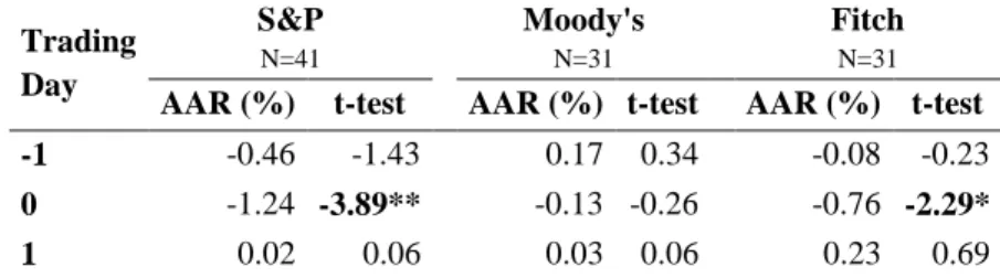
Trading Day S&P N=41 Moody's N=31 Fitch N=31

AAR (%) t-test AAR (%) t-test AAR (%) t-test -1 -0.46 -1.43 0.17 0.34 -0.08 -0.23

0 -1.24 -3.89** -0.13 -0.26 -0.76 -2.29*

1 0.02 0.06 0.03 0.06 0.23 0.69

Bold t-tests represent statistically significant rejections of the null hypothesis: * with a 5% significance level; ** with a 1% significance level.

Complete table can be seen on appendix 8

When examining the AAR in table 5.3, one can conclude that announcements by S&P and Fitch are significant on the day of the announcement, leading to the rejection of the null hypothesis with a 1% and a 5% level of significance, respectively. In contrast, the AAR from Moody's, though negative, seems to have no impact on markets.

33

Table 5.4. Cumulative Average Abnormal Returns and respective t-test value by agency

Trading Day S&P N=41 Moody's N=31 Fitch N=31

CAAR (%) t-test CAAR (%) t-test CAAR (%) t-test [-1, 1] -1.68 -3.04** 0.07 0.08 -0.61 -1.05 [-1, 0] -1.70 -3.76** 0.04 0.06 -0.84 -1.78 [0, 1] -1.22 -2.71** -0.10 -0.14 -0.53 -1.13 [-5, 5] -4.22 -3.98** 0.85 0.53 0.29 0.26 [-5, 0] -1.59 -2.03* 1.17 0.98 -0.65 -0.80 [0, 5] -3.87 -4.95** -0.44 -0.37 0.17 0.21 [-10, 10] -5.61 -3.83** 0.29 0.13 -2.20 -1.44 [-10, 0] -1.61 -1.52 1.22 0.76 -0.20 -0.18 [0, 10] -5.24 -4.95** -1.06 -0.66 -2.76 -2.50* [-20, 20] -4.26 -2.08* 0.42 0.14 -3.43 -1.61 [-20, 0] -0.02 -0.01 1.15 0.52 -0.85 -0.55 [0, 20] -5.48 -3.75** -0.86 -0.39 -3.35 -2.19*

Bold t-tests represent statistically significant rejections of the null hypothesis: * with a 5% significance level; ** with a 1% significance level

As shown in table 5.4, the announcements of S&P are the ones that have more impact on stock markets. This supports previous literature, such as Reisen and von Maltzan (1999), and Brooks et. al (2001). One possible reason is the fact that the S&P rating changes precede the ones from the other agencies (see Gande and Parsley, 2005), leading to a lower impact of the latter, once the stocks already reflected the deterioration of the sovereign debt creditworthiness. When analysing the six countries with the largest number of downgrades of the sample (Greece, Iceland, Ireland, Italy, Portugal and Spain), it is, in fact, S&P, followed by Fitch, the agencies that generally downgrade earlier sovereign issuers (see appendix 6).

By examining the different event windows of S&P, on table 5.4, one comes to the conclusion that markets do not anticipate, but react to its downgrades. Despite the event windows [-1, 1] and [-5, 5] being significant, it is not correct to affirm that there is anticipation, since their critical value, calculated without including the day of the event, is -1.43 and -0.44, respectively. This can also be seen on the following figure 5.2. This figure allows us to examine the trend of the three credit rating agencies along the event window [-20, 20] after a downgrade.