UNIVERSIDADE T ´
ECNICA DE LISBOA
INSTITUTO SUPERIOR DE ECONOMIA E GEST ˜
AO
Mestrado em: Econometria Aplicada e Previs˜ao
Multivariate Filtering with Common Factors
Ana Regina Nunes Pereira
Orientac¸˜ao: Prof. Doutor Jo˜ao Valle e Azevedo
J´uri:
Presidente: Prof. Doutor Artur Carlos Barros da Silva Lopes
Vogais:
Prof. Doutor Paulo Manuel Marques Rodrigues Prof. Doutor Jo˜ao Carlos Henriques da Costa Nicolau Prof. Doutor Jo˜ao Valle e Azevedo
Abstract
This study discusses four commonly used optimal approximations to the infinite order moving average filter that ideally extracts from a time series fluctuations within a specified range of periodicities. Based on our findings, we use two of those approximations in the estimation of two macroeconomic signals: business cycle fluctuations and medium to long run component of output growth rate. This study dis-tinguishes itself from related literature by showing how to successfully incorporate in the multivariate band-pass approximations factors estimated from a large panel of time series.
As illustration, we apply these approximations to U.S. data. We evaluate the real-time performance of the indicators and provide forecasting comparisons. The results suggest that the multivariate indica-tor outperforms the competing univariate indicaindica-tor across all different settings considered. Moreover, multivariate methods that target smooth growth are useful to forecast quarterly GDP growth rate at short-term and to forecast yearly GDP growth.
Resumo
Este estudo discute quatro aproxima¸c˜oes ´optimas ao filtro de m´edias m´oveis infinitas que idealmente isola de uma s´erie temporal flutua¸c˜oes compreendidas num determinado intervalo de periodicidades. De acordo com as nossas conclus˜oes, utilizamos duas dessas aproxima¸c˜oes na estima¸c˜ao de dois sinais macroecon´omicos: flutua¸c˜oes de ciclo econ´omico no produto e a componente de m´edio e longo prazo da taxa de crescimento do produto. Este estudo distingue-se da literatura corrente ao mostrar como integrar nas aproxima¸c˜oes do filtro banda multivariado factores estimados a partir de um largo painel de s´eries temporais.
Como ilustra¸c˜ao, aplicamos estas aproxima¸c˜oes a dados dos E.U.A.. Avaliamos o desempenho dos in-dicadores em tempo real e apresentamos compara¸c˜oes em termos de previs˜ao. Os resultados sugerem que o indicador multivariado tem um desempenho claramente superior ao do indicador univariado em todos os cen´arios considerados. Adicionalmente, os m´etodos multivariados que aproximam o crescimento alisado s˜ao ´uteis na previs˜ao da taxa de crescimento trimestral do PIB a curto prazo e para previs˜ao do crescimento anual do PIB.
Contents
1 Introduction 1
2 Setting the problem 5
2.1 Optimal approximations . . . 11
2.1.1 The Baxter and King approximation . . . 12
2.1.2 The Christiano and Fitzgerald approximation . . . 15
2.1.3 The Multivariate approximation . . . 21
2.1.4 The Hodrick and Prescott filter . . . 25
2.2 Comparison . . . 28
3 Estimation of moments and factor models 37 3.1 Estimation of second order moments . . . 37
3.2 Multivariate information . . . 40
3.2.1 Factor model . . . 40
3.2.2 Estimation of the factors . . . 42
3.2.3 Estimation of the number of factors . . . 45
4 Real Data Application 47 4.1 Dataset . . . 47
4.2 Covariates used in the multivariate approximation . . . 50
4.3 Number and estimation of the factors . . . 50
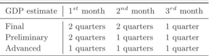
4.4 Release delays . . . 51
4.5 Different types of estimates . . . 53
4.6 Performance of the indicators . . . 53
4.6.1 Business cycle fluctuations . . . 55
4.6.2 Smooth growth . . . 61
4.7 Forecast performance . . . 65
4.7.1 Quarterly growth . . . 65
4.7.2 Yearly growth . . . 68
List of Figures
1 Time domain representation of the weights of the ideal filters. . . 7
2 Approximations to the business cycle fluctuations of U.S. real GDP using alternative filtering techniques. . . 29
3 Panel A. Gain function of the ideal low pass filter against the gain function of the Hodrick and Prescott growth filter; Panel B: Gain function of the ideal high pass filter against the gain function of the Hodrick and Prescott cyclical filter. . . 30
4 Gain function of the ideal band-pass filter against the gain functions of the Hodrick and Prescott cyclical filter and the Baxter and King filter.. . . 31
5 Gain function of the ideal band-pass filter against the gain function of the Baxter and King filter for different truncation values. . . 32
6 Approximation to the business cycle fluctuations of U.S. real GDP using the Baxter and King filter. . . 33
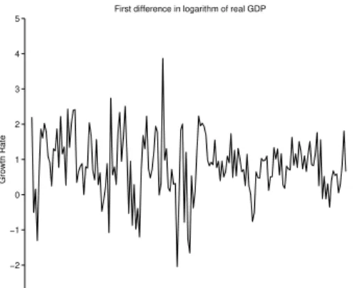
7 Logarithm of real GDP and of the first difference of the logarithm of real GDP. . . 47
8 Sample autocorrelation function of the logarithm of real GDP and of the first difference of the logarithm of real GDP. . . 48
9 Business cycle fluctuations: final,real-time andtoday onwardsestimates . . . 59
10 Evaluation of the approximations to business cycle fluctuations: correlation, noise to signal ratio and sign concordance. . . 60
11 Smooth growth: final,real-time andtoday onwards estimates. . . 64
12 Evaluation of the approximations to smooth growth: correlation and noise to signal ratio 65 13 U.S. yearly real GDP growth rate: actual and implicit. . . 68
14 Yearly GDP growth rate and real-time forecasts made at the end of March, June, Septem-ber and DecemSeptem-ber. . . 72
15 Left panel displays a simulated AR(1) model and right panel displays the population spectrum for an AR(1) model. . . 7
16 Population spectrum for an MA(1) model. Panel A.θ= 5; Panel B.θ=−2. . . 8
17 Gain and phase shift. . . 11
18 Squared gain of the first difference filter. . . 20
List of Tables
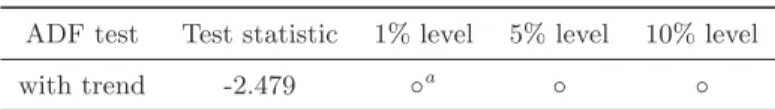
1 Baxter and King’s objectives. . . 12 2 Results of ADF test on logarithm of real GDP. . . 49 3 Release delays of U.S. GDP estimates by month of the quarter.. . . 52 4 Evaluation statistics for the approximations to business cycle fluctuations in the U.S in
the third month of the quarter. . . 56 5 Evaluation statistics for the approximation to business cycle fluctuations in the U.S. in
every month of the quarter. . . 58 6 Evaluation statistics for the approximations to smooth growth in the U.S. in the third
month of the quarter. . . 61 7 Evaluation statistics for the approximations to smooth growth in the U.S. in every month
of the quarter. . . 63 8 Ratio of the mean squared error of the forecasts of each method to the mean squared
error of an univariate regression forecast (quarterly growth rate). . . 67 9 Ratio of the mean squared error of the forecasts of each method to the mean squared
1
Introduction
A main concern of macroeconomic analysts, policy makers and others lies in tracking, in real time, the state of the economy. So, they focus attention on signals that aim at summarizing information embedded in the time series movements of major macroeconomic aggregates.
The idea that an individual time series can be seen as the sum of multiple components driven by different kinds of shocks follows from Persons’ (1919) work. Ever since several methods have been proposed in the literature to measure those different components; in particular the trend and cyclical component. Methods can be divided into two groups: economic-based models and statistical-based models. The first group uses economic theory to explain the mechanism of fluc-tuations while the second group uses purely statistical assumptions to identify the components. A brief survey of the literature indicates as references for a discussion of economic-based models Singleton (1988), King et al. (1988, 1991), Blanchard and Quah (1989) and Cochrane (1994). Alternatively, statistical-based models include deterministic detrending, first differences, Bev-eridge and Nelson’s (1981) decomposition, unobserved components models, filtering techniques, Stock and Watson’s (1998) index models or Altissimo et al.’s (2008) projection problem.
In this study the main objective will be to construct a real time indicator for two specific macroeconomic signals: business cycle fluctuations of aggregate output and smooth component of output growth (henceforth smooth growth). We will use a filtering approach to directly obtain such signals, which amounts to apply to the series of interest a filter specifically designed to isolate only the fluctuations within a pre-specified range of periodicities. Unlike most methods, filtering techniques clearly permit to achieve an explicit separation between components and additionally provide a simple way to accomplish such task. The downside follows from the statistical nature of this approach that compromises the interpretation of the extracted components from an economic point of view.
important information to assess the direction of the economy. Moreover, we view forecasts of the smooth growth indicator as being useful to forecast GDP growth itself because the possibly unpredictable short-run oscillations, approximated by conventional models, have been eliminated. Our empirical application provides important insights regarding this matter.
Both signals can be obtained by applying an infinite order moving average filter to the series of interest. However, this procedure implies infinite data and thus an approximate filter is required for empirical purposes. According to an optimization criterion, good approximations to the ideal infinite sample filter are proposed by Hodrick and Prescott (1997), Baxter and King (1999) and Christiano and Fitzgerald (2003) in an univariate context and by Valle e Azevedo (2007) in a multivariate context. In the first part of this study we analyze in detail the properties of each of these approximations and discuss which ones are suitable for real time analysis. We conclude, given our objective, that Hodrick and Prescott’s filter as well as Baxter and King’s filter detain undesirable features. Therefore, only the two remaining approximations from those mentioned earlier can be used to construct a real-time indicator.
The second part of this work provides an empirical application of the optimal filter suggested by Christiano and Fitzgerald and of the optimal filter suggested by Valle e Azevedo to U.S. quarterly GDP or GDP growth rate, depending on the signal. The univariate filter is used as a benchmark filter for comparisons and the multivariate approximation is adopted as our proposed indicator. The multivariate optimal filter does not only exploit the information in a single time series but also that in a large panel of monthly economic variables. To compress this additional information, the panel is assumed to be described by a dynamic factor model, as originally developed by Geweke (1977) and Sargent and Sims (1977). To be specific, each variable of the panel is assumed to be described by a few number of common factors plus an idiosyncratic error. These factors are unobservable variables and therefore estimated using either principal components as in Stock and Watson (2002a, 2002b) or generalized principal components as in Forni et al. (2005). Accordingly, we compare the two methods of approximating the factor space. The extracted factors are then incorporated as covariates in the multivariate approximation of the signals of interest.
approach that combines information derived from a large panel of time series (reduced by estima-tion of common factors). Moreover, our multivariate approach can be used in any similar signal extraction problem since it can easily be adapted to optimally approximate any other signal of interest or equivalently to extract any other range of periodicities.
To simulate a true real time exercise both signals are defined on the GDP of the current quarter and the release delays of all the variables involved is taken into account. This implies that our real activity indicators will be timely and that our method is flexible enough to easily produce real time estimates. Furthermore, the elimination of fluctuations with low periodicities implies that the indicators will display little short-run oscillations, thereby giving a clear picture of current cyclical and growth prospects. Finally, due to the monthly frequency of the variables of the panel we are able to obtain an update of the multivariate indicator each month and not just at a quarterly frequency as for the univariate filter. All these features stress the advantages inherent to our method.
Our findings reveal that the multivariate indicator outperforms the competing univariate indicator across all settings considered in all months of the year. These settings include variations in the estimation procedure of factors and second order moments. In detail, the best performing indicator for both signals is the multivariate filter using two monthly factors and moments derived from a parametric estimator. We conclude that exploiting information in other variables other than real GDP is helpful in mitigating the approximations errors arising from missing data.
In addition, as a by-product we use the best performing multivariate filter for forecasting quarterly and yearly output growth rates. This exercise gives important insights on whether it is more relevant, for forecasting purposes, to target a smooth version of a time series or instead the original time series containing the irregular oscillations. We found that multivariate methods that target smooth growth are useful for short-term forecast of quarterly growth rates and that at long horizons all methods seem useless for forecasting purposes. These results support the findings of Runstler et al. (2008) and Reichlin et al. (2008). In terms of forecasting the yearly growth rate we report a surprising accuracy in the multivariate forecasts that are derived from approximations to smooth growth, even at the end of the first quarter of the year, where the task is rather demanding.
2
Setting the problem
In this section we define precisely the signals (or components) that we aim to isolate from a time series and review some of the methods available to optimally approximate them.
Our objective is to obtain two distinct macroeconomic signals: business cycle fluctuations and the medium to long run component of the output growth rate. To this effect, we will center our attention on real Gross Domestic Product (GDP) since it is the best available proxy of the aggregate economic activity. The business cycle fluctuations will be extracted from the logarithm of GDP, denoted byyt, while the medium to long run component will be extracted from the GDP growth rate, denoted by ∆yt= (1−L)ytwhere Lis the lag operator.
In a frequency domain perspective1, business cycle fluctuations can be identified as those fluctuations with a specified range of periodicities (see Baxter and King, 1999) in the (pseudo-) spectrum ofyt2. Following Burns and Mitchell (1946), the range limits should be set to 6 and 32 quarters, meaning that the cyclical component of GDP is composed of all cycles with period no less than 6 quarters and no more than 32 quarters. This definition of business cycle fluctuations is completely arbitrary in the sense that it is always possible to extract fluctuations in any other range of periodicities that one might understand as cyclical movements. Furthermore, we argue that the definition of the different components of a time series, in particular that of business cycle fluctuations, is model-dependent. For now we adopt this widely used definition but we will contrast it with others, in particular with the Hodrick and Prescott filter (see below). The medium to long run component of GDP growth rate (henceforth smooth growth) is defined as the output growth cleaned of fluctuations with period less than one year (4 quarters), as in Altissimo et al. (2008)3. Note that this signal can be seen as the trend-cycle component of the GDP growth
rate, which excludes variability of short duration. Accordingly, it will vary smoothly over time and it is precisely this characteristic that makes this signal an interesting predictor of GDP growth. This last idea will be explored in section 4. Moreover, both signals exclude irregular and seasonal variation by eliminating all fluctuations with period less than 6 quarters in the case of business cycle fluctuations and 4 quarters in the case of smooth growth. This reduces the
1For more details on the frequency domain approach see Appendix A. 2The spectrum is only well defined ify
tis a stationary process. Given that GDP may contain a unit root we
define instead the pseudo-spectrum, which is not well defined at frequency zero.
3Altissimo et al. (2008) define this signal to construct the new EuroCoin indicator, which is a coincident
need to account for GDP data revisions if these have most of its power concentrated in the high frequencies. Nevertheless, we still have to account for other types of revisions.
We now turn to the particular question of how to obtain these signals. It is well-known that any arbitrary signal can be extracted by applying a two-sided infinite order moving average to the series of interest (zt). As presented in more detail in Appendix B the application of such a linear filter to a covariance stationary time serieszt results in
xt=
∞
X
j=−∞
Bjzt−j=B(L)zt
wherextdenotes the component to be extracted from zt,B(L) =P
∞
j=−∞BjLj where Lis the lag operator and ©Bj:j = 0,+−1,+−2, . . .
ª
are weights verifying P∞j=−∞|Bj| < ∞ (absolutely summable).
In order to isolate only specific movements, we will have to chose a particular design for the weight sequence, which is better handled via frequency domain analysis. In this perspective, the focus is on the spectral density function (or spectrum) which decomposes the time series fluctuations into orthogonal frequencies. Each component of a time series can be distinguished from others by the different amount of time it requires to complete a whole cycle, or equivalently, we may say that each component is connected with specific periodicities. In turn, these latter periodicities (p) relate to frequencies (ω) throughp= 2π
ω, suggesting that each component can be indistinctly identified either by their range of periodicities or range of frequencies. Under the assumption thatzt is a covariance stationary process with absolutely summable autocovariance functionγz(k), k= 0,+−1,+−2, . . . ,the spectrum of the filtered series,Sx(ω), is given by
Sx(ω) =
¯
¯B¡e−iω¢¯¯2S
z(ω), −π≤ω≤π (1)
whereB¡e−iω¢=P∞
j=−∞Bje−iωj is the frequency response function (or the Fourier transform) of the linear filterB(L) andSz(ω) = 21π
P∞
h=−∞γz(h)e−iωh is the spectrum ofzt. The function
¯
¯B¡e−iω¢¯¯2 in equation (1) is known as transfer function (or square gain function) and works as a weighting sequence of the spectrum of the series to be filtered. Given a particular frequency ¯ω, if¯¯B¡e−iω¯¢¯¯2>1 (or <1) then the fluctuations ofz
t with periodicity 2ω¯π will pass to xt with
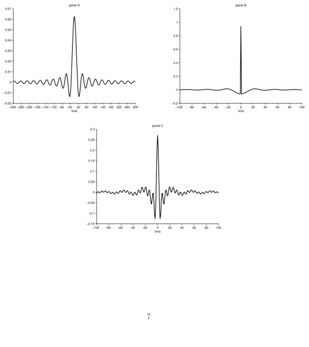
ofztwith periodicity 2ω¯π will be completely removed (exactly preserved) fromxt. Given the role of the gain function in the spectrum of the filtered series and the correspondence of frequencies to periodicities it is straightforward to construct a linear filter that exactly preserves fluctuations within specific periodicities and that completely eliminates all the other undesirable fluctuations. This type of linear filters are referred to as ideal filters and a discussion of their characteristics is provided in Appendix B. Figure 1 shows the ideal behavior of the infinite moving average weights (in the time domain) when the goal is to extract a component related to low frequencies (panel A), high frequencies (panel B) or intermediate frequencies (panel C).
Figure 1: Time domain representation of the weights of an ideal low pass filter (panel A), an ideal high pass filter (panel B) and an ideal band-pass filter (panel C).
−300 −260 −220 −180 −140 −100 −60 −20 20 60 100 140 180 220 260 300 −0.02
−0.01 0 0.01 0.02 0.03 0.04 0.05 0.06 0.07
time panel A
−100 −80 −60 −40 −20 0 20 40 60 80 100 −0.2
0 0.2 0.4 0.6 0.8 1 1.2
time panel B
−100 −80 −60 −40 −20 0 20 40 60 80 100 −0.15
−0.1 −0.05 0 0.05 0.1 0.15 0.2 0.25 0.3
Reviewing, to extract a particular signal we have to first specify its characteristics in terms of frequencies or periodicities and then apply the infinite order moving average filter with the proper weights to the series of interest. Obviously, in empirical studies some finite version of those filters is used instead, but this will be subject for discussion in the next subsection. For now we focus on translating the previous ideas to the specified signals.
Define the following decomposition ofyt and ∆yt:
yt=BC(L)yt+ (1−BC(L))yt (2)
∆yt=SG(L)∆yt+ (1−SG(L))∆yt (3)
where the logarithm of GDP and the GDP growth rate are regarded as a sum of two components; one with power only at the frequencies of interest, namelyBC(L)ytandSG(L)∆yt, and a second with power outside those frequencies. Business cycle fluctuations and smooth growth rates are obtained by applying to yt and ∆yt, respectively, a infinite, symmetric and two-sided filter as follows
BC(L)yt =
∞
X
j=−∞
BCjLjyt
SG(L)∆yt =
∞
X
j=−∞
SGjLj∆yt
with
BC0=ωuπ−ωl, BCj= sin(ωuj)πj−sin(ωlj), |j| ≥1 withωl= 232π andωu= 26π (4)
SG0=
ωu
π , SGj =
sin(ωuj)
πj , |j| ≥1 withωu= 2π
4
whereωlis the lowest frequency andωuis the highest frequency of the frequency band of interest. Accordingly the spectra of the desired components are given by
SBC(ω) =
¯
¯BC¡e−iω¢¯¯2S
y(ω), −π≤ω≤π ω6= 0 (5)
SSG(ω) =
¯
¯SG¡e−iω¢¯¯2S
∆y(ω), −π≤ω≤π
where ω is a frequency defined in radians, BC¡e−iω¢ = P∞
response function of the linear filter BC(L), SG¡e−iω¢ = P∞
j=−∞SGje−iωj is the frequency response function of the linear filter SG(L), Sy(ω) is the pseudo-spectrum of real GDP and S∆y(ω) the spectrum of GDP growth rate. Remembering the equivalence between periodicities and frequencies as well as the signals’ exact definitions it is evident what will be the designs of the squared gain functions. Extracting business cycle fluctuations amounts to isolate the interval of frequencies [2π/32; 2π/6] from the pseudo-spectrum ofytwhereas extracting the smooth growth amounts to isolate all frequencies lower than 2π/4 from the spectrum of ∆yt. Thus, in the first case the filter must retain without distortion fluctuations in a time series between a lower and upper bound frequency and remove completely all variations outside this range of frequencies. In the case of the smooth growth component the filter must eliminate the high frequency movements and preserve the frequencies connected to long and medium term fluctuations.
As a result, the filterBC(L) will be an ideal band-pass filter and so its gain function is
¯
¯BC¡e−iω¢¯¯2=
1, ωl≤ |ω| ≤ωu 0, elsewhere
(6)
with ωl = 232π and ωu = 26π denoting the lower and upper frequencies. The linear filterBC(L) removes unit roots becauseBC(1) = 0. So, the signalxt=BC(L)ytis stationary, even whenyt is integrated of order 1, and contains only fluctuations with frequencies in the specified range. In the presence of a unit root process, like real GDP usually is, one must define the spectrum of an integrated series in order to interpret the relation in (5) as usual. The pseudo-spectrum of an integrated series is routinely defined as the limit of the spectrum of a stationary process when the smallest autoregressive roots converge to 1 (see Harvey, 1993, Den Haan and Sumner, 2004, Young et al., 1999). Accordingly, ifytfollows and ARIMA(p,1,q) process its pseudo-spectrum is
Sy(ω) = σǫ2 2π
ψ(e−iω)ψ(eiω) (1−e−iω)(1−eiω)
where yt satisfies (1−L)yt =ψ(L)ǫt and ǫt is a white noise sequence with varianceσǫ2. This function is well defined for all frequencies except atω= 0. In any case, we conclude that equation (5) holds by definition ifSy(ω) is defined as the pseudo-spectrum. Whenω∈[ωl;ωh]⊆]0;π] the pseudo-spectrum is well defined andBC(e−iω) = 1 soS
BC(e−iω) = 0 by definition andS
x(ω) = 0. Finally, if the pseudo-spectrum is not well defined (or ω = 0) we conclude that Sx(0) = 0. This follows from two observations: first BC(L) can be factored asBC(L) = (1−L)2BC
∗∗(L) = (1−L)BC∗(L) because the ideal band-pass filter
removes unit roots and this implies thatBC∗(1) = 0 and secondxt=BC(L)yt=BC∗(L)(1−
L)yt=BC∗(L)ztbut ztis stationary and its spectrum is well defined for all frequencies. Some researchers however argue that (5) does not hold because unit root processes theoretically do not have a spectral density function. Follows that it is a meaningless discussion if the focus is on the signal because, regardless of the interpretation given to Sy(ω), the ideal band-pass filter will still isolate a component with fluctuations within the specified range of periodicities. However, the spectrum ofxtoften will exhibit a sharp peak at the lowest frequency of the band of interest and some researchers wrongly associate that pattern with the presence of spurious cycles. Clearly that is not a consequence of filtering a unit root process as argued by Cogley and Nason (1995) and others because a similar behavior arises when filtering highly persistent but stationary processes (see Pedersen 2001).
For the smooth growth case we set up an ideal low pass filter and so the gain function of SG(L) follows
¯
¯SG¡e−iω¢¯¯2=
1, |ω| ≤ωu 0, elsewhere
withωu= 24π denoting the threshold frequency.
At this point it is clear that the extraction of the signals entails a infinite number of weights. In such case an approximation is required. The usual approach is to obtain an optimal approxi-mation, in other words, the minimum mean square error (MSE) estimate of the signal. In detail, this involves specifying the mean square error as loss function
L=E[(xt−xˆt)2]
approximation. In frequency domain representation we have4 ˜ L(ω) = Z π −π ¯ ¯
¯B¡e−iω¢−Bˆ¡e−iω¢¯¯
¯
2
Sy(ω)dω
where B(z) denotes the frequency response function of the ideal filter, ˆB(z) denotes the fre-quency response function of the approximate filter andSy(ω) the spectrum (or pseudo-spectrum) ofyt. To obtain an approximate filter with optimal weights the following optimization problem is solved
M in
{Bˆj}p j=−f
˜
L(ω) = M in
{Bˆj}p j=−f
Z π
−π
¯ ¯
¯B¡e−iω¢−Bˆ¡e−iω¢¯¯
¯
2
Sy(ω)dω. (7)
The objective function equals the square modulus of the difference between the frequency domain representation of the ideal filter and the frequency domain representation of the approximate filter, weighted at each frequency by the spectrum of the time series to be filtered. The optimal weights will depend on the ideal weights and on the properties of the series to be filtered due to the presence of the spectrum in the loss function. However, as the true times series representation is unknown the spectrum is in practice replaced by its empirical counterpart (see below for a discussion of this point).
2.1
Optimal approximations
This section analyzes in some detail four suggested approximations to business cycle fluctuations, i.e., solutions to the minimization problem in equation (7) withB¡e−iω¢given in equation (6). An approximation to smooth growth is obtained by adapting the following approximate filters to a different frequency band and to the case of filtering a stationary time series.
4To obtain the frequency domain representation of the loss function definex
t= Γ(L)ytwith Γ(L) =B(L)−
ˆ
B(L). In Appendix A we show that the spectrum ofxt is
Sx(ω) =
¯
¯Γ(e−iω)¯¯2S
y(w), −π≤ω≤w.
Through the Fourier transform ofSx(ω) we get
γx(k) =
Z π
−π
¯
¯Γ(e−iω)¯¯2
Sy(ω)eiωkdω, k= 0,+−1,
+
−2, ...
but given that the loss function is the variance ofxtit follows that
L=γx(0) =
Zπ
−π
¯
¯Γ(e−iω
To abbreviate notation throughout this sectionB(L) denotes the time domain representation of the ideal filter that extracts a business cycle component.
2.1.1 The Baxter and King approximation
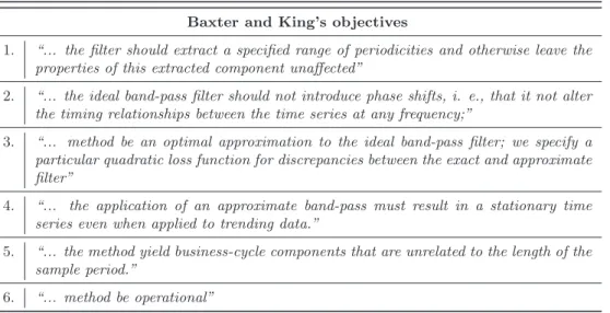
Baxter and King (1999) propose an approximate filter to extract business cycle fluctuations from a time series based on six criteria that restrain the filter design; see table 1.
Table 1: Baxter and King’s (1999) objectives to be met by their optimal approximation.
Baxter and King’s objectives
1. “... the filter should extract a specified range of periodicities and otherwise leave the properties of this extracted component unaffected”
2. “... the ideal band-pass filter should not introduce phase shifts, i. e., that it not alter the timing relationships between the time series at any frequency;”
3. “... method be an optimal approximation to the ideal band-pass filter; we specify a particular quadratic loss function for discrepancies between the exact and approximate filter”
4. “... the application of an approximate band-pass must result in a stationary time series even when applied to trending data.”
5. “... the method yield business-cycle components that are unrelated to the length of the sample period.”
6. “... method be operational”
The first entry in table 1 means that the ideal filter is a band-pass filter with a gain function of one over the [−ωu;−ωl]∪[ωl;ωu] frequency range and zero at all other frequencies, exactly as in equation (6).
To avoid phase shifts (second objective in table 1) it is necessary to set the phase of the filter equal to zero. The complex nature of the frequency response function,B¡e−iω¢, implies a polar representation as follows
B¡e−iω¢=¯¯B¡e−iω¢¯¯e−iθ(ω)
where¯¯B¡e−iω¢¯¯denotes the gain andθ(ω) the phase of the filter. Therefore, the second objective corresponds to settingθ(ω) = 0 in the previous equation, which implies:
The fourth objective is attained under two restrictions: first the optimal weights must be symmetric and second must sum to zero. Mathematically,
bkj=bk−j ∀j ⇒BK(L) =bko+ K
X
j=1
bkj
¡
Lj+L−j¢ (8)
BK(1) = K
X
j=−K
bkj=bko+ 2 K
X
j=1
bkj= 0 (9)
where BK(L) = PKj=−KbkjLj is the time domain representation of Baxter and King’s ap-proximate filter (BK filter) andK the maximum lag length5. In the frequency domain we are
constraining the response of the filter to be zero at the zero frequency, which is intuitive since low frequencies are related to the trend component. Nevertheless, these assumptions do not restrict the trend to be stochastic. In fact, Baxter and King (1999) prove that these two assumptions remove either stochastic trends up to second order or up to quadratic deterministic trends.
The last two objectives in table 1 state that the weights should not be time-dependent and that the method should be of easy implementation. Finally, the third objective describes how the weights of the approximate filter are obtained in order to have an optimal approximation to the ideal symmetric band-pass filter.
Adding the constraint in equation (9), to ensure a trend elimination property in the approx-imate filter, the weights of the BK filter solve the following optimization problem:
M in
{bkj}j=−K,...,K
E ∞ X
j=−∞
bjyt−j− K
X
j=−K bkjyt−j
2
s.t. BK(1) = K
X
j=−K
bkj =bko+ 2 K
X
j=1
bkj= 0
where©bj:j = 0,+−1, . . .
ª
denotes the weights of the ideal band-pass filter and©bkj :j= 0,+−1, ...,+−K
ª
the weights of the optimal filter. In the frequency domain we have
M in
{bkj}j=−K,...,K Z π
−π
¯
¯B¡e−iω¢−BK¡e−iω¢¯¯2dω
s.t. BK(1) = K
X
j=−K
bkj =bko+ 2 K
X
j=1
bkj= 0
where B(z) = P∞j=−∞bjzj and BK(z) = PKj=−Kbkjzj with z taken to be a complex scalar. The objective function written in frequency domain reveals that Baxter and King implicitly assume an independent and identically distributed (i.i.d.) process for the time seriesytsince no spectrum appears in the objective function. As a result, the square error terms are all equally weighted and the optimal weights will not directly depend on the true data generating process (DGP).
The 2K+ 1 weights of the approximate filter are obtained from the first order conditions (FOC) derived from the implied Lagrange function:
L(bk−K, . . . , bkK, λ) =
Z π
−π
¯
¯B¡e−iω¢−BK¡e−iω¢¯¯2dω−λ K
X
j=−K bkj
∂L(bk−K,...,bkK,λ)
∂bkj =−
Rπ
−π
¡
e−iωj+eiωj¢ £B¡e−iω¢−BK¡e−iω¢¤dω−λ= 0, j =−K, ..., K ∂L(bk−K,...,bkK,λ)
∂λ =−BK(1) = 0
After some algebraic manipulations6 we obtain
bkj =bj+4λπ =bj−
bo+2PKj=1bj
1+2K , j =−K, ..., K λ =− 4π
2K+1
³
bo+ 2PKj=1bj
´
where ©bj :j= 0,+−1, ...
ª
represent the weights of the ideal band-pass filter. The BK optimal weights have a few interesting features. First, they only depend on the weights of the ideal band-pass filter and on the nonnegative integer Kthat truncates the moving average. This indicates that the BK approximate filter also satisfies the sixth criterion, i.e., easy implementation. Second, the BK weights just differ from the ideal weights by a standardization factor λ
2.1.2 The Christiano and Fitzgerald approximation
Baxter and King’s approximation to the filter that ideally isolates business cycle fluctuations has two important flaws; first it is unsuitable for real-time analysis and second does not take into account the true DGP. The approximate filter proposed by Christiano and Fitzgerald (2003) surmounts both limitations by defining the solution as a function of all available data points and using the spectrum of the series to be filtered as a weighting function of the approximation errors. However, their approach is not a complete novelty in the literature. Geweke (1978) and Pierce (1980) have presented the time domain solution to the same problem analyzed in Christiano and Fitzgerald (2003) but in the context of seasonal adjustment. It is shown that the best approximation to the filter is equivalent to apply the ideal filter to the series of interest, but with the particularity that this series is extended with optimal backcasts and forecast when data points are not available. The solution proposed by Geweke (1978) allows for the inclusion of multivariate information but does not deal with unit root processes whereas Pierce (1980) deals with unit roots but only in a univariate context. So, Christiano and Fiztgerald’s (2003) contribution is the derivation of the solution to the problem of extracting business cycle fluctuations in real-time in a frequency domain perspective.
They start by assuming a time series decomposition as in equation (2) and set their approx-imate filter as the solution toT (sample length) projection problems defined as follows
ˆ
xt=P(xt/ℑT) , t= 1,2, ..., T
where ℑT denotes the available information set. The solution is a linear combination of the available data
ˆ xt=
p
X
j=−f
cftjyt−j =CFt(L)yt, t= 1,2, ..., T
For a given t the optimal weights solve the following optimization problem written in the fre-quency domain:
M in
{cfj}j=−f,...,p Z π
−π
¯
¯B¡e−iω¢−CF¡e−iω¢¯¯2Sy(ω)dω
where B(z) = P∞j=−∞bjzj is the frequency response function of the ideal filter, CF(z) =
Pp j=−fcf
p,f
j zj is the frequency response function of the optimal filter andSy(w) is the spectrum of yt. In contrast with the BK objective function, the errors between the ideal filter and the optimal filter are penalized by the spectrum of yt which implies that the loss function will explicitly depend on the choice of the time series representation. Furthermore, because the weights vary over time the optimization problem must be solved for each sample observation in order to get theT sets of weights needed to extract the desired component.
Christiano and Fitzgerald’s MSE filter is derived and analyzed in detail in the working paper version of Christiano and Fitzgerald (2003) for two types of processes. Following their notation let
yt=yt−1+θ(L)εt
whereεtis a zero mean white noise process withE(ε2t) = 1 andθ(L) =θ0+θ1L+θ2L2+...+θqLq, a finiteqorder lag polynomial. When θ(1) = 0,ytis a zero mean covariance stationary process modeled as
yt=yt−1+θ(L)εt⇔yt= θ(L)
1−Lεt⇔yt= ˜θ(L)εt
with ˜θ(L) a (q−1) lag polynomial. When θ(1) 6= 0, yt is a unit root process, i.e., difference stationary. Finally, ifθ(1)6= 0 andθ(L) = 1, ytis a random walk process
yt=yt−1+εt.
In general the spectral density function is
Sy(ω) = 1 2π
(
γy(0) + 2
+∞
X
k=1
γy(k) cos(ωk)
)
=
= 1 2π
θ(e−iω)θ(e−iω)
(1−e−iω) (1−eiω), −π≤ω≤π
where g(ω) = θ(e−iω)θ(eiω) = c
0+c1¡e−iω+eiω¢+...+cq
¡
e−iωq+eiωq¢. Thus c
∀τ and cτ = 0 for τ > q, reflecting that
h
c0 c1 ... cq
i
are constants that follow from the covariance function ofθ(L)εt.
In the non-stationary case we have to ensure that the filtered series is covariance stationary since no symmetry is forced upon the weights. Accordingly, the optimal filter weights must sum to zero
CF(1) = p
X
j=−f
cfj= 0
following that7
CF∗(L) = CF(L)
(1−L) whereCF∗(L) =Pp−1
j=−fcf
∗
jLj =cfp∗−1Lp−1+...+cf−∗fL−f. Through the method of indeter-minate coefficients we obtain a relationship between the weights of both filters
cfj∗=− p
X
k=j+1
cfk, j=p−1, ...,−f
or in matrix form
cf∗=Q·cf ⇔ cf∗
p−1
cf∗
p−2
.. . cf∗ −f
| {z }
(p+f)×1
=
−1 0 · · · 0 0
−1 −1 · · · 0 0
..
. ... . .. ... ...
−1 −1 · · · −1 0
| {z }
(p+f)×(p+f+1)
· cfp cfp−1
.. . cf−f
| {z }
(p+f+1)×1
7IfL= 1 is a root of the lag polynomialCF(L) then the latter can be factorize as
CF(L) = (1−L)CF∗
(L)⇔CF∗
(L) = CF(L) (1−L)
withCF∗
(L) =Pp−1
j=−fcf
∗
jLj=cf
∗
p−1Lp
−1+...+cf∗ −fL
Adding the constraint and replacingSy(w) in the objective function follows8
M in
{cfj}j=−f,...,p Z π
−π
¯ ¯
¯ eB¡e−iω¢−CF∗(e−iw)¯¯
¯
2
g(e−iω)dω
s.t. CF(1) = p
X
j=−f cfj= 0
where Be(z) = (1B−(zz)) with z taken to be a complex number. The FOC’s of this minimization problem are Rπ
−πBe
¡
e−iω¢g(e−iω)eiωjdω=Rπ
−πCF
∗(e−iω)g(e−iω)eiωjdω, j=p−1, ...,−f
CF(1) =cfp+...+cf−f= 0
Christiano and Fitzgerald solve this problem by replacing the first p+f conditions by a system of linear equations incfj,j=p, . . . ,−f such as
R(j)−R(j−1) =S(j)−S(j−1), j=p−1, . . . ,−f+ 1 (10)
R(−f) =S(−f) (11)
with R(j) = R−ππBe¡e−iwω¢g(e−iω)eiωjdω and S(j) = Rπ
−πCF
∗(e−iω)g(e−iω)eiωjdω for j = p−1, . . . ,−f. The left side of equation (10) equals
R(j)−R(j−1) =
Z π
−π
B¡e−iω¢g(e−iω)eiωjdω=
=
2πbjθ02 ,ifq= 0
2π¡bjc0+Pqi=1£b|j|+i+b|j|−i
¤
ci
¢
,ifq >0 8Note that,
Q =
Z π
−π
¯
¯B¡e−iω¢−CF¡e−iω¢¯¯2S
y(ω)dω=
=
Z π
−π
¯
¯B¡e−iω¢−CF¡e−iω¢¯¯2 g(e
−iω)
(1−e−iω) (1−eiω)dω=
= Z π −π ¯ ¯ ¯ ¯ ¯
B¡e−iω¢
(1−e−iω)−
CF¡e−iω¢
(1−e−iω)
¯ ¯ ¯ ¯ ¯ 2
g(e−iω)dω=
=
Z π
−π
¯ ¯
¯ eB¡e−iω¢−CF∗
(e−iω)¯¯
for j =p−1, . . . ,−f + 1 and where {bj} are the ideal weights as in equation (4). While, the right side of equation (10) equals
S(j)−S(j−1) =
Z π
−π
CF(e−iω)g(e−iω)eiωjdω=
=
2π·cfj·θ02 ,ifq= 0
2π·Aj·cf ,ifq >0
forj =p−1, . . . ,−f+ 1 and where {cfj} are the optimal weights, cf is a (p+f+ 1) column vector cf =hcfp · · · cf0 · · · cf−f
i′
and Aj is a (p+f + 1) row vector that involves the constants cτ, τ = 0, ..., q, and that varies according to the values of j9. Finally, equation (11) translates to
Z ωu
ωl ·
e−iωf 1−e−iω +
eiωf 1−eiω
¸
g(e−iω)dω= 2π·F·Q·cf= 2π·A−f·cf
where F is a (p+f) row vector F =h0 · · · 0 cq cq−1 · · · c0
i
while Qand cf mantain the same definitions as above.
At last, the (p+f+ 1) optimal weights for the non-stationary case are obtained by solving the following linear system
d= 2π·A·cf ⇔ Rπ
−πB
¡
e−iω¢g(e−iω)eiω(p−1)dω
.. .
Rπ
−πB
¡
e−iω¢g(e−iω)eiω(−f+1)dω
Rωu
ωl h
e−iωf 1−e−iω +
eiωf 1−eiω
i
g(e−iω)dω 0
| {z }
=
(p+f+1)×1
2π·
Ap−1
.. . A−f+1
A−f ι
| {z }
(p+f+1)×(p+f+1)
· cfp .. . cf−f+2
cf−f+1
cf−f
| {z }
(p+f+1)×1
For the stationary case we drop the constraint imposed over the zero frequency of the fre-quency response function. So, only small adjustments are done to adapt the linear system to the stationary case. In detail, the last two rows ofA are replaced byAp andA−f, respectively, and the last two rows ofdare replaced byR−ππB¡e−iω¢g(e−iω)eiωldω forl=pand−f.
for the non-stationary case settingq= 0 andθ0= 1. These assumptions imply
yt=yt−1+εt withE(ε2t) = 1 Sy(ω) =
1 2π
1
(1−e−iω) (1−eiω), −π≤ω≤π
and
M in
{cfj}j=−f,...,p Z π
−π
¯ ¯
¯ eB¡e−iω¢−CF∗(e−iω)¯¯¯
2
dω
s.t. CF(1) = p
X
j=−f cfj= 0
From this minimization problem we get a closed form expression for the optimal weights which simplifies the filtering procedure:
cfj=
1 2b0−
Pj−1
k=0bk , j =p
bj , j =p−1, ...,−f+ 1
1 2b0−
P0
k=j+1bk , j =−f
, t= 1, ..., T
where p=t−1,f =T −1 and {bj} stands for the weights of the ideal band-pass filter given in equation (4). It is worth noting that most optimal weights are equal to the ideal weights and that only the highest order terms are adjusted to ensure the stationarity of the filtered series. This particular filter is known in the literature as the optimal random walk filter. The random walk filter is a symmetric filter whenp=f. First note that cfj =bj forj =p−1, ...,1−pand that the ideal weights are symmetric. Secondly, it is easily proven that cfp =cf−p replacing j bypand−pin the expressions above. Forp=f andpfixed we have
cfjp,p=bj− 1 1 + 2p
b0+ 2
p
X
j=1
bj
, j= 0,+−1, ...,+−p
constraints (assumingp=f andpfix) and so the optimal weights are just a truncated version of the ideal weights. A near i.i.d. case corresponds to the BK case when we impose the stationarity condition of the filtered series. In this case the optimal weights are the ideal weights truncated and adjusted by a constant in order to verifyBK(1) = 0 andbkj =bk−j ∀j.
Although the CF filter is made optimal according to the DGP, Christiano and Fitzgerald concluded that the pure random walk filter is nearly optimal even if the random walk process is not the true time series representation. A reason that can justified this result is the fact that many of the U.S. time series exhibit what is called a typical Granger spectral shape, in other words most series exhibit a low dominating spectrum. Nevertheless, gains are always achieved by using the true time series model in the optimization problem but they can be rather small when compared with the effort needed to run a model choice procedure or to implement the optimal procedure with the true DGP. Finally, they also stress that important efficiency gains are attained using all information available at each timet.
2.1.3 The Multivariate approximation
For the same frequency extraction problem of Christiano and Fitzgerald (2003), Valle e Azevedo (2007) has developed a multivariate approximation. Basically, he expands the CF univariate so-lution adding an arbitrary number of covariates to the soso-lution. The idea is that those additional covariates will help to improve the estimate of the desired frequency component, in particular at the endpoints where the estimates are frequently poor.
expressed as
ˆ xt=
p
X
j=−f ˆ Bjyt−j+
n
X
s=1
p
X
j=−f ˆ
Rs,jzs,t−j= ˆB(L)yt+ n
X
s=1
ˆ
Rs(L)zst (12)
wherepdenotes the number of past observations,f the number of future observations used from
the available information set at each time t and
n
ˆ
Bj; ˆRs,j:j =−f, . . . , p;s= 1, . . . , n
o
are the (n+ 1)×(p+f + 1) weights of the optimal multivariate filter. Such weights are chosen in such a way that the minimum MSE estimate of the ideally filtered series at timet is obtained, i.e.,
M in
{Bˆj; ˆR1,j;...; ˆRn,j} j=−f,...,p
E[(xt−xbt)2].
The frequency domain formulation of the problem is now slightly different since it involves a vector process10
M in
{Bˆj; ˆR1,j;...; ˆRn,j} j=−f,...,p
Z π
−π
β(ω)Sy,z1,...,zn(ω)β
′∗(ω)
where β(ω) = hB¡e−iω¢−Bˆ¡e−iω¢ −Rˆ
1
¡
e−iω¢ · · · −Rˆ n
¡
e−iω¢i, B(z) =P∞j=−∞Bjzj, ˆB(z) =Ppj=−fBˆjzj, ˆRs(z) =Ppj=−fRˆjzj fors= 1, . . . , nandSy,z1,...,zn(w)
denotes the (n+ 1)×(n+ 1) spectral matrix of the vector processhy z1 · · · zn
i′
.
The solution to this multivariate optimization problem is derived in Valle e Azevedo (2007) assuming a M finite order moving average (MA(M)) representation for the vector process, as in
10ConsideringWta covariance stationary vector then its spectrum is
SW(ω) =
1 2π
∞ X
k=−∞
Γ(k)e−iωk, −π≤ω≤π
whereΓ(k) denotes the covariance matrix, which can be recovered from the spectrum by
Γ(k) =
Z π
−π
SW(ω)eiωkdω, k= 0,+−1,
+
−2, ...
Hence, the spectrum of the filtered seriesMt=P∞j=−∞HjWt−jis
SM(ω) =H(e
−iω)S
W(ω)H
′
(eiω), −π≤ω≤π
Note that it generalizes the univariate case. Suppose thatWtis a univariate covariance stationary process then
SM(ω) =H(e
−iω)S W(ω)H
′
(eiω) = =H(e−iω)H(eiω)S
W(ω) =
=¯¯H(e−iω
Christiano and Fitzgerald (2003). Nonetheless, the case of non-stationarity of the series to be filtered is also handled. If yt is a unit-root process then to ensure stationarity of the filtered series the previous problem is constrained with
ˆ
B(1) = 0⇒Bˆ(z) = (1−z)b(z)⇔b(z) = ˆB(z)/(1−z)
whereb(z) =Ppj=−−1fbjLj=bp−1zp−1+...+b0+b−fz−f and so the objective function is modified to
M in
{Bˆj; ˆR1,j;...; ˆRn,j}j=−f,...,p Z π
−π
α(ω)S∆y,z1,...,zn(ω)α(−ω)
′
with α(ω) = hB¯¡e−iω¢−b¡e−iω¢ −Rˆ
1¡e−iω¢ · · · −Rˆn
¡
e−iω¢i, ¯
B(z) = B(z)/(1 − z) and S∆y,z1,...,zn(ω) is the spectrum of the vector process h
∆y z1 · · · zn
i′
.
Define Wj as a (n+ 1) column vector
h
bj Rˆ1,j · · · Rˆn,j
i′
, j = p−1, ...,−f, then the FOC’s are ∂L
∂Wj = 0⇔ Rπ
−πe
−iωj
S∆y(ω) Sz1,∆y(ω)
.. . Szn,∆y(ω)
¯
B¡e−iω¢dω=Rπ
−πe
−iωjS
∆y,z1,...,zn(ω)
b¡eiω¢ ˆ R1
¡
eiω¢ .. . ˆ Rn
¡
eiω¢
dw ∂L
∂λ = 0⇔Bˆ(1) = 0
forj=p−1, . . . ,−f.
Following the strategy of Christiano and Fitzgerald the (n+ 1)×(p+f) first equations of the FOC’s are replaced by other equations. Define the left hand side as
Sj =
Z π
−π e−iωjS¯
∆y,z1,...,zn(ω) ¯B ¡
then
Sj−Sj−1=
Bjγ∆y(0) +PMi=1(Bj+i+Bj−i)γ∆y(i) ..
. Bjγzn,∆y(0) +
PM
i=1(Bj−iγzn,∆y(i) +Bj+iγzn,∆y(i)) =Vj
forj=p−1, ...,−f + 1. TheSj are then obtained recursively by
Sj =Sj−1+Vj, j=p−1, ...,−f+ 1.
For−f we evaluate the following integral numerically
S−f =
Z −ωl
−ωu
eiωf
1−eiωS¯∆y,z1,...,zn(ω)dω+ Z ωu
ωl
eiωf
1−eiωS¯∆y,z1,...,zn(ω)dω.
The right hand side of the FOC’s is replaced by
Rj=
Z π
−π e−iωjS
∆y,z1,...,zn(ω)
b¡eiω¢ ˆ R1¡eiω¢
.. . ˆ Rn¡eiω¢
dω=QjW ,ˆ j=p−1, ...,−f
withQj=
Q∆y,j Q∆yz1,j · · · Q∆yzn,j
..
. ... . .. ... Qzn∆y,j Qznz1,j · · · Qzn,j
11and ˆW =hˆ
B R1 · · · Rn
i′
a column vector
with all weights stacked.
Finally, only n+ 1 conditions that correspond to the case j =pare missing. The weights
n
ˆ
R1,p;...; ˆRn,p
o
are obtained from ˜Sp= ˜QpWˆ, where ˜Sp equalsSp but with the first row deleted and ˜QpequalsQpwith the first row deleted. The final equation is given by the restriction impose at the beginning, ˆB(1) = 0, which gives ˆBp.
So, the optimal weights ˆW solve a linear system with (n+ 1)×(p+f+ 1) equations
V =QWˆ ⇔Wˆ =Q−1V (13)
11For further details on the definition of theQ
with V = hS−f · · · Sp−1 S˜p 0
i′
[(n+1)×(p+f+1)]×1,
Q=hQ−f · · · Qp−1 Q˜p U
i′
[(n+1)×(p+f+1)]×[(n+1)×(p+f+1)],
ˆ
W =hBˆ R1 · · · Rni′
[(n+1)×(p+f+1)]×1 andU =
h
1 · · · 1 0 · · · 0
i
.
To accommodate the case in which all data points are used, one just setsp=t−1 andf =T−t and solves the linear system in equation (13)T times, like in Christiano and Fitzgerald. In the stationary case no restriction is imposed and some adjustments are done to theV andQmatrices
V =QWˆ ⇔Wˆ =Q−1V
with V = hS−f · · · Sp−1 Sp
i′
, Q = hQ−f · · · Qp−1 Qp
i′
and the spectrum is from Sy,z1,...,zn(w) because now it is implied that yt is a covariance stationary process. The optimal
weights, i.e., the solution of the optimization problem depends (a) on the second order moments ofh∆y, z1, . . . , zn
i
orhy, z1, ..., zn
i
, due to the presence of the spectrum in the objective function and (b) on the ideal weights as given in equation (4). Moreover, this filter does not remove stochastic or deterministic trends due to the asymmetrical weights.
As pointed out in the context of Christiano and Fitzgerard’s filter, this type of solution cannot be seen as completely new in the literature given the studies of Geweke (1978) and Pierce (1980). But this particular approach has an important contribution since it gives the extension to the multivariate case of the solution obtained when filtering a unit root process.
2.1.4 The Hodrick and Prescott filter
In order to analyze the cyclical component of some macroeconomic variables, Hodrick and Prescott (1980, 1997) developed a detrending method based on the idea that a time series is the sum of two unobservable and uncorrelated components:
yt=gt+ct, t= 1, ..., T (14)
cost function
M in
{gt}t=1,...,T
T
X
t=1
(yt−gt)2+λ TX−1
t=2
[(gt+1−gt)−(gt−gt−1)]2. (15)
Since the average of the deviations from the trend is expected to be near zero for long time periods, the first term of the objective function sums the squares of those deviations. The second term sums the variation in the second difference of the growth component, £(1−L)2g
t
¤
where Ldenotes the lag operator, which gives the variability of the growth component (trend growth rate). Hodrick and Prescott state that this measures the smoothness of the long run component, expected to evolve smoothly over time, and thus penalize this term by a positive number λ, known as the smoothness parameter. The larger λ is the smoother is the growth component. If λ= 0 then the first term of the objective function in equation (15) has to be zero in order to minimize the function. As a result, the growth component equals the original series and the cyclical movements do not exist. In the limit, when λ = ∞, we have perfect smoothing, the growth component is simply a linear trend, and we obtain the maximum cyclical fluctuations. The smoothing parameter is not determined by optimization but derived in Hodrick and Prescott (1980, 1997) from a probability model. They show that if the cycle component and the second difference of the trend are zero mean i.i.d. normally distributed variables then the parameter equals the variance of the business cycle component divided by the variance of the acceleration in the trend component,λ12 =σc/σ∆2g. From this formula results the standard valueλ= 1600 for
quarterly data. For other data frequencies some correction has to be done due to alterations in the variability of the series. Adjustment rules have been suggested by Backus and Kehoe (1992), Correia et al. (1992), Cooley and Ohanian (1991) and Ravn and Uhlig (2001). Alternatively, in the working paper version of Canova (1998) the smoothing parameter is understood as a signal extraction coefficient and is estimated by maximum likelihood. Also, Harvey and Jaeger (1993) attempt to estimate the parameter using maximum likelihood methods.
The FOC’s from equation (15) are
−2 (yt−gt) + 2λ[(gt−gt−1)−(gt−1−gt−2)]−4λ[(gt+1−gt)−(gt−gt−1)]
+ 2λ[(gt+2−gt+1)−(gt+1−gt)] = 0, t= 1, . . . , T (16)
using the backshift and forwardshift operator,Lj andL−j, respectively, i.e.,
yt =
£
λ(1−L)2(1−L−1)2+ 1¤gt⇔
⇔ gt=
1
1 +λ(1−L)2(1−L−1)2yt⇔
⇔ gt=G(L)yt, t= 1, . . . , T
Thus, the growth component is obtained from the original series by applying a linear filter to the raw data. The filterG(L) is known as the HP growth filter and essentially consists in a low pass filter since it aims to extract only the long run movements associated to low frequencies. Straightforwardly, the HP cyclical filter is obtained as,
ct=yt−gt= [1−G(L)]yt=C(L)yt
whereC(L) =£λ(1−L)2(1−L−1)2¤/£1 +λ(1−L)2(1−L−1)2¤. TheC(L) filter is a high pass
filter that renders stationary any integrated process up to fourth order and that induces no phase shift due to symmetry.
Unlike the discussed optimal filters, the growth or cyclical HP filter is not presented, in the original framework, as an optimal solution to a frequency extraction problem. But, King and Rebelo (1993), section 4, show that for an infinite sample and a particular class of models the HP cyclical filter is the optimal approximation, in the MSE sense, to an ideal high pass filter. Due to this interpretation and the broadly use of the HP method for detrending time series, it is common practice to use this filtering technique as a benchmark when evaluating the performance of alternative procedures (see Baxter and King, 1999, Christiano and Fitzgerald, 2003 or Valle e Azevedo, 2007).
Assuming that the weights are square summable there is a valid Fourier transform of the cyclical HP filter. King and Rebelo (1993) showed that the transfer function12 is given by
C(w) = 4λ[1−cos(w)]
2
1 + 4λ[1−cos(w)]2, −π≤w≤π.
Hence, the frequency domain approach stresses the trend elimination properties of the filter because zero weight is placed on the zero frequency, C(0) = 0, and the fact that it does not
reweight the high frequencies since almost unit weight is placed on those frequencies.
This tool gained popularity given its use in the context of Real Business Cycle (RBC) models. In this context, the HP filter is used in a preliminary step to eliminate the trend component of several variables. The choice of the HP filter as a detrending method follows from its flexibility to incorporate (through the smoothness parameter) the researchers’ preferences regarding the path of the trend.
2.2
Comparison
In this subsection we examine the limitations of the discussed approximate filters and simultane-ously document their differences and similarities. This exercise is important to establish which filters may be used to construct a real time indicator (our main objective). We will focus our analysis on the filters that aim to approximate business cycle fluctuations, simply because these were the kind of filters that we discussed in more detail in the previous subsections. However, most of the conclusions are also valid for smooth growth approximate filters.
The HP and BK approximations are optimal in MSE sense under a particular set of conditions, hardly met in our particular application to GDP series. In the case of the HP filter such conditions imply assuming that the trend of a time series is integrated of order two and that the cyclical fluctuations follow a white noise process. In the case of the BK filter the implicit assumption considers that the time series to be filtered follows an i.i.d. process.
concentrated around the lowest frequency and no spurious cycles are in fact induced by applying these filters to integrated time series. Intuitively, if the spectrum of a time series is dominated by low frequencies then it is hard to identify the business cycle fluctuations in the original series. Automatically the peaks in the spectrum of the filtered series are interpreted as distorted cycles when in fact they represent fluctuations that are definitely present in the time series.
Secondly, the HP filter is mainly a detrending method and less orientated to the measurement of business cycle fluctuations given the adopted definition. The so-called cyclical component of Hodrick and Prescott is obtained from the difference between the observed time series and the estimated growth component. Thus, unlike all the other business cycle approximation filters, discussed in the previous subsections, the noise component connected to very high frequencies is not removed but absorbed by the cyclical component. This might explain why in figure 2 panel A the HP approximation to business cycle fluctuations of real GDP is more ragged than the alternative approximations.
Figure 2: Approximations to the business cycle fluctuations of U.S. real GDP using alternative filtering techniques.
1963 1967 1971 1875 1979 1983 1987 1991 1995 1999 −5
−4 −3 −2 −1 0 1 2 3 4
percent
panel A
HP λ = 1600 BK K=12
1963 1967 1971 1875 1979 1983 1987 1991 1995 1999 −5
−4 −3 −2 −1 0 1 2 3 4 5
percent
panel B
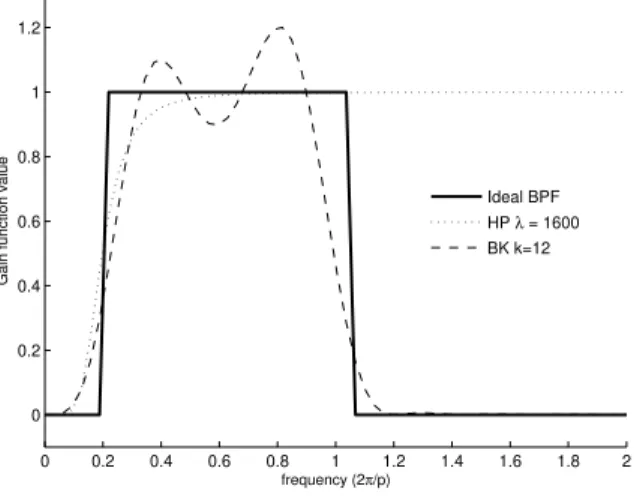
In fact the extracted components are not directly comparable because we are extracting different types of information from the data. This reveals that the definition of business cycle fluctuations is arbitrary and can be model-dependent. Moreover, if the HP cyclical filter retains both medium and high frequencies from a time series then it is expected to better approximate an ideal high pass filter than an ideal band-pass filter. Figures 3 (panel B) and 4 show that it is in fact the case. For the standard value ofλ= 1600 the HP cyclical filter contains minor problems of leakage and compression and so is considered as a good approximation to the high pass filter with cutoff frequencyω = 2π
32. Instead, the trend filter will retain only the long periodicities, suggesting a
good approximation to an ideal low pass filter as revealed by figure 3 panel A.
Figure 3: Panel A. Gain function of the ideal low pass filter that retains cycles of length lower than 32 quarters against the gain function of the Hodrick and Prescott growth filter withλ= 1600; Panel B. Gain function of the ideal high pass filter that retains cycles of length higher than 32 quarters against the gain function of the Hodrick and Prescott cyclical filter withλ= 1600.
−1 −0.8 −0.6 −0.4 −0.2 0 0.2 0.4 0.6 0.8 1 0
0.1 0.2 0.3 0.4 0.5 0.6 0.7 0.8 0.9 1
frequency (2π/p)
Gain function value
panel A
Ideal LPF
λHP = 400
λHP = 1600
λHP = 6400
−1 −0.8 −0.6 −0.4 −0.2 0 0.2 0.4 0.6 0.8 1 0
0.1 0.2 0.3 0.4 0.5 0.6 0.7 0.8 0.9 1
frequency (2π/p)
Gain function value
panel B
Ideal HPF
λHP = 400
λHP = 1600
Figure 4: Gain function of the ideal band-pass filter passing frequencies in the range 2π
32 ≤ |ω| ≤ 2π
6
against the gain function of the Hodrick and Prescott cyclical filter withλ= 1600 and the Baxter and King filter truncated at lag and lead 12.
0 0.2 0.4 0.6 0.8 1 1.2 1.4 1.6 1.8 2 0
0.2 0.4 0.6 0.8 1 1.2
frequency (2π/p)
Gain function value
Ideal BPF HP λ = 1600 BK k=12
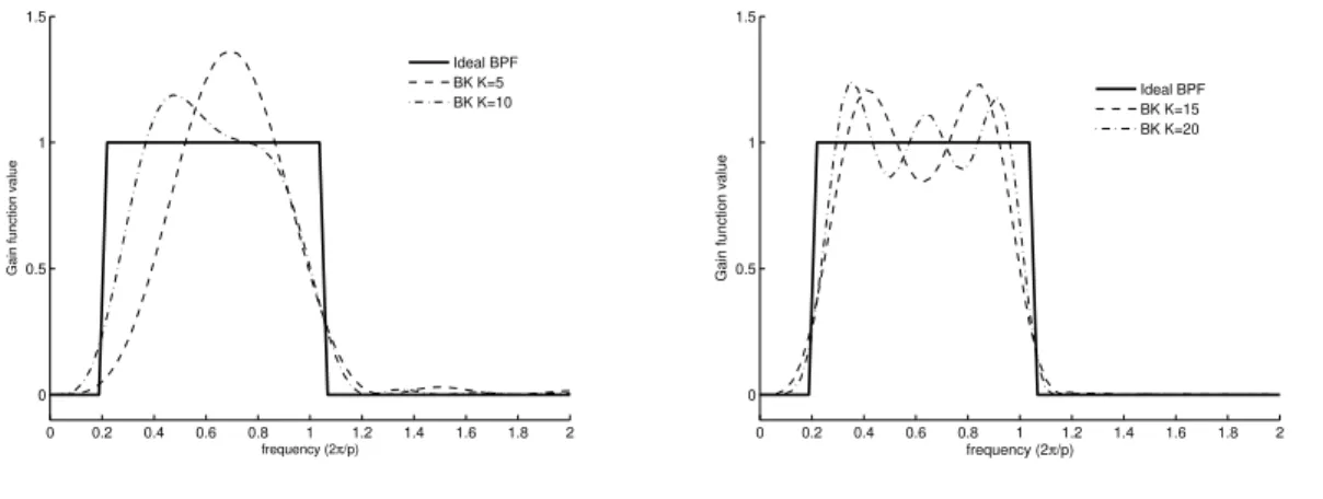
Figure 5: Gain function of the ideal band-pass filter passing frequencies in the range 2π
32 ≤ |ω| ≤ 2π
6 against
the gain function of the Baxter and King filter forK= 5,10,15,20.
0 0.2 0.4 0.6 0.8 1 1.2 1.4 1.6 1.8 2 0
0.5 1 1.5
frequency (2π/p)
Gain function value
Ideal BPF BK K=5 BK K=10
0 0.2 0.4 0.6 0.8 1 1.2 1.4 1.6 1.8 2 0
0.5 1 1.5
frequency (2π/p)
Gain function value
Ideal BPF BK K=15 BK K=20
For a final comparison between the HP and BK filters’ gains we analyse figure 4 that displays the gain function of the ideal band-pass filter withωl = 232π and ωh = 26π as cutoff frequencies
Figure 6: Approximation to the business cycle fluctuations of U.S. real GDP using the Baxter and King approximate filter with lag lengths of 5, 10, 15 and 20 quarters.
1960 1965 1970 1975 1980 1985 1990 1995 2000 −5
−4 −3 −2 −1 0 1 2 3 4
percent
K=5 K=10 K=15 K=20
Thirdly, several studies document that the smoothing parameter present in the HP filter should fit the data in terms of frequency and intrinsic properties, but theory provides little guidance as to what this value should be. Thus, in applied work the degree of smoothness is simply a matter of choice subject therefore to individual judgements. An inadequate choice of λ may lead to attribute variability to the cyclical component that in fact is part of the trend component. A similar caveat arises in the context of the BK optimal filter given the requirement of a prior choice of theKvalue (and also of the frequency band of interest). Evidently that increasing K enhances the approximation to the ideal filter but also implies loosing more observations at both endpoints of the sample. As before, there is no good rule for setting K but the advice is obvious: weight the trade off from the opposing factors when setting the truncation point of the infinite order MA filter. From simulation results, Baxter and King (1999) suggest, as guideline, that researchers use moving averages based on three years of past data and three years of future data, as well as the current observation, for quarterly and annual U.S. data.
overcome this particular limitation. Van Norden (2004) suggested without much success to use BK filter for the full sample length replacing by zero the missing observations. While Stock and Watson (1998) suggested to expand the sample with K forecasts and K backcasts generated from a suitable time series model. Moreover, this feature of the BK approximations may suggest that the HP approximations might be preferred over the first because the HP filter generates estimates for both components at the beginning and end of the sample. The finite version of the HP filter in time domain representation, derived in Hodrick and Prescott (1997), shows that the cyclical component at each momentt can be obtained through a linear filter with time-varying weights involving all available data points. The problem, is that the first and last filtered observations have very poor properties given the one-sided nature of the applied filter, as documented in Baxter and King (1999) and others. But this difficulty is shared with all methods that aim at obtaining estimates at the endpoints. In the analysis of HP filtered series typically some observations are disregarded but in that case we stay in the same situation of Baxter and King, no available real-time estimates.
Alternatives to the approaches discussed so far are the CF filter and the multivariate filter. Unlike HP and BK filters, these filters are made optimal according to the DGP. This implies different spectra in the objective function for each particular case. Nevertheless, the BK opti-mization problem is a special case of the CF optiopti-mization problem, and in turn the last is a special case of the multivariate filter. To obtain the CF filter from the multivariate problem the second term in the right side of equation (12) is dropped. So, the main difference between the two filters is that the multivariate method exploits additional information from a wide set of variables in order to get a more accurate estimate of the desired component, in particular at the endpoints. Theoretically, as Valle e Azevedo (2007) states better estimates will be obtained by applying the multivariate filter if the true second order moments were known. Since they have to be replaced by estimates it is not clear what happens.