Optimal design of active EMC filters

www.adv-radio-sci.net/11/243/2013/ doi:10.5194/ars-11-243-2013

© Author(s) 2013. CC Attribution 3.0 License.

Radio Science

Optimal design of active EMC filters

B. Chand, T. Kut, and S. Dickmann

Fundamentals of Electrical Engineering, Helmut Schmidt University / University of the Federal Armed Forces Hamburg, Germany

Correspondence to:B. Chand (benian.chand@hsu-hh.de)

Abstract. A recent trend in automotive industry is adding electrical drive systems to conventional drives. The electri-fication allows an expansion of energy sources and provides great opportunities for environmental friendly mobility. The electrical powertrain and its components can also cause dis-turbances which couple into nearby electronic control units and communication cables. Therefore the communication can be degraded or even permanently disrupted. To mini-mize these interferences, different approaches are possible. One possibility is to use EMC filters. However, the diversity of filters is very large and the determination of an appropriate filter for each application is time-consuming. Therefore, the filter design is determined by using a simulation tool includ-ing an effective optimization algorithm. This method leads to improvements in terms of weight, volume and cost.

1 Introduction

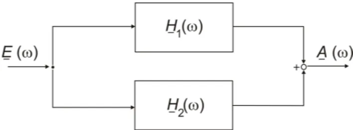
The EMC of electronic systems is often achieved by fil-ter networks. The used components take an increasing part of the total system weight and volume. Therefore, the op-timal filter for different requirements is determined with previous simulation estimations. The filters are character-ized in terms of the number and type of filter stages, com-ponent values or attenuation. Therefore passive, active and hybrid filter structures are used. The active filters are in-vestigated by using a feedforward structure (Fig. 1). Fur-thermore, the frequency characteristic of the filter is de-scribed by the use ofA

¯-matrices. The existing common- and differential-mode interferences are attenuated by an intercon-nection of common- and differential-mode filters. The input and output impedances are important design criteria. Taking into account these criteria, the manual design is very time-consuming due to the large number of possible filter struc-tures. Therefore, a algorithm was implemented which deter-mines the optimal filter network depending on the required

parameters. To determine the optimal filter for given bound-ary conditions the Particle Swarm Optimization (PSO) pro-cess is used. The output of the software includes not only the filter network topology and the component values, but also a comparison of the cost, weight and the simulation time. These results are verified by measurements. Finally, the de-termined filter is studied in a real, practical construction of an electrical powertrain.

2 Concepts of reducing the interferences by using EMC filters

We consider filter circuits which attenuate conducted inter-ference. Three groups of filter circuits are explained in this chapter: Passive, active and hybrid filters for common-mode and differential-mode. Parasitic effects are not taken into ac-count. Another topic of this section is the description of a two-port network by an A

¯-matrix. With these methods it is possible to determine the frequency characteristics of an electric filter circuit in a short time.

Passive filters

are the simplest form of electric filters (Hagmann, 2008). Since the components require no power supply, the combi-nation of these components are called passive filters. In this case, the filter should attenuate harmonics. For this reason, a low-pass topology will be used.

Active filters

Fig. 1.Positive feedback structure for active filtering.

Fig. 2.Schematic description of a four-terminal network.

the interferenceE

¯(ω)is conducted in parallel over the func-tionsH

¯1(ω)andH¯2(ω), so the unwanted interference can be canceled and the required output signalA

¯(ω)is produced.

Hybrid filters

circuits consist of active and passive filter circuits. The ad-vantage with such a configuration is the attenuation of the interference to a large amount by means of an active filter. Therefore, the passive components can be designed smaller, which can add to weight and cost savings.

Description of the filter using A

¯-Matrices

To determine the frequency characteristic of a filter circuit, A

¯-matrices can be used. In Fig. 2 a four-terminal network with its connections, the output and input current and the out-put and inout-put voltage is shown.

The system can be represented using a matrix notation:

U ¯e I ¯e =A ¯ · U ¯a I ¯a withA ¯ = A ¯11 A¯12 A

¯21 A¯22

(1)

The individual elements of the matrixA ¯ are:

A ¯11=

∂U ¯e ∂U ¯a _I

¯a=0 A

¯12= ∂U ¯e ∂I ¯a _U

¯a=0 A

¯21= ∂I ¯e ∂U ¯a _I

¯a=0 A

¯22= ∂I ¯e ∂I ¯a _U

¯a=0

(2)

Fig. 3.Series connection ofA

¯-matrices.

The advantage for a series connection ofA

¯-matrices, as described in Fig. 3, is the possibility to multiply the individ-ual matrices easily. The product results in an overall matrix. For the given overall matrix A

¯total, it is now possible to deter-mine the ratio of the input to output voltage. It follows from the inverse of the matrix elementA

¯11(Marti, 2007).

U ¯e I ¯e =A

¯1·A¯2·A¯3·. . .·A¯n−1·A_¯n·

U ¯a I ¯a (3) U ¯e I ¯e =_A

¯tot·

U ¯a I ¯a (4) For later considerations of active and hybrid filters theA

¯ -matrix of the active filter results from Fig. 5 (Rehfeld, 2012):

A ¯ =





s2·k1·L1·C1+s·C1·RC+1

s2_k

¯2·L1·C1+s·C1·RC+1

s·L1·(s·C1·RC1)

s2·L1·C1(κ ¯·(1+v)+

v

¨

u)+s·C1·RC+1

s·C1(1−κ ¯(1+v))

s2·k

¯2·L1·C1+s·C1·RC+1

1





with k1=1+vu¨, k_¯2=κ

¯·(v+1)+

v

¨

u, κ_¯=

U ¯OP U

¯e

, v=R2

R1,

¨

u=

q

L1

L2,s=j·2·π·f

Common-mode and differential-mode filters

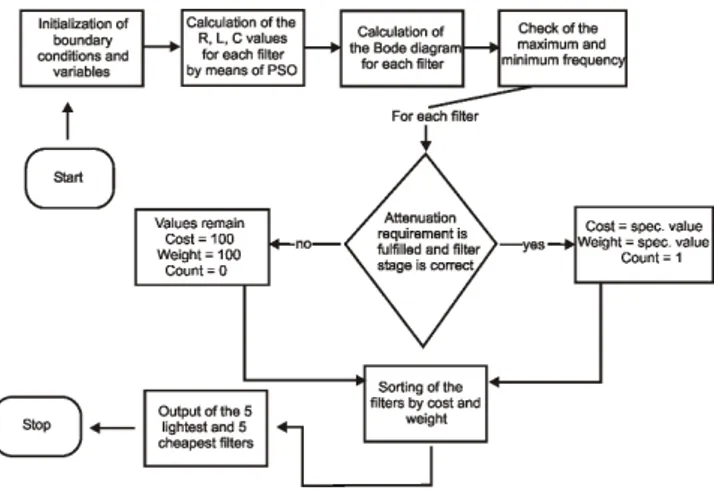
Fig. 4.Program Flowchart.

one wire and the ground and the same common-mode filter is used for the second wire as well. So the approach of 2×2 A

¯-matrices can be used here.

3 Design algorithm for EMC filters

3.1 Program flow of the simulation script

A program for designing electrical filters has been created. After entering the required attenuation in a certain frequency band, the script displays the cheapest and lightest filter topol-ogy for given boundary conditions. In this section, the algo-rithm of the script will be introduced and some important details are discussed.

With the help of a graphical user interface (GUI) the boundary conditions for the configuration of the filter circuit are set. These are the minimum and maximum values of the used inductors, capacitors and resistors (Lmin,Lmax, Cmin,

Cmax,Rmin,Rmax). Another input parameter is the

attenua-tion within a given frequency band. Furthermore, it should be determined, whether there is a high ohmic or a low ohmic input and output impedance, because they influence the be-havior of the filter circuit. Moreover, it is necessary to de-termine the number of the filter stages. For the evaluation, the program needs an input signal described in a text file. As output parameter of the script the required computing time or the calculated attenuation can be selected. In Fig. 4, the program flowchart of the main program is shown.

First of all, the entered boundary conditions are stored and initialized. In the next step, the various components of the different filter circuits are calculated. This is done using an optimization algorithm which is called Particle Swarm Opti-mization (PSO) (Brodersen, 2006). This process will be dis-cussed later in this section. After calculating the components of each filter, the frequency characteristic of the different fil-ter stages can be calculated throughout these components. For this purpose theA

¯-matrices of the filter circuits are used.

After comparing the input signal with the selected minimum and maximum frequencies, the program controls whether the filters are generally useable. On the one hand it is important, that the filter fulfills the required attenuation in the given fre-quency band and on the other hand it is checked whether the filter matches with the given filter stage. If these two condi-tions are met, the respective control variable “Count” is set to the value 1 and a specific value for the weight and price for this filter is defined. If the first condition is not fulfilled, the control variable “Count” is set to 0, the specific cost and the specific weight of the filter are set to the value 100. In the next step, the cost and weight of the filter are sorted by size, starting with the lowest. After that, the five filters with the lowest weight and the five filters with the smallest price will be displayed. Filters with the control variable “Count” = 0 are not considered.

3.2 Studied filter circuits

For the program and the later practical applications, it is necessary to consider different filter circuits. In the simula-tion program the following passive filter circuits are imple-mented to the fifth order: LC-, RC-, LRC-, T- andπ-filter. In active filters, operational amplifiers are used. The advan-tage of using operational amplifiers is the low weight and the low construction volume. The ideal operational amplifier, which is used in these simulations has the following charac-teristics: The internal impedance of the operational amplifier is infinitely large. The input currentI

¯e is zero. The output impedance of the operational amplifier is zero. The voltage gainAu,dfor differential signals is infinitely large. Therefore

the voltage between the input terminals is zero, when the out-put signal is limited. The common-mode rejection is infinite large.

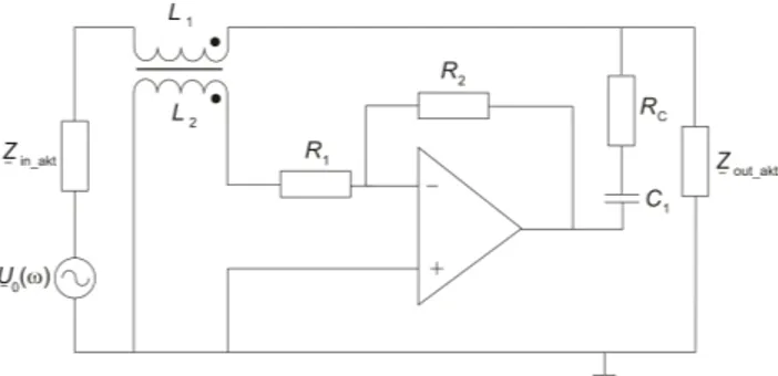
Previous studies (Rehfeld, 2012) have shown, that an ac-tive filter with an inducac-tive coupling and capaciac-tive decou-pling has the best filter characteristics. In these previous stud-ies different active filters with operational amplifiers were studied and the the active LC-filter in Fig. 5 was chosen. This filter is used for further considerations. It consists of a transformer, which decouples the interference signal via the inductanceL1and transmits it to the inductance L2, in the

secondary circuit. There, the decoupled signal is inverted by an inverter circuit and is transfered by means of the capacitor C1back to the load circuit.

3.3 Filter Optimization algorithm

Fig. 5.Active Filter with inductive coupling and capacitance decou-pling.

Fig. 6. Restriction condition for the PSO-algorithm (Brodersen, 2007).

3.3.1 Brute-Force-Method

The Brute-Force-Method tries each or a majority of all pos-sible solutions meeting the boundary conditions, until a so-lution is found. The advantage of this method is the deter-mination of an unique solution of the problem. However, the disadvantage is the requirement of high computing time due to an increasing number of variables in the solution space. 3.3.2 Ant-Colony-Algorithm

Another way to solve a complex problem is the Ant-Colony-Algorithm. Here, the natural behavior of ants when foraging is imitated. Each ant has a memory and also the entire ant colony has a collective memory. The ants have several possi-ble routes to reach the feeding place. The result of the algo-rithm is the optimal way to the food source (Boysen, 2006). This method is used very often for the optimization of busi-ness processes. It would also be possible to design filters with this process.

3.3.3 Particle-Swarm-Optimization

Another solution method is the Particle-Swarm-Optimization (PSO). This process provided good results in the field of en-gineering, e.g. in the construction of bandpass filters or the design of gears and can be applied to the current problem. The algorithm will be described more in detail below and is adapted to the problem of filter design.

Mathematical description:

Basically, thei-th particle of a swarm is described by: – xi: current position of the particle

– vi: current velocity of the particle

– yi: best position of the particle

In addition, a certain fitness functionf (xi)is assumed.

From this function we obtain the so called fitness value, that indicates how far the current position is away from the target. From the fitness value the next best position results:

yi(t+1)=

yi(t ) iff (xi(t+1)) < f (yi(t ))

xi(t+1)iff (xi(t+1))≥f (yi(t )) (5)

The next important parameter of the PSO is the swarm. It consists ofpparticles. The swarm has a collective mem-ory, which remembers the best position of the particle with the highest fitness value. This value is called the global best position. It is given by:

ygb(t+1)=

=

ygb(t ) iff y0...p(t+1)< f ygb(t )

y0...p(t+1)_maxiff y0...p(t+1)≥f ygb(t )

From the best position of each particle and the global best position, the new velocity of a particle is results:

vi(t+1)=w·vi(t )+c1r1(t )·

[yi(t )−xi(t )]+c2r2(t )ygb(t )−xi(t ) (6)

With the variables:

0≤c1, c2, w≤2 (7)

The two functions r1(t )and r2(t )are random numbers

(Brodersen, 2006). After determining the new velocity of each particle, the new current position of the particle results:

xi(t+1)=xi(t )+vi(t+1)·1t (8)

This algorithm is repeated until (Wu, 2006): a. a particle has found the optimal position

b. it is certain, that the optimal position for the solution space does not exist

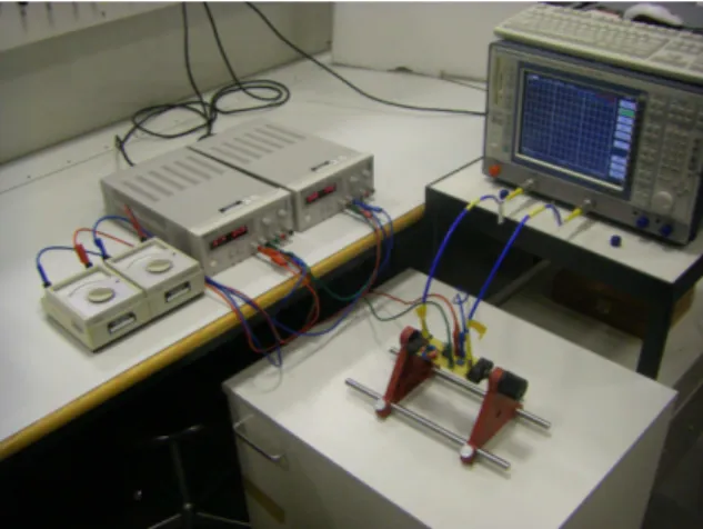
Fig. 7.Measurement setup for measuring the filter response.

shown. For the solution space the numbers from 0 to 10 are set. The white particle leaves the solution space. As a result, the black particle is created in the solution space, according to the following rules.

For the stick specification the particle remains at the max-imum value of the solution space. The particle jumps back the amount in the solution space for which he has left it at the bounce condiction. For the wrap specification the parti-cle starts at a lower limit, when leaving the solution space at the upper limit. It is increased by the amount, by which it has left the solution space at the upper limit.

PSO for filter design:

The PSO algorithm, is now applied to filter design. Since a filter consists of inductors, capacitors and resistors, these components can be regarded as the current position of a par-ticle. Accordingly, the velocity of the particle also results as a vector consisting of a change of the inductance, capacitance and resistance. Thus, the best position of the particle is also a vector which consists of an inductor, a capacitor and a re-sistor.

xi=





Li(t )

Ci(t )

Ri(t )



, vi=





1Li(t )

1Ci(t )

1Ri(t )



, yi=





Li(t )

Ci(t )

Ri(t )



 (9)

After the start of the algorithm for each particle a ran-dom position and velocity in the solution space are set. The specific attenuation is determined by means of theA

¯-matrix process described in Sect. 2. With this attenuation the corre-sponding fitness value of the filter is determined. The fitness value is depending on the attenuation of the filterD in dB. The fitness value is 0, if the attenuation is smaller than the at-tenuation set value−10 dB. From this point the fitness value increases linearly. When the filter reaches the required atten-uationDsoll, the fitness value will be 1.

Fig. 8.Comparison of the simulation and measurement results of a passive LC filter.

Fig. 9.Comparison of the simulation and measurement results of an active common-mode filter.

Through the fitness value the best position of a particle and the global best positionygb can be calculated. From these

values the new velocity of the particle is determined. This process is repeated until, the optimal solution is found - in this case, the optimal attenuation of the filter.

4 Validation of the simulation by measurements

After different filter circuits have been simulated, these should be validated by measurements. For this purpose, dif-ferent filters have been constructed and measured. The gen-eral measurement setup is shown in Fig. 7. The connections of the semi-rigid cables and the filter setup were done us-ing high frequency SMA connectors. The components of the filter circuit were chosen small and with less tolerances so the measurement will be possible in the measured frequency range. The influence of the other cabling could be neglected, because the cabling did not change the measurement results noticeably.

In Fig. 8 the measurement and simulation results of a pas-sive filter are shown. There the attenuationDin dB, is plotted over the frequencyf in Hz.

Fig. 10.Measurement setup of the electric powertrain including fil-ter circuit.

Fig. 11.Used filter circuit at the measurement setup of the electric powertrain.

too small. For this topology, parasitic effects are noticeable once the frequency exceeds about 4 MHz. This is explained by the parasitic inductance in series with the capacitor.

Another representative comparison shows the following diagram (Fig.9) of measurement and simulation results of the attenuation of an active common-mode filter. The character-istic of the simulated filter circuit is shown with big dotted blue line. For the measurement setup two different opera-tional amplifiers were used. The reasons for the deviations from the simulations are on the one hand the limited band-width of the operational amplifiers and on the other hand the voltage drop between the inverting and noninverting input, which deviates from the simulation.

5 Practical setup of a filter for the electrical powertrain

After validating the simulated filter circuits by measure-ments, the filter is studied in a practical test setup of e.g. an electric powertrain. One possible measurement setup is shown in Fig. 10.

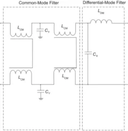
In Fig. 11 the used filter can be seen. The choice of the used components must take the real operating conditions of the filter into account. Magnetic components must be designed to avoid saturation. Moreover, insulation and ca-pacitors must be electrically strong to withstand the

occur-Fig. 12.Comparison of the measurement results with and without a filter.

ing voltages. Please note that this is only one possible fil-ter out of many different usable filfil-ter circuits. In this cir-cuit Y-capacitorsCY, common-mode chokesLCMand a

X-capacitorCXas well as a differential-mode inductorLDMare

used.

The spectrum is measured with a current measuring clamp connected to a spectrum analyzer. In Fig. 12 a comparison of the interferences on the HV-cables with and without filters is shown.

The filter attenuates the interferences in the entire required frequency range. The lower attenuation at lower frequencies can be increased by using components with lower tolerance.

6 Conclusions

In the early development process of EMC filters, simulations are helpful. Due to the large number of possible filter vari-ants, the manual determination is time-consuming. There-fore, a software tool has been developed which determines filters for DC applications quickly, efficiently and optimizes their weight, volume and cost. A further advantage is, that new filter concepts, such as hybrid filter structures can be implemented quickly and compared with conventional con-cepts. Here, an optimal filter design is determined by using a simulation tool including an effective optimization algo-rithm. The comparison of simulation and measurement re-sults show good agreement. Investigations with an electrical powertrain setup verified the filter effect.

References

Boysen, N.: Ameisenalgorithmen, 2006. Universit¨at Hamburg, 2006.

Brodersen, O. and Schumann, M.: Einsatz der Particle Swarm Opti-mization zur Optimierung universit¨arer Stundenpl¨ane, 2007, Ar-beitsbericht Nr. 05/2007. Universit¨at G¨ottingen, 2007.

DIN-EN 50178 / VDE 0160: Ausr¨ustung von Starkstromanlagen mit elektronischen Betriebsmitteln, 1998, DIN Deutsches Institut f¨ur Normung e.V. und VDE Verband deutscher Elektrotechniker e.V., 1998.

Hagmann, G.: Grundlagen der Elektrotechnik, 2008, 13 Edn., AULA-Verlag, 2008.

Marti, O and Plettl, A.: Physikalische Elektronik und Messtechnik, 2007, Universit¨at Ulm, 2007.

Rehfeld, M.: EMC-Studies for optimal Filter Design in Aircraft and Automotive Applications, 2012, Helmut Schmidt University, University of the Federal Armed Forces Hamburg, 2012. Schinkel, M.: Entwurf und Simulation aktiver EMV-Filter f¨ur

dreiphasige drehzahlver¨anderbare Antriebe, 2009, Technische Universit¨at Berlin, 2009.

Schwab, A. J. and K¨urner, W.: Elektromagnetische Vertr¨aglichkeit, 2011, 6 Edn., Springer-Verlag, 2011.

Wu, G. and Hansen, V. and Kreysa, E. and Gem¨und, H.P.: Opti-mierung von FSS-Bandpassfiltern mit Hilfe der Schwarmintel-ligenz (Particle Swarm Optimization), 2006, URSI Adv. Radio Sci., 4, 65–71, 2006,