Unifying
b
-Diversity Indices
Robert C. Szava-Kovats*, Meelis Pa¨rtel Institute of Ecology and Earth Sciences, University of Tartu, Tartu, Estonia
Abstract
Ecologists have developed an abundance of conceptions and mathematical expressions to defineb-diversity, the link between local (a) and regional-scale (c) richness, in order to characterize patterns of biodiversity along ecological (i.e., spatial and environmental) gradients. These patterns are often realized by regression ofb-diversity indices against one or more ecological gradients. This practice, however, is subject to two shortcomings that can undermine the validity of the biodiversity patterns. First, manyb-diversity indices are constrained to range between fixed lower and upper limits. As such, regression analysis ofb-diversity indices against ecological gradients can result in regression curves that extend beyond these mathematical constraints, thus creating an interpretational dilemma. Second, despite being a function of the same measureda- andc-diversity, the resultant biodiversity pattern depends on the choice ofb-diversity index. We propose a simple logistic transformation that rids beta-diversity indices of their mathematical constraints, thus eliminating the possibility of an uninterpretable regression curve. Moreover, this transformation results in identical biodiversity patterns for three commonly used classical beta-diversity indices. As a result, this transformation eliminates the difficulties of both shortcomings, while allowing the researcher to use whichever beta-diversity index deemed most appropriate. We believe this method can help unify the study of biodiversity patterns along ecological gradients.
Citation:Szava-Kovats RC, Pa¨rtel M (2014) Biodiversity Patterns along Ecological Gradients: Unifyingb-Diversity Indices. PLoS ONE 9(10): e110485. doi:10.1371/ journal.pone.0110485
Editor:Jack Anthony Gilbert, Argonne National Laboratory, United States of America
ReceivedMay 27, 2014;AcceptedSeptember 18, 2014;PublishedOctober 17, 2014
Copyright:ß2014 Szava-Kovats, Pa¨rtel. This is an open-access article distributed under the terms of the Creative Commons Attribution License, which permits unrestricted use, distribution, and reproduction in any medium, provided the original author and source are credited.
Data Availability:The authors confirm that all data underlying the findings are fully available without restriction. All relevant data are within the paper.
Funding:This study was supported by Estonian Research Council institutional research funding IUT20-29 and by the European Union through the European Regional Development Fund (Centre of Excellence FIBIR). The funders had no role in study design, data collection and analysis, decision to publish, or preparation of the manuscript.
Competing Interests:The authors have declared that no competing interests exist.
* Email: [email protected]
Introduction
Ecologists have long expressed interest in spatial and environ-mental effects on biodiversity, specifically the effects with respect to b-diversity, which quantifies the similarity of species assemblage among sites and represents the link between local (a) diversity and regional (c) diversity [1]. Consensus on a standard definition of b-diversity, however, has been elusive and has been the subject of considerable debate – both in terms of its fundamental essence [1– 5] and its mathematical relationship with a- and c-diversity [2,4,6–8]. Much mathematical discussion revolves on whether b-diversity is defined better by a multiplicative (i.e.,abM~c) [9] or
an additive (i.e.,azbA~c) [10,11] partition.
Over time, many different expressions for ‘‘b-diversity’’ have been proposed, which, in addition to considerable ambiguous terminology, has led to confusion within the ecological community [2,4,12]. Although each expression addresses the compositional similarity among sites, each is also a different measure of compositional similarity and thus, describes a somewhat different concept. The choice of beta-diversity index is, therefore, depen-dent on the researcher’s ecological application [4]. One set of beta-diversity indices, the ‘‘classical metrics’’ [1], defines a-diversity in terms of the mean a-diversity in local sites and c-diversity as the composite of these local sites.
One popular approach to quantify spatial or environmental patterns of biodiversity is regression analysis of a classical
b-diversity index against one or more spatial or environmental gradients [13–19]. This approach, however, is subject to two shortcomings that can undermine the validity of the resultant diversity patterns. First, classical b-diversity indices are mathe-matically constrained, i.e., each index features a lower limit when all local sites are compositionally the same and an upper limit when all local sites are unique. Regression of such b-diversity indices can result in a predicted estimation that crosses these limits, thus violating their mathematical constraints. Such instances cast doubt on the validity of the regression diagnostics, e.g., correlation, residuals, t-tests etc. Second, the regression analysis is dependent on the choice of b-diversity index, thus a biodiversity pattern resultant from one b-diversity index may be radically different from anotherb-diversity index.
Methods: Mathematical Properties of Logistic-Transformedb-Diversity Indices
Classicalb-diversity indices are derived from the measured local diversity (a) – usually expressed as the arithmetic mean of species richness inNlocal sites – and regional diversity (c), the measured species richness of allNlocal sites combined.b-diversity is often expressed by one of threeb-diversity indices, which are described here using the terminology in Tuomisto [4]. Trueb-diversity,bMd, expressed asc=a, quantifies the number of compositional units in
the collection. bMd is equivalent to bM, the basic multiplicative diversity partition. bMd-1, expressed as c=a{1, provides the number of complete turnovers among the compositional units in the collection. Proportional species turnover, bPt, expressed as
c{a
ð Þ=c, described the proportion of species found regionally that
are not found locally.
All three b-diversity indices, bMd, bMd-1, and bPt, assume a minimum value when all local sites are compositionally identical and a maximum when all local sites are compositionally unique. The lower limit forbMd-1andbPtis zero and forbMdunity. The respective upper limits are a function ofN(Table 1).
A logistic transformation (y~ln x=½ ð1{xÞ is a standard method by which to treat data that are constrained by upper and lower limits [20]. An analogous transformation applied to these b-diversity indices takes the generalized form, b~ln
b{bMin
ð Þ=ðbMax{bÞ
½ , wherebMaxand bMinare the respective upper and lower limit of ab-diversity index,b. Index bcan be recovered from b*
by b~expð Þ=b ½1zexpð Þb ðbMax{bMinÞz
bMin. This retransformation allows the depiction of beta-diversity in its more familiar constrained units, as a logistic variable may be difficult to visualize. The beta-diversity relationship with a gradient can be plotted simply as the retransformedb*as a function of the gradient. Any value ofb*will — upon retransformation intob— adhere to the mathematical constraint, bMinvbvbMax. Given, for example, a set ofN~10local sites with a~50 andc~100,
Table 1.Mathematical definitions and expressions of beta-diversity indices.
b-index Function Low High
bMd c=a 1 N
bMd-1 ðc{aÞ=a 0 N{1
bPt ðc{aÞ=c 0 1{ð1=NÞ
Low and High represent the lower and upper limits of beta-diversity indices as a function of the number of local sites (N).
doi:10.1371/journal.pone.0110485.t001
Table 2.Values ofc- anda-diversity along a hypothetical ecological gradient for three scenarios.
Gradient Scenario
c a(A) a(B) a(C)
1 10 9.5 2 9.5
2 20 18.6 6 10
3 40 34 6 38
4 30 18 10.5 9
5 50 37.5 17.5 31.2
6 80 24 12 46.5
7 70 21 8.4 14
8 100 12 12 40
9 80 9.6 12 24
10 90 13.5 9.9 35.8
Number of local sites (N) = 10. doi:10.1371/journal.pone.0110485.t002
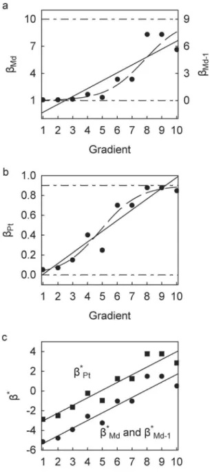
Figure 1. Scatterplots of beta-diversity indices against hypo-thetical ecological gradient for Scenario A.(a)bMd(left axis) and bMd-1(right axis); linear regression trends,bMdy~0:87x{1:17, forbMd-1
y~0:87x{2:17 (r~0:88 for both). (b) bPt; linear regression trend,
y~0:11x{0:10(r~0:95). (c)b*Md, b*Md-1 (circles) andb*Pt (squares); linear regression trends, for b*
Md b*Md-1 y~0:78x{6:10, for b*Pt
y~0:78x{3:80(r~0:91for all). Dashed trends in (a) and (b) depict linear trends ofb*Md(andb*Md-1) andb*Ptretransformed to bMd(and bMd-1) andbPt, respectively. See Table 1 for description of beta-diversity indices and Table 2 for data for Scenario A.
bMd,bMd-1, andbPtare 2, 1, and 0.5, respectively. Corresponding values of b*Md, b*Md-1, and b*Pt are 22.08, 22.08, and 0.22,
respectively. Note that because bMd{bMd-1~1, b
Md~bMd{1, and thatb
Pt~bMdzlnð ÞN ~bMd-1zlnð ÞN .
Results: Illustrative Example
Table 2 provides a set of illustrative data ofa- andc-diversity along a hypothetical environmental or spatial gradient to compare the performance of these commonly used classical b-diversity indices with their logistic-transformed equivalents. Ten points along the gradient were assigned values ofcand different values of afor three scenarios. In all scenarios,N~10, thus the upper limits forbMd,bMd-1, andbPtare 10, 9, and 0.9, respectively.
In Scenario A, bMd, bMd-1, and bPt all exhibit a statistically significant positive relationship along the gradient. The linear regression curves ofbMdandbMd-1cross below the lower limits, 1 and 0 respectively, at gradient valuesv
~
3(Figure 1a). The linear regression curve of bPt, derived from the same set ofa and c, crosses the upper limit at gradient values w~
9 (Figure 1b). In other words, Scenario A provides an example of two different b-diversity indices violating their mathematical constraints at opposite ends of the gradient. The logistic-transformed equiva-lents,b*Md, b*
Md-1, andb*
Pt, when regressed along the gradient yield statistically significant linear relationships with identical values for all regression parameters except for the intercept (Figure 1c). The intercept ofb*
Ptis 2.30 greater than that ofb*Md andb*
Md-1, which is equivalent to exp(N), i.e., exp(10). Moreover, the resultant regression curves when retransformed into their original b-diversity indices adhere to their respective upper and lower constraints (Figure 1a,b).
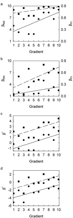
The linear regression curves ofbMd,bMd-1, andbPtin Scenarios B and C all lie within the upper and lower limits. However, the relationship between bPt and the gradient in Scenario B is statistically significant at 95% confidence (p = 0.026), whereas those between bMd and bMd-1 are non-significant (p = 0.097) (Figure 2a). This result is opposite in Scenario C: the relationship between bPt and the gradient is statistically non-significant (p = 0.121), whereas those betweenbMdandbMd-1are significant (p = 0.036) (Figure 2b). In addition, the magnitude of the residuals in Scenarios B and C differ betweenbMd(orbMd-1) andbPt. By contrast, linear regression ofb*Md, b
*
Md-1, and b *
Pt against the gradient results in identical models for both Scenario B and C with the exception of their respective intercepts. The relationship is significant for both Scenario B (p = 0.023) and Scenario C (p = 0.039) and both relationships are independent of the choice of beta-diversity index. In addition, this choice has no effect on the resultant residual patterns (Figure 2c,d).
Discussion
Space structure is an often neglected consideration in statistical analysis. All conventional multivariate statistical analysis assume that the data occupy Euclidean space [21], yet this is rarely the case. A constrained space structure can usually be readily Figure 2. Scatterplots of beta-diversity indices against
hypo-thetical ecological gradient.(a) Scenario B:bMd(circles, left axis) and bPt(squares, right axis); linear regression trends, forbMdy~0:54xz3:02
(p~0:026), for bPt y~0:02xz0:70 (p~0:097). (b) Scenario C: bMd (circles, left axis) andbPt(squares, right axis); linear regression trends, forbMdy~0:21xz1:25(p~0:121), forbPty~0:06xz1:64(p~0:036). (c) Scenario B:b*
Md(circles) andb*Pt(squares); linear regression trends,
forb*Mdy~0:29x{1:32, forb*Pty~0:29xz0:98(p~0:023for both). (d) Scenario C:b*
Md(circles) andb*Pt(squares); linear regression trends, for b*Mdy~0:36x{4:27, forb*Pty~0:36x{1:97(p~0:039for both). See Table 1 for description of beta-diversity indices and Table 2 for data for Scenario A.
transformed into Euclidean space; log-transformation of positive-only data is a well-known example. Likewise, logistic transforma-tion can be used to place data constrained by upper and lower limits into an unbounded line in Real space. Logistic transforma-tion is commonly used for data restricted to values between one and unity (as in odds ratios) [20,22], but can also be performed on constrained classicalb-diversity indices. As our illustrative example shows, regression analysis of ‘‘raw’’ classicalb-diversity indices can result in regression curves that violate their imposed mathematical constraints, thereby undermining the validity of the regression model and its interpretation. By contrast, regression of logistic-transformedb-diversity indices excludes the possibility of violating these mathematical constraints, thereby eliminating any ‘‘impos-sible’’ results that would undermine the regression model.
Logistic transformation also eliminates the effects of the choice of these classical b-diversity indices. Although regression ofbMd andbMd-1results in identical diversity patterns (the intercept using bMd-1is one less than that usingbMd), neither is equivalent tobPt, which results in a different diversity pattern. This dilemma is especially worrisome; it seems intuitive that a single measured set ofa- andc-diversity should lead to a unique diversity pattern even if b-diversity is expressed by different indices. Our illustrative example shows that a diversity pattern along an ecological gradient can be statistically significant using one index and non-significant using another. Even if the interpretational contrast is not so dramatic, the difference amongb-diversity indices can still affect the residuals, which can influence outlier detection, particularly when data points lie close to the limits. By contrast, logistic transformation results in a unique diversity pattern for all three logistic-transformed indices. The difference between b*
Md (andb*
Md-1) andb*
Ptis simply a function of the number of local sites. As a result, all regression parameters (except the intercept) are identical for allb-diversity indices.
Although the illustrative examples shown reflect simple linear regression relationships, the two advantages of the logistic transformation are maintained regardless of the actual relation-ship, i.e. even if the relationship between logistic-transformed beta-diversity and ecological gradient is markedly non-linear. As a result, the researcher is free to choose any appropriate regression model, including many non-linear models, to describe the beta-diversity pattern. For instance, a polynomial or piecewise (i.e., segmented) regression model could be used to characterize a unimodal relationship. Positive-only regression models, such as logarithmic and exponential models, are excluded, because logistic beta-diversity indices can assume negative values. The lack of equivalency among the ‘‘raw’’ classical beta-diversity indices can lead to inconsistency in describing even the qualitative nature of biodiversity patterns. For example, whereas the relationship ofbPt
with the gradient in Figure 2b is linear, the relationship withbMd andbMd-1is arguably non-linear (Figure 2a). As a result, usingbMd orbMd-1could lead to the conclusion that beta diversity increases only along the upper part of the gradient, whereas using bPt suggests that beta-diversity increases along the entire gradient.
The lack of equivalency notwithstanding, attempts to circum-vent the constraints on classical b-diversity indices by other methods are fraught with difficulty. For instance, the arc-sine transformation, despite its long tradition of use to mitigate constrained data such as percentage data, has been the subject of criticism and is rapidly running out of favour [22–24]. Moreover, the results of regression on arc-sine transformed indices remains dependent on the choice of index. Regression of logistic-transformed indices typically presumes that the data contain no regions in which all the local sites are either unique or identical; logistic transformation is impossible for a data point located exactly on an upper or lower limit. However, methods are available to perform regression analysis based on a logistic-transformed response variable that includes otherwise non-transformable data [25,26].
Although we have demonstrated the use of logistic transforma-tion on the regression of classical b-diversity indices, the transformation can also be used to circumvent violation of the constraints of pairwise ‘‘multivariate measures’’ [1], such as the Jaccard and Sørensen indices, which are constrained to values between 0 and 1. The Jaccard and Sørensen indices are equivalent tobPt and bMd-1, respectively, for a pair of sites. As such, the logistic transformation can also result in a unique diversity pattern for the Jaccard and Sørensen indices. Logistic-transformation of b-diversity indices is not limited to simple presence-absence estimates with a-diversity calculated as the arithmetic mean. A similar approach can be followed by expressinga-diversity as a geometric mean, as the maximum richness in a set of local sites [27,28], or by expressing diversity in terms of ‘‘effective numbers of species’’, which incorporates species abundance [29–31]. ‘‘Effective num-bers of species’’ can be calculated from, for instance, Shannon or Simpson indices. Moreover, the method can also be applied to phylogenetic and functional richness [32]. We suggest the logical transformation ofb-diversity indices as a means of improving and simplifying the interpretation of diversity patterns along ecological gradients.
Author Contributions
Conceived and designed the experiments: RS MP. Performed the experiments: RS. Analyzed the data: RS. Contributed reagents/materi-als/analysis tools: RS MP. Wrote the paper: RS MP.
References
1. Anderson MJ, Crist TO, Chase JM, Vellend M, Inouye BD, et al. (2011) Navigating the multiple meanings ofbdiversity: a roadmap for the practicing ecologist. Ecology Letters 14: 19–28.
2. Jurasinski G, Koch M (2011) Commentary: do we have a consistent terminology for species diversity? We are on the way. Oecologia 167: 893–902. 3. Jurasinski G, Retzer V, Beierkuhnlein C (2009) Inventory, differentiation, and
proportional diversity: a consistent terminology for quantifying species diversity. Oecologia 159: 15–26.
4. Tuomisto H (2010) A diversity of beta diversities: straightening up a concept gone awry. Part 1. Definging beta diversity as a function of alpha and gamma diversity. Ecography 33: 2–22.
5. Legendre P, De Ca´ceras M (2013) Beta diversity as the variance of community data: dissimilarity coefficients and partitioning. Ecology Letters 16: 951–963. 6. Ellison AM (2010) Partitioning diversity. Ecology 91: 1962–1963.
7. Ricotta C (2010) On beta diversity decomposition: Trouble shared is not trouble halved. Ecology 91: 1981–1983.
8. Veech JA, Summerville KS, Crist TO, Gering JC (2002) The additive partitioning of species diversity: recent revival of an old idea. Oikos 99: 3–9.
9. Whittaker RH (1960) Vegetation of the Siskiyou Mountains, Oregon and California. Ecological Monographs 30: 279–338.
10. Lande R (1996) Statistics and partitioning of species diversity, and similarity among multiple communities. Oikos 76: 5–13.
11. MacArthur R, Recher H, Cody M (1966) On the relation between habitat selection and species diversity. American Naturalist 100: 319–332.
12. Tuomisto H (2010) A consistent terminology for quantifying species diversity? Yes, it does exist. Oecologia 164: 853–860.
13. Angeler DG, Drakare S (2013) Tracing alpha, beta, and gamma diversity responces to environmental change in boreal lakes. Oecologia 172: 1191–1202. 14. Janisˇova´ M, Michalcova´ D, Bacaro G, Ghisla A (2014) Landscape effects on diversity of semi-natural grasslands. Agriculture, Ecosystems and Environment 182: 47–58.
16. Mori AS, Shiono T, Koide D, Kitagawa R, Ota AT, et al. (2013) Community assembly processes shape an altitudinal gradient of forest biodiversity. Global Ecology and Biogeography 22: 878–888.
17. Qian H, Chen S, Mao L, Ouyang Z (2013) Divers ofb-diversity along latitudinal gradients revisited. Global Ecology and Biogeography 22: 659–670. 18. Qian H, Jong-Suk S (2013) Latitudinal gradients of associations between beta
and gamma diversity of trees in forest communities in the New World. Journal of Plant Ecology 6: 12–18.
19. Rocha-Ortega M, Favila ME (2013) The recovery of ground ant diversity in secondary Lacandon tropical forests. Journal of Insect Conservation 17: 1161– 1167.
20. Bolker BM (2008) Ecological Models and Data in R. Princeton, NJ: Princeton University Press. 396 p.
21. Bacon-Shone J (2011) A short history of compositional data analysis: Theory and Applications. In: V Pawlowsky-Glahn and A Buccianti, editors.Compositional Data Analysis.West Sussex: John Wiley & Sons, Ltd. pp.3–11.
22. Wilson K, Hardy CW (2002) Statistical analysis of sex ratios: an introduction. In: I. C. W Hardy, editor editors.Sex Ratios: Concepts and Research Methods. Cambridge: Cambridge University Press. pp.48–92.
23. Milligan GW (1987) The use of the Arc-Sine Transformation in the Analysis of Variance. Educational and Psychological Management 47: 563–573.
24. Warton DI, Hui FKC (2011) The arcsine is asinine: the analysis of proportions in ecology. Ecology 92: 3–10.
25. Papke LE, Wooldridge JM (1996) Econometric methods for fractional response variables with an application to 401(k) plan participation rates. Journal of Applied Economoetrics 11: 619–632.
26. Ramalho EA, Ramalho JJS, Murteira JMR (2011) Alternative estimating and testing empirical strategies for fractional regression models. Journal of Economic Surveys 25: 19–68.
27. Harrison S, Ross SJ, Lawton JH (1992) Beta diversity on geographic gradients in Britain. Journal of Animal Ecology 61: 151–158.
28. Magurran AE (2004) Measuring Biological Diversity.. Oxford: Blackwell Publishing. 256 p.
29. Hill MO (1973) Diversity and evenness: a unifying notation and its consequences. Ecology 54: 427–432.
30. Jost L (2006) Entropy and diversity. Oikos 113: 363–375.
31. Jost L (2007) Partitioning diversity into independent alpha and beta components. Ecology 88: 2427–2439.