www.scielo.br/cam
Exact solutions for drying with coupled phase-change
in a porous medium with a heat flux condition
on the surface
EDUARDO A. SANTILLAN MARCUS and DOMINGO A. TARZIA
Depto. de Matemática and CONICET, FCE, Universidad Austral Paraguay 1950, S2000FZF Rosario, Argentina
E-mails: [email protected] / [email protected]
Abstract. Exact solutions for the problem of drying with coupled phase change in a porous
medium with a heat flux condition onx=0 of the type−q0/√τ ,withq0>0, for any value of
the Luikov numberLuis obtained. This solution can be only obtained whenq0verifies a certain
inequality. Besides, for large Luikov number
more precisely,Lu >
1
εK0+1
, we obtain
that the temperature distributiont2reaches to a minimum value which is smaller than its initial
temperature or limit value reached at+∞.
Mathematical subject classification:35R35, 80A22, 35C05.
Key words: free boundary, Stefan problem, phase change, drying, heat conduction, mass
transfer, porous medium.
1 Introduction
Heat and mass transfer with phase change problems, taking place in a porous medium, such as evaporation, condensation, freezing, melting, sublimation and desublimation, have wide application in separation processes, food technology, heat and mixture migration in soils and grounds, etc. Due to the non-linearity of the problem, solutions usually involve mathematical difficulties. Only a few exact solutions have been found for idealized cases. Mathematical formulation of the heat and mass transfer in capillary porous bodies has been established by Luikov [13], [14], [15], [16], [17]. Other problems in this direction are [3], [6], [7], [9], [20], [22].
A large bibliography on free and moving boundary problems for the heat-diffusion equation was given in [23]. Gupta [10] presented an approximate solution to a coupled heat and mass transfer problem involving evaporation. The problem Gupta [10] treated has analytical solution, which is presented in Cho [5]. Heat and mass transfer during drying from an homogeneous point of view are also considered in [1], [2], [4], [8], [11], [18], and [19].
In the following, we study a similar problem as that of [5]. A semi-infinite porous medium is dried by maintaining a heat flux condition atx = 0 of the type −q0/
√
t , with q0 > 0, which was firstly considered in [21]. Initially,
the whole body is at uniform temperature t0 and uniform moisture potential u0.The moisture is assumed to evaporate completely at a constant temperature,
evaporation pointtv. It is also assumed that the moisture potential in the first region, 0< x < s (τ ) ,is constant atuv,wherex =s (τ )locates the evaporation front at timeτ >0. It is further assumed that the moisture in vapor form does not take away any appreciable amount of heat from the system. Neglecting mass diffusion due to temperature variation, the problem can be expressed as:
∂t1
∂τ (x, τ )=a1 ∂2t1
∂x2 (x, τ ) , 0< x < s (τ ) , τ >0 (region 1) (1.1) u1=uv, 0< x < s (τ ) , τ >0 (region 1) (1.2) ∂t2
∂τ (x, τ )=a2 ∂2t
2 ∂x2 +
εLcm c2
∂u2
∂τ , x > s (τ ) , τ >0 (region 2) (1.3)
∂u2
∂τ (x, τ )=am ∂2u
2
∂x2 (x, τ ) , x > s (τ ) , τ >0 (region 2) (1.4)
The initial and boundary conditions are:
k1 ∂t1 ∂x = −
q0
√
τ at x =0, τ >0 (1.5)
u1(s (τ ) , τ )=u2(s (τ ) , τ )=uv< u0 at x =s (τ ) (1.9)
−k1 ∂t1
∂x (s (τ ) , τ )+k2 ∂t2
∂x (s (τ ) , τ )=(1−ε) ρmL ds dt
at x =s (τ )
(1.10)
Symbols are given in the nomenclature. We clarify thatt1is the temperature
of the dried porous medium,t2is the temperature of the humid porous medium
andu2is the mass-transfer potential of the humid porous medium.
In paragraph 2, we find a solution of this problem, depending on the value of the Luikov numberLu, then in paragraphs 3 and 4 we discuss the equation that determines the dimensionless constant which characterizes the evaporation front when the Luikov numberLuequals to one andLuis different to one. Finally, in paragraph 5 we give some illustrative results and a sufficient condition (5.4) for the Luikov numberLuin order to obtain when the temperature distribution has a minimum value less than its initial temperature.
This study was motivated by the following mathematical and physical analysis. Taking into account (1.1), (1.5) and (1.8), and (1.4), (1.7) and (1.9), by the maximum principle, we havet1(x, τ ) > tvfor region 1 anduv< u2(x, τ ) < u0
for region 2 respectively. We expect from a physical point of view that the phase change fronts (τ ) should be an increasing function. In this case, thanks again
to the maximum principle, we should obtain that ∂u2
∂τ (x, τ ) < 0 for region
2, then the heat equation (1.3) has a heat sink within the corresponding region 2. Due to the maximum principle, we havet2(x, τ ) < tv for region 2 and we
can say anything about where the temperature has an absolute minimum value. One of the goals of this paper is to obtain a sufficient condition for the data in order to have a minimum value for the temperature within its corresponding domain. Moreover, we can characterize the coordinate of this point when the dimensionless variable η = x
2√a1τ
takes the value (5.7) as a function of the
2 Solution of the problem
Let be the following dimensionless variables and parameters:
Ui = ui −u0
uv−u0
, fori =1,2 (2.1)
Ti = ti −t0
tv−t0
, fori =1,2 (2.2)
η= x
2√a1τ
(2.3)
Lu = am
a1
>0 (2.4)
Ko= Lcm(u0−uv)
c2(tv−t0)
>0 (2.5)
ν= (1−ε) ρmLa1
k1(tv−t0)
>0 (2.6)
k21= k2 k1
>0. (2.7)
AssumingUandT are only functions of the variableη, the conditions (1.1)-(1.9) imply us that
s (τ )=2λ√a1τ (2.8)
where λ is a positive constant to be determined later. Therefore, equations (1.1)-(1.4) are transformed to the following dimensionless ordinary differential equations of the form:
T1′′(η)+2ηT1′(η)=0, 0< η < λ (2.9)
U1=1, 0< η < λ (2.10)
T2′′(η)+2ηT2′(η)−2εKoηU2′(η)=0, η > λ (2.11)
The boundary conditions (1.5)-(1.10) become:
T1′ = − 2q0
√
a1 k1(tv−t0)
at η=0, (2.13)
T2 =0 as η→ ∞, (2.14)
U2=0 as η→ ∞, (2.15)
T1=T2=1 at η=λ, (2.16)
U1=U2=1 at η=λ, (2.17)
T1′−k21T2′= −2νλ at η=λ, (2.18)
Solutions of the equations (2.9) and (2.12), which satisfy boundary conditions (2.13), (2.15), (2.16) and (2.17), are easily obtained as follows
T1(η)=1+
q0√π a1 k1(tv−t0)
(erfλ−erfη) , 0< η < λ (2.19)
U2(η)=
1−erf
η
√
Lu
1−erf
λ
√
Lu
, η > λ. (2.20)
Substituting expression (2.20) into equation (2.11), and solving the result-ing non-homogeneous ordinary differential equation with boundary conditions (2.14) and (2.16), we obtain the following results, depending on Lu = 1 or
Lu=1,i.e.:
T2(η) =
εKo
√
π (1−erf(λ))
λ e−λ21−erf(η)
1−erf(λ) −η e
−η2
+1−erf(η)
1−erf(λ), if Lu =1, η > λ
or
T2(η) =
εKoLu Lu−1
−
1−erf√η
Lu
1−erf
λ
√
Lu +
1−erf(η)
1−erf(λ)
+1− erfη
1−erfλ, if Lu=1, η > λ.
(2.22)
Functions (2.19), (2.20) and (2.21) or (2.22) satisfy all boundary conditions except condition (2.18). Substituting these expressions into condition (2.18), the positive constantλis determined from the following equation, depending on the value ofLu,as follows:
k21
√
π
e−λ2
1−erf(λ)
−2√εK0
π λ e−λ2
1−erf(λ) +2εK0λ 2
−εK0−2
+ 2 √a
1q0 k1(tv−t0)
e−λ2 =2νλ, λ >0 if Lu =1,
(2.23)
or
√π a
1q0 (tv−t0)
e−λ2+ LuεK0
Lu−1k2
1
√
LuF1
λ
√
Lu
−F1(λ)
= k2F1(λ)+
√
π k1νλ, λ >0 if Lu =1.
(2.24)
3 Discussion of the equation that determinesλ, considering the case when the Luikov number equals to one
Now let’s study in detail the equation (2.23), vinculated to the caseLu=1,that is to say, whenam=a1.We define the following real functions:
α (x) =√k21 π
e−x2
1−erf(x)
−2√εK0
π x
e−x2
1−erf(x)+2εK0x
2
−εK0−2
+ 2
√a
1q0
k1(tv−t0)
e−x2
(3.1)
Then, equation (2.23) can be expressed saying thatλmust be the solution of the following equation
α (x)=χ (x) , x > 0. (3.3)
We shall see the characteristics of each one of the functions α and χ which appears in equation (3.3).
Firstly, we have thatχis a strictly increasing function, with the properties:
χ (0)=0; χ (+∞)= +∞ ; χ′(x)=2ν >0, x >0.
Before we study the functionα, let’s define the following real functions:
Q (x)=√π xe−x2(1−erf(x)) , x >0
W (x)= √x π
e−x2
1−erf(x) −x 2
=x2
1
Q (x)−1
, x >0.
FunctionQhas the following properties:
Q0+=0; Q (+∞)=1; Q′(x) >0, x >0.
FunctionW is a positive valued function, with the following properties [12]:
W0+=0; W (+∞)= 1
2; W
′(x) >0
thenW is a strictly increasing function. Now we take care aboutα. Taking into accountW,we can putαin the following way:
α (x)= 2 √a
1q0 k1(tv−t0)
e−x2 −√k21
πF1(x)
2εK0W (x)+εK0+2
where functionF1is defined by
F1(x)=
e−x2
1−erf(x) (3.4)
which has the following properties
F1
0+
lim
x→+∞ F1(x)
x =
√
π Q (+∞) =
√
π .
Thenα is written as the sum of two strictly decreasing functions, therefore it results that α is also a strictly decreasing one. Besides, it has the following properties:
α (0) = 2 √
a1q0 k1(tv−t0)
−√k21
π [εK0+2]; α (+∞)= −∞
α′(x) = −4x √a
1q0 k1(tv−t0)
e−x2 −√k21
π
e−x2
1−erf(x)
2εK0W′(x)
+ (−√k21)
π F
′
1(x)
2εK0W (x)+εK0+2
<0, x >0.
Next, to assure that the two functionsα andχ have an intersection point, we need to assume that
α (0) > χ (0) ,
that is to say, 2
√a
1q0 k1(tv−t0)
> √k21
π [εK0+2],which is equivalent to the condition q0>
k2(tv−t0)
2√π a1
εK0+2
, (3.5)
and we can finally give the following:
Theorem 3.1. If the Luikov number is equals to one, and the coefficient q0
verifies the condition(3.5) then there exists one and only one solutionλ > 0 of the equation(2.23). Furthermore, the solution of the problem(1.1)-(1.10)
is given by(2.19)-(2.21), whereλis the unique solution of the equation(2.23), that is:
u1(x, τ )=uv, 0< x < s (τ ) , τ >0 (3.6)
t1(x, τ ) =1+
q0√π a1 k1(tv−t0)
erfλ−erf
x
2√a1τ
,
0< x < s (τ ) , τ >0
u2(x, τ )=
1−erf
x
2√amτ
1−erf(λ) , x > s (τ ) , τ >0 (3.8)
t2(η) =
εK0
√
π (1−erf(λ))
λ e−λ2
1−erf
x
2√a1τ
1−erf(λ) − x
2√a1τ e− x
2 4a1τ
+
1−erf
x
2√a1τ
1−erfλ , x > s (τ ) , τ >0 (3.9)
s (τ )=2λ√a1τ . (3.10)
4 Discussion of the equation that determinesλ, considering the case when the Luikov number is different to one
In this paragraph we will study in detail the equation (2.24), which determines the unknownλfor the caseLu =1,that is to say,am=a1.For this propose, we
define the following functions:
φ (x)=
√
π a1q0 (tv−t0)
e−x2+P (x) (4.1)
ϕ (x)=k2F1(x)+
√
π k1νx. (4.2)
where
P (x)= LuεK0
Lu−1k2
1
√
LuF1
x
√
Lu
−F1(x)
, x >0. (4.3)
Then, equation (2.24) can be written saying thatλmust be the solution of the equation
φ (x)=ϕ (x) , x >0. (4.4)
Firstly, let’s see thatϕ (x)is a strictly increasing function with the properties:
ϕ (0)=k2; ϕ (+∞)= +∞ ; ϕ′(x) >0, x >0.
Before studyingφ, we need to analyse the functionP. Obviously, functionP whenx =0+ is equal to−√√LuεK0
Lu+1 k2 <0, and when xtends to+∞its behaviour may depends on the value ofLu.Well, it doesn’t happen: We have lim x→∞ F1 x √ Lu
F1(x) − Lu = 1 √ Lu −
Lu = 1√−Lu
Lu ,
so, we can verify that:
i) If Lu > 1, we have lim
x→∞
1
√
LuF1
x
√
Lu
−F1(x)
= −∞, then
P (+∞)= −∞.
ii) If Lu < 1, we have lim
x→∞
1
√
LuF1
x
√
Lu
−F1(x)
= +∞, then
P (+∞)= −∞.
Therefore, it doesn’t matter whetherLuis less or greater than 1,P (x)always tends to−∞whenx → +∞. Then, the properties ofφ (x)are:
φ (0)=
√π a
1q0
(tv−t0)+
P
0+
= √π a
1q0
(tv−t0)−
√
LuεK0
√
Lu+1
k2; φ (+∞)= −∞
φ′(x)= −2
√π a
1q0
(tv−t0)
xe−x2+LuεK0 Lu−1
k2
1
Lu
F1′
x
√
Lu
−F1′(x)
<0, x >0.
Concluding, to assure an intersection point between the two functionsφ and
ϕ,we impose the conditionφ (0) > ϕ (0) ,that is to say
√π a
1q0 (tv−t0) −
√
LuεK0
√
Lu+1k2> k2, which is equivalent to
q0> k2
1+
√
LuεK0
1+√Lu
tv−t0
√
π a1
, (4.5)
Theorem 4.1. If the Luikov number is different than one, and the coefficientq0
verifies the condition(4.5) then there exists one and only one solutionλ > 0 of the equation(2.24). Furthermore, the solution of the problem(1.1)-(1.10)is given by(2.19)-(2.21), whereλis the solution of the equation(2.24), that is:
(3.6),(3.7),(3.8),(3.10)and
t2(η) =
εKoLu Lu−1
−
1−erf
x
2√amτ
1−erf
λ
√
Lu +
1−erf
x
2√a1τ
1−erf(λ)
+
1−erf
x
2√a1τ
1−erfλ , x > s (τ ) , τ >0.
(4.6)
Remark 1. The right side member of the inequality (4.5) goes to the right side member of the inequality (3.5) whenLutends to 1,that is to say, we can study the caseLu =1 considering the limitLu →1 in the caseLu =1,then we can resume both results in the following one:
Theorem 4.2. Let be consider the coefficientq0verifying the condition(4.5),
then, for any positive value ofLu,there exists one and only one solutionλ >0of the equation(2.23)or(2.24)depending on what value takesLu. Furthermore, the solution of the problem(1.1)-(1.10)is given by:
a) (3.7)-(3.8),(3.9) and(3.10), if Lu =1,
b) (3.7)-(3.8),(4.6) and (3.10), if Lu =1.
5 Some illustrative results and a sufficient condition for the Luikov number in order to obtain the minimum value of the temperature distribution
Some results of sample calculations are shown here. In this examples we take
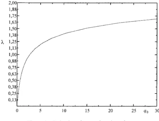
εK0=2, a1=1, k2=1,and(tv−t0)=1.Figure 1 shows the behaviour ofλ
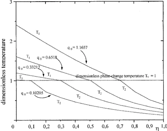
as a function ofq0.Figure 2, 3 and 4 shows the behaviour of the dimensionless
Figure 1 – Behavior ofλas a function ofq0.
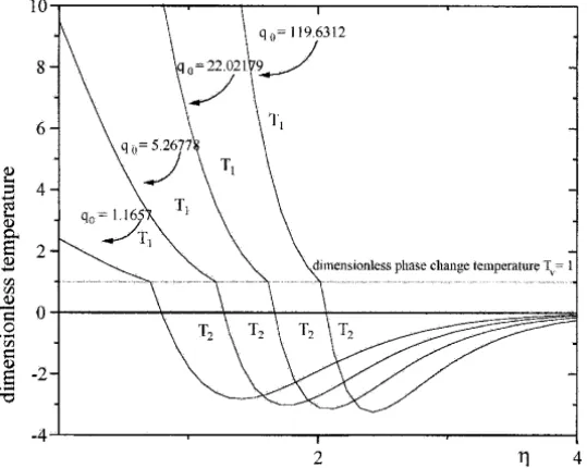
Looking at Figures 2, 3 and 4, we see that the temperature distribution t2
reaches to a minimum value which is smaller than the limit valuet0 that the
function reaches at+∞, i.e. the initial temperature, although in Figure 2 the function has no such minimum value. We shall find the values of the coefficient
Lufor which the functionT2has a minimum value which is smaller than its limit
value whenη→ +∞.
ForLu=1, we takeT2(η)for anyη > λ, and we have
T2′(η)= εKoLu
Lu−1
2
√
π Lue
−Luη2
1−erf
λ
√
Lu −
2
√
π e(
−η2)
1−erf(λ)
−
2
√
π e(
−η2)
1−erfλ
and we get that
T2′(η) = 0 ⇔ εKo √
Lu Lu−1
e
− η2 Lu
1−erf
λ
√
Lu =
εKoLu Lu−1 +1
e(−η2)
1−erfλ
Figure 2 – Behavior of the temperature with respect to the dimensionless variableη
consideringLu=0.1<1.
Figure 3 – Behavior of the temperature with respect to the dimensionless variableη
Figure 4 – Behavior of the temperature with respect to the dimensionless variableη
consideringLu=4>1.
S (x)=Z (x) , x > λ, (5.1)
whereSandZare defined by:
S (x)= εKo
√
Lu Lu−1
e − x2 Lu
1−erf
λ
√
Lu
(5.2)
Z (x)=
εKoLu Lu−1 +1
e(−x2)
1−erfλ (5.3)
Obviously, bothSandZare strictly decreasing (increasing) functions for any
x >0 whenLu>1 (0< Lu <1). Moreover, we have
S (x)=Z (x)⇔ εKoLu e − x2 Lu
1−erf
λ
√
Lu
=((εK0+1) Lu−1)
e(−x2)
1−erfλ
⇔ e
1−Lu1 x2
= ((εK0+1) Lu−1)
εKo√Lu
1−erf
λ
√
Lu
1−erfλ
which implies that in order to solve the equation (5.1), firstly we must to assume that((εK0+1) Lu−1) >0,that is
Lu> 1 εK0+1
(5.4)
Secondly, ifLu >1 we must to impose that
((εK0+1) Lu−1) εKo√Lu
1−erf
λ
√
Lu
1−erfλ >1 (5.5)
which is always satisfied taking into account that the error function is a strictly increasing function. Moreover, ifLu <1 we must to impose that
((εK0+1) Lu−1) εKo√Lu
1−erf
λ
√
Lu
which is satisfied for all 0< Lu <1. Therefore, if the Luikov numberLuverifies the condition (5.4) we obtain that the solution of the equationS(x) =Z(x)is given by
η=
Lu Lu−1
log
((εK0+1) Lu−1) εKo√Lu
1−erf
λ
√
Lu
1−erfλ
(5.7)
Then we have obtained the following result:
Theorem 5.1. If the Luikov numberLuverifies the condition(5.4)the temper-ature distributiont2reaches to a minimum value which is smaller than the initial
temperature or its limit value at+∞. The minimum value is attained when the dimensionless variableηtakes the value(5.7).
Remark 2. For large Luikov number the temperature distributiont2 = t2(η)
has an absolute minimum value less than its initial temperature. Moreover, the minimum value for the Luikov number in order to have that property is given
explicitely by the coefficient 1
εK0+1
,which is not an intuitive result.
6 Conclusion
Exact solutions for the problem of drying with coupled phase change in a porous medium with a heat flux condition onx = 0 of the type −√q0
τ, withq0 > 0,
for any value ofLuis obtained. This solution is only obtained whenq0verifies
a certain explicited inequality. The temperatures of the two phases and the mass-transfer potential were obtained by using the similarity method. Some illustrative results are shown. Finally, for large Luikov numbermore precisely,
Lu > 1 εK0+1
we obtain that the temperature distribution t2 reaches to an
absolute minimum value which is smaller than the initial temperature (or its limit value at+∞), and we characterize the coordinate of this point when the dimensionless variable η = x
2√a1τ
takes the value (5.7) as a function of the
7 Acknowledgments
This paper has been partially sponsored by the project ‘‘Free Boundary Problems for the Heat-Diffusion Equation’’ from CONICET-UA, Rosario (Argentina) and ‘‘Partial Differential Equations and Numerical Optimization with Applications’’ from Fundación Antorchas (Argentina).
Nomenclature:
ai, i=1,2 thermal diffusivity of the phase-i.
a12 ratio of thermal diffusivities from phase 1 to phase 2
am moisture diffusivity
cm specific mass capacity
c2 specific heat capacity
ki, i =1,2 thermal conductivity of the phase-i.
k21 ratio of thermal conductivity from phase 2 to phase 1 K0=
Lcm(u0−uv) c2(tv−t0)
Kossovitch number
L latent heat of evaporation of liquid per unit mass
Lu=ama1 Luikov number
q0 coefficient that characterizes the heat flux atx =0 s(τ ) position of the evaporation front
ti(x, τ ), i=1,2 temperature of the phase-i.
t0 initial temperature
tv temperature at the phase-change state
Ti, i =1,2 non-dimensional temperature of the phase-i
u mass-transfer potential
u0 initial mass-transfer potential
Ui, i =1,2 dimensionless mass-transfer potential of the phase-i
x space coordinate
Greek symbols
ε coefficient of internal evaporation
η dimensionless variable
λ dimensionless constant which characterizes the evaporation front
ρm density of moisture
τ time
Subscripts
0 at initial time,t=0
1 dried porous medium,0< x < s (τ )
2 humid porous medium, x > s (τ ) v at evaporation front,x=s (τ )
REFERENCES
[1] A. Ali Cherif, A. Daïf,Etude numérique du transfert de chaleur et de masse entre deux plaques planes verticales en présence d’un film de liquide binaire ruisselant sur l’une des plaques chauffée, Int. J. Heat and Mass Transfer42(1999), 2399–2418.
[2] Y. Le Bray and M. Prat,Three-dimensional pore network simulation of drying in capillary porous media, Int. J. Heat and Mass Transfer42(1999), 4207–4224.
[3] H.S. Carslaw and J.C. Jaeger,Conduction of heat in solids, Clarendon Press, Oxford, (1959).
[4] J. Chen and J. Lin,Thermocapillary effect on drying of a polymer solution under non-uniform radiant heating, Int. J. Heat and Mass Transfer43(2000), 2155–2175.
[5] S.H. Cho,An exact solution of the coupled phase change problem in a porous medium, Int. J. Heat and Mass Transfer18(1975), 1139–1142.
[6] S.H. Cho and J.E. Sunderland,Heat conduction problem with melting or freezing, J. Heat. Transfer91(1969), 421–426.
[7] A. Fasano, M. Primicerio and D.A. Tarzia,Similarity solutions in class of thawing processes, Math. Models Methods Appl. Sci.,9(1999), 1–10.
[8] C. Figus, Y. Le Bray, S. Bories and M. Prat,Heat and mass transfer with phase change in a porous structure partially heated: continuum model and pore network simulations, Int. J. Heat and Mass Transfer42(1999), 2557–2569.
[10] L.N. Gupta,An approximate solution to the generalized Stefan’s problem in a porous medium, Int. J. Heat Transfer17(1974), 313–321.
[11] J. Häger, M. Hermansson and R. Wimmerstedt,Modeling steam drying of a single porous ceramic sphere: experiments and simulations, Chem. Eng. Sci.52(1997), 1253–1264.
[12] A.L. Lombardi and D.A. Tarzia,Similarity solutions for thawing processes with a heat flux condition at the fixed boundary, Meccanica,36(2001), 251–264.
[13] A.V. Luikov,Heat and mass transfer in capillary-porous bodies, Adv. Heat Transfer1(1964), 123–184.
[14] A.V. Luikov,Heat and mass transfer in capillary-porous bodies, Pergamon Press, Oxford, (1966).
[15] A.V. Luikov,Analytical heat diffusion theory, Academic Press, New York, (1968).
[16] A.V. Luikov,Systems of differential equations of heat and mass transfer in capillary porous bodies, Int. J. Heat Mass Transfer18(1975), 1–14.
[17] A.V. Luikov,Heat and mass transfer, MIR Publishers, Moscow, (1978).
[18] A. Mhimid, S. Ben Nasrallah, J.P. Fohr,Heat and mass transfer during drying of granular products – simulation with convective boundary conditions, Int. J. Heat and Mass Transfer
43(2000), 2779–2791.
[19] P. Perré and I.W. Turner,A 3-D version of TransPore: a comprehensive heat and mass transfer computational model for simulating the drying of porous media, Int. J. Heat and Mass Transfer42(1999), 4501–4521.
[20] E.A. Santillan Marcus and D.A. Tarzia,Explicit solution for freezing of humid porous half-space with a heat flux condition, Int. J. Eng. Sci.38(2000), 1651–1665.
[21] D.A. Tarzia,An inequality for the coefficientσ of the free boundarys(t ) = 2σ√tof the Neumann solution for the two-phase Stefan problem, Quart. Appl. Math.39(1981), 491-497.
[22] D.A. Tarzia,Soluciones exactas del problema de Stefan unidimensional, Cuadern. Inst. Mat. B. Levi12(1985), 5-36.