A mathematical model for virus infection in a
system of interacting computers
J. LÓPEZ GONDAR and R. CIPOLATTI
Departamento de Matemática Aplicada
Instituto de Matemática, Universidade Federal do Rio de Janeiro C.P. 68530, Rio de Janeiro, Brasil
E-mail: [email protected] / [email protected]
Abstract. We introduce a simplified theoretical model to describe a virtual virus propagation process in a set of interacting computers. The propagation mechanisms considered here are those related to the reception of messages through internet as well as the ones concerning the simple exchange of files using recording devices as compact disks or the commonly used floppy disks. In spite of its inherent simplicity, this model provides a good idea of the infection process and trends. From the mathematical point of view, the nonlinear delay integral equation that we obtain here presents certain interesting features which are explored and enlightened in this paper.
Mathematical subject classification:45G10, 49K25, 92D99.
Key words:virtual viruses, nonlinear delay integral equation.
1 Introduction
The infection of computers by virtual viruses is a present day problem. A lot of efforts have been (and will be) devoted to the development of virtual vaccines each time a new virus appears. Nevertheless, slow progress (if any) in understanding the propagation process, quantitatively, has been obtained up to now. In a certain sense, the propagation of virtual viruses in a system of interacting computers could be compared with a disease transmitted by vectors when dealing with public health. Concerning diseases transmitted by vectors, one has to take into account that the parasite spends part of its lifetime inhabiting the vector, so that the infection switches back and forth between host and vector. Almost the same
occurs here and also a certain time interval elapses between successive contacts which, in this case, involves an electronic message (or a recording device) and two different computers. However, we have to point out that, in our simplified model, which ignores finer details, we suppose in the case of recording devices that they are simple carriers not permanently infected, which could transmit the virus only once (if it is so); i.e., after the first transmission of a certain program, the contents in the recording device are removed before it is used again. Under such hypothesis (among others considered below) we obtain a compact model restricted to one single integral equation.
The paper is organized as follows: in Section 2, we construct the theoretical model. Section 3 is devoted to performing a mathematical analysis of the in-tegral equation obtained: existence, uniqueness and asymptotic behavior of the solutions, as well as stability of stationary solutions. Finally, Section 4 contains numerical experiments and our conclusions.
2 Modeling the dynamics of transmission
Before introducing the new model to describe the way by which some virtual virus infection transmitted by electronic messages (or by recording devices) could spread through a population of computers as a function of time, we shall start deducing a certain contact-propagation equation for a general infectious process having a natural (or induced) recovering time. We consider such an equation as a convenient point of reference for subsequent analysis. In the present approach we shall assume to deal with a new kind of virus infection for which there exists no vaccine available. Being so, the unique way to restore the functions of an infected computer is by deleting the hard disk (with which it becomes susceptible again). It should be pointed out that neither spatial dependence nor latent periods or immunity factors will be considered here.
Therefore, the total population is divided into two classes:
(S) the susceptible class; i.e., those individuals capable of contracting the disease, becoming themselves infected.
The closed host population of total sizeN will be used as a normalization factor, so we setI +S=1.
Let us denote byg(τ )the rate of the infection process at timeτ, i.e., the number of new infected computers (population density of them) per unit time, at instant τ. We also introduce a function of two variablesP (t, τ ),P:→ [0,1], where
=(t, τ )∈R2; t≥τ, (2.1)
which represents the probability of a computer infected atτ to remain infectious at t. Such a function, of course, is related to the time elapsed between the detection of the infection and its eradication by erasing the hard disk. Considering a maximum recovering time T, the function P (t, τ ) is supposed to have the following general properties:
i) P (t, τ )=1 if τ =t; ii) P (t, τ )=0 if τ ≤t−T;
iii) P (t, τ ) is a monotone decreasing function oftfor each fixedτ. (2.2)
If we want to describe the density of infective individuals as a function of time, starting att =0, the only infected ones to be considered should be those in the interval[−T , t](just because of the maximum recovering timeT).
Dividing this interval intonequal parts, so thatτ =(t+T )/nand defining τ1= −T,τ2= −T+τ, . . . , τn+1= −T+nτ, i.e.,τj = −T+(j−1)τ,
j = 1, . . . , n+1, we should state, forτ small enough, that the number of infected individuals in the interval[τj, τj+1] = [τj, τj +τ]is given,
approxi-mately, as
g(τj)(τj+1−τj)=g(τj)τ, j =1,2, . . . , n. (2.3)
Then, the number of infected individuals in this interval which remain infective att is approximately,
and therefore, the total number of infective individuals at t may be written, approximately, as
n
j=1
g(τj)P (t, τj)τ, (2.5)
which, in the limitτ →0, gives
I (t )=
t
−T
g(τ )P (t, τ ) dτ, t≥0. (2.6)
Taking into account thatP (t, τ )=0 ifτ ≤t−T, we should write Eq. (2.6) as
I (t )=
t
t−T
g(τ )P (t, τ ) dτ, t≥0. (2.7)
The former equation contains the basic features for the evolution of an infection process in the framework of a SIS model. Depending on the specific transmission process, one should conceive, in each case, a suitable infection rate-functiong(τ ). As it can be verified in references [4, 6], Eq. 2.7 and variations of it have already been used by other authors in describing the propagation of diseases.
Concerning the propagation of virtual viruses transmitted by electronic mes-sages (a) or by recording devices (b), we shall establish the following hypothesis to constructg(τ ):
a) some finite time elapses between the act of sending and the reception of messages (t0on average);
b1) each recording device is used only twice in intervals of timet0, on average; b2) each device transmits the infection when, used by the first time in an infected computer, it is used by the second time in a susceptible one. Once this process occurs, previous contents are deleted.
Event Probability
I →I I (t )I (t +t0)
S→S S(t )S(t +t0)=
1−I (t )1−I (t+t0)
I →S I (t )S(t+t0)=I (t )
1−I (t+t0)
S →I S(t )I (t0)=
1−I (t )I (t+t0) Among them we are only interested in the third one.
By a direct calculation, one can easily verify that the sum of the above proba-bilities gives just 1.
Of course, there exists some characteristic average frequency for the submis-sion of electronic messages in the system of interacting computers considered here, as well as recording devices are subjected to a certain recording frequency. We shall denote such a characteristic frequency byNr(t ). Then, for a time
in-tervalt small enough, we may write the number of new infected computers which are increased to those already existing att+t0, approximately, by
NI|t+t0 =Nr(t )t I (t )
1−I (t+t0)
. (2.8)
Dividing byN tand taking the limit ast→0, we have
g(t+t0)= Nr(t )
N I (t )
1−I (t+t0)
. (2.9)
If we make the substitutiont→t+t0, Eq. (2.9) may be written as g(t )= Nr(t−t0)
N I (t−t0)
1−I (t ), (2.10)
or
g(t )=α(t )I (t−t0)
1−I (t ), (2.11)
where
α(t )= Nr(t−t0)
Therefore, in the framework of our model and following Eq. (2.7), the density of infective computers at timetdue to the virtual virus propagation process obeys the following law
I (t )=
t
t−T
α(τ )I (τ−t0)
1−I (τ )P (t, τ ) dτ, t >0, (2.13)
whereα(τ )is given by (2.12).
Eq. (2.13) is a delay integral equation and the existence of solutions fort≥0 depends on data defined in the past−T −t0≤t ≤0.
Although we are only consideringt0 >0, it is interesting to point out that, if t0=0 andP (t, τ )=φ (t−τ ), whereφ (ξ )is a real function, Eq. (2.13) reduces to the special case considered by Cooke and Yorke in [6].
3 Existence, uniqueness and asymptotic behavior
In this section we consider the problem of existence, uniqueness and asymptotic behavior of solutions for equation (2.13). We will say that a functionI (t )is a solution generated by I0 ifI (t ) = I0(t ) a.e. in[−T −t0,0] and if I (t ) also satisfies (2.13) fort >0.
• Uniqueness:
We consider the setdefined by (2.1), a functionP: → [0,1]such that (2.2) holds andI0∈L∞
−T −t0,+∞
.
In order to avoid technicalities (see Remark 3.2), we assume that
α∈C[−T −t0,+∞ [
. (3.1)
Lemma 3.1. Assume thatαsatisfies(3.1). IfI1andI2are solutions of(2.13) generated byI0(t ), thenI1(t )=I2(t )for allt >0.
Proof. First of all it should be noticed that, ifIi is a solution of (2.13), thenIi
is continuous in]0,+∞ [. For 0< t ≤t0we have
I1(t )−I2(t )=
t
t−T
α(τ )I0(τ−t0)
I2(τ )−I1(τ )
Letϕbe the function defined byϕ(t )= |I1(t )−I2(t )|. Since 0≤P (t, τ )≤1, it follows that
ϕ(t )≤ I0
t
0
|α(τ )|ϕ(τ ) dτ, 0< t ≤t0, (3.2) whereI0 =ess sup|I0(τ )| ; −T −t0≤τ ≤0
. Defining
ψ (t )=
t
0
|α(τ )|ϕ(τ ) dτ,
it follows thatψis differentiable in]0,+∞[and we haveψ′(t )= |α(t )|ϕ(t ). After multiplying both sides of (3.2) by|α(t )|, we get
ψ′(t )− I0|α(t )|ψ (t )≤0, 0< t < t0, from which we obtain
d dt
ψ (t )exp
−I0
t
0
|α(τ )|dτ ≤0, 0< t < t0.
Sinceψ (0)=0, we conclude thatψ (t )=0 as well asϕ(t )=0 for all 0< t ≤t0. The same arguments can be repeated for(k−1)t0 < t ≤ kt0, for allk∈ N,
and the proof is achieved.
Remark 3.2. We can obtain the same result of Lemma 3.1 with essentially the same proof under the weaker condition
α∈L1loc−T −t0,+∞
.
• Existence and asymptotic behavior:
In order to prove the existence of solutions for Eq. (2.13), we assume that
α∈L1loc
−T −t0,+∞
, α(t )≥0. (3.3)
In view of the model we have in mind, we restrict our analysis to the so-lutions that satisfy 0 ≤ I (t ) ≤ 1, which allows us to consider the space E=L∞] − T − t
0,+∞ [
. This is a Banach space for the norm
In the sequel, we distinguish two cases, referred here as‘‘Slow Infective Rate Case’’ and‘‘General Infective Rate Case’’, respectively.
Letr(t )be the function defined by
r(t )=
t
t−T
α(τ )P (t, τ ) dτ. (3.4)
Case 1: ‘‘Slow Infective Rate’’: r(t )≤1, ∀t≥0.
For a givenI0∈Esuch that 0≤I0(t )≤1, we consider the set E(I0)=
I ∈E;0≤I (t )≤1, I (t )=I0(t ), a.e. in[−T −t0,0]
, (3.5)
which is a closed subset ofE. We also consider the operator :E(I0)→E(I0) defined as follows: [I](t )=I0(t )almost everywhere in[−T −t0,0]and, for t >0,
[I](t )=
t
t−T
α(τ )I (τ −t0)
1−I (τ )P (t, τ ) dτ. (3.6)
The next theorem establishes the existence of a solution of Eq. (2.13) in E (which is unique from Lemma 3.1), as well as its asymptotic behavior in the case r(t ) <1 fortlarge enough.
Theorem 3.3. Assumeαsatisfies(3.3)andr(t )≤1,∀t≥0. IfI0∈Eis such that0≤I0(t )≤1, then the operator defined by(3.6)has a unique fixed point I ∈E(I0). In addition, if
lim sup
t→+∞
r(t ) <1
then there existC, M, L >0such that
I (t )≤Ce−Lt, ∀t≥M. (3.7)
Proof. We divide the proof into two steps. Leta, bbe two real numbers such that−T −t0 < a < band consider the set
Ea,b(I0)=
It is evident thatEa,b(I0) is a nonempty closed subset of E and, for a ≥ 0, Ea,b(I0)⊂E(I0).
We introduce the operator :Ea,b(I0)→Ea,b(I0)defined by [I](t )=I0(t ) fort≤a, [I] =0 fort > band
[I](t )=
t
t−T
α(τ )I (τ−t0)
1−I (τ )P (t, τ ) dτ. ∀t ∈ ]a, b]. (3.8)
Step 1: LetI,I ∈E0,b(I0)and consider the operator defined in (3.8), with a=0 and
b=mint0, T
. (3.9)
Then, it is easily seen that [I](t )− [I](t )=0 a.e. in[−T −t0,0]and [I](t )− [I](t )=
t
0
α(τ )I0(τ −t0)
I (τ )−I (τ )P (t, τ ) dτ,
∀t∈ ]0, b].
(3.10)
Since 0≤P (t, τ )≤1 for all(t, τ )∈, it follows that
[I](t )− [I](t )≤ I0I−I
t
0
α(τ ) dτ (3.11)
for every t ∈ ]0, b]. A recurrent argument using (3.10) and (3.11) gives, for t∈ ]0, b],
k[I](t )− k[I](t )≤ 1
k!I0
k
t
0
α(τ ) dτ
k
I−I, (3.12)
from which we obtain easily
k[I] − k[I] ≤ 1 k!I0
k
b
0
α(τ ) dτ
k
I −I. (3.13)
Choosing k large enough, it follows from (3.13) that k is a contraction in E0,b(I0)and the Banach fixed point theorem assures the existence of a unique fixed pointI1 for k in E0,b(I0). More precisely, there exists a unique I1 ∈ E0,b(I0)such that k[I1] =I1. Since k+1[I1] = k
from the uniqueness that [I1] = I1 inE0,b(I0). Moreover, ifI ∈ E0,b(I0)is such thatI (t )=0 for allt >0, then
0≤ k[I](t )≤
t
t−T
α(τ )I0(τ −t0)P (t, τ ) dτ ≤r(t )I0, ∀t ∈ ]0, b], which implies that, fork∈Nandt ∈ ]0, b],
I1(t ) = k[I1](t )
≤ k[I1] − k[I] +r(t )I0
≤ 1
k!I0
k
b
0
α(τ ) dτ
k
I1 +r(t )I0. Taking the limit ask→ +∞, we obtain
I1(t )≤r(t )I0, ∀t ∈ ]0, b].
Step 2: We consider now :Eb,2b(I1) → Eb,2b(I1), where b is defined in (3.9). Then, the same arguments of Step 1 hold and we obtain a fixed point I2∈Eb,2b(I1)such that
I2(t ) = I1(t ), ∀t∈ [−T −t0, b], I2(t ) ≤ r(t )I1, ∀t∈ ]b,2b].
Arguing by induction, we obtain a sequence of functions{In}n∈NinE(I0)which satisfies the following properties: for eachk∈N,
In(t ) = In−1(t )= · · · =Ik(t ), ∀n≥k, ∀t∈ ] −T −t0, kb], Ik(t ) ≤ r(t )Ik−1 ≤r(t )I0, ∀t∈ ](k−1)b, kb].
(3.14)
If we define
I (t )= lim
n→+∞In(t ),
then it is easily seen thatIn →I uniformly on the compacts sets ofR. Hence,
since
In(t ) = t
t−T
α(τ )In(τ −t0)
1−In(τ )
P (t, τ ) dτ,
∀t ∈ [−T −t0, nb],
we have, after passing to the limit in both sides of (3.15), thatI is the unique solution of (2.13).
In addition, if lim supt→+∞r(t ) <1, then there exist 0≤ρ <1 andM >0 such thatr(t ) ≤ ρ,∀t ≥ M. In particular, it follows from (3.14) thatIk0(t ) ≤
ρIk0−1 ≤ρI0, fork0>1+M/bandt ∈ ](k0−1)b, k0b]. Hence, we have form∈N,
I (t )≤ρm+1I0, ∀t ∈ ](k0+m−1)b, (k0+m)b] and the conclusion follows with
L= −lnρ
b and C =ρ
1−k0
Remark 3.4. As an immediate consequence of the absolute continuity of the Lebesgue integral, it follows that I is continuous in the interval ]0,+∞[. In order to assure its continuity in] −T −t0,+∞[, it suffices to assume thatI0is continuous on[−T −t0,0]and satisfies the following compatibility condition:
I0(0)=
0 −T
α(τ )I0(τ −t0)
1−I0(τ )
P (0, τ ) dτ. (3.16)
Case 2: ‘‘The General Infective Rate’’
In this section we consider the existence and asymptotic behavior of solutions for Eq. (2.13) without the assumptionr(t )≤1. Except for the arguments used to prove the asymptotic behavior, the existence of solutions in this case can be obtained with essentially the same proof as in the previous theorem. Indeed, with the notation introduced before, we have:
Theorem 3.5: Assumeαsatisfies(3.3). IfI0∈E, then Eq.(2.13)has a unique solutionI ∈L∞loc−T −t0,+∞
generated byI0.
Proof. We argue as in the proof of Theorem 3.3.
Leta, bbe two real numbers such that−T −t0< a < band consider the set Fa,b(I0)=
I ∈E; I (τ )=I0(τ ),forτ < a,andI (τ )=0,forτ > b
It is obvious thatFa,b(I0)is a nonempty closed subset ofE.
We introduce the operator :Fa,b(I0)→Fa,b(I0)defined by [I](t )=I0(t ) fort≤a, [I] =0 fort > band
[I](t )=
t
t−T
α(τ )I (τ−t0)
1−I (τ )P (t, τ ) dτ. ∀t∈ ]a, b].
Repeating the same arguments of steps 1 and 2 in the proof of Theorem 3.3 we show that has a unique fixed pointIn ∈Fnb,(n+1)b, wherebis given by (3.9),
satisfying the following properties: for eachk∈N,
In(t )=In−1(t )= · · · =Ik(t ), ∀n≥k, ∀t∈ ] −T −t0, kb]. If we define
I (t )= lim
n→+∞In(t ),
then it is easily seen thatIn→I uniformly on the compacts sets ofR. Since
In(t )= t
t−T
α(τ )In(τ −t0)
1−In(τ )
P (t, τ ) dτ, ∀t ∈ [−T −t0, nb], (3.17) we have, after passing to the limit in both sides of (3.17), thatI is the unique
solution of (2.13) generated byI0.
Remark 3.6. It is clear that the setE(I0)is not an invariant set for the operator ifr(t )does not satisfyr(t )≤1. For instance, letI (t )=cfor allt≥ −T−t0, where 0≤c≤1,P (t, τ )=φ (t−τ ), beingφthe characteristic function of the interval[0, T]andα(τ )=1. Then
[I](t )=c(1−c)T
and we have [I](t ) > 1 ifT > c(11−c). In spite of this, we can show that the solutionI may belong toE(I0). This is proved in the next theorem.
We assume thatφ: [0,+∞[ → [0,1]is such that i) φ (0)=1;
ii) φ (ξ )=0 if ξ ≥T;
iii) φ (ξ )is a monotone decreasing function ofξ.
Theorem 3.7. Assume thatα ∈E,α(t ) ≥0and letP (t, τ )=φ (t−τ ), with φsatisfying(3.18). IfI0∈ Ewith0 ≤I0(t )≤ 1, then the solutionI of(2.13) generated byI0satisfies0≤I (t )≤1,∀t >−T −t0.
Proof. We proceed in three steps.
Step 1: In addition to the hypothesis, we assume that i) α∈C[−T −t0,+∞[
, α(t ) >0, ∀t ∈ [−T −t0,+∞[, ii) φ ∈C1[0,+∞[, φ′(ξ ) <0, ξ ∈ ]0, T [, φ (0)=1,
φ (ξ )=0, ∀ξ ≥T ,
(3.19)
We prove firstly that, under (3.19), ifI0 ∈ C
[−T −t0,0]
is such that 0 < I0(t ) <1 in[−T −t0,0]andI ∈L∞locis the solution of Eq. (2.13) generated by I0, then 0< I (t ) <1 for allt >−T −t0.
Indeed, consider
Ŵ=t ∈R; I (t )≥1 or I (t )≤0,
which is a closed subset of[0,+∞ [. IfŴ= ∅, lett1=infŴ. SinceI (t )=I0(t ) fort≤0, thent1>0 and 0< I (t ) <1 for allt < t1.
Suppose thatI (t1)=1. Since we are assuming (3.19), it follows thatI (t )is differentiable fort >0,t=t0. In particular, ift1=t0, then
dI dt(t1)=
t1
t1−T
α(τ )I (τ−t0)
1−I (τ )φ′(t1−τ ) dτ <0 (3.20) and we can pick upδ > 0 such that I (t1−δ) > 1, which is a contradiction. Besides,
lim
t→t0−
dI
dt(t ) = α(t0)I0(0)
1−I (t0)
+
t0
t0−T
α(τ )I (τ −t0)
1−I (τ )φ′(t0−τ ) dτ,
lim
t→t0+
dI
dt(t ) = α(t0)I (0)
1−I (t0)
+
t0
t0−T
α(τ )I (τ −t0)
and we have the same contradiction ift1=t0.
Suppose thatI (t1) = 0. It follows from the intermediate value theorem for integrals that there existsτ ∈ ]t1−T , t1[such that
0=I (t1)=T α(τ )I (τ −t0)
1−I (τ )φ (t1−τ ) and we have also a contradiction.
Therefore,Ŵ= ∅and we have the conclusion.
Now letI0∈Esuch that 0≤I0(t )≤1 a.e. in] −T −t0,0[andI ∈L∞locthe solution generated byI0.
SinceC[−T −t0,0]
is dense inL1(−T −t0,0), it follows that, for a given ε >0, there existsI0εcontinuous such that 0< I0ε(t ) <1 fort ∈ [−T −t0,0] and
0 −T−t0
|I0ε(t )−I0(t )|dt < ε.
If we denote byIεthe solution of Eq. (2.13) generated byI0ε, then 0< Iε(t ) <1
fort >0. Moreover, if 0< t ≤b, we have
|Iε(t )−I (t )| ≤3αε+ α t
0
|Iε(s)−I (s)|ds.
From the Gronwall inequality we get
|Iε(t )−I (t )| ≤3αεexp
αb.
Then,Iεconverges toIasε →0, uniformly in[0, b], and we have, in particular,
0≤I (t )≤1∀t ∈ [0, b].
Arguing by induction on the intervals[kb, (k+1)b],k≥0, we conclude that 0≤I (t )≤1 fort >0.
Step 2: In addition to the hypothesis, we assume that
α∈C[−T −t0,+∞[
(3.19)-(ii) and such that
T
0
|φε(s)−φ (s)|ds < ε.
LetIε∈L∞locbe the solution of Eq. (2.13) (withPε(t, τ )=φε(t−τ )) generated
byI0. It follows from step 1 that 0≤Iε(t )≤1, for allt >0.
Besides, if 0< t ≤b, we have
|Iε(t )−I (t )| ≤2αε+ α t
0
|Iε(s)−I (s)|ds.
Hence, the Gronwall inequality impliesIε →I asε →0, uniformly on]0, b],
and we have the same conclusion as in step 1.
Step 3: LetI be the solution of Eq. (2.13) generated by I0. Since we are assumingα ∈ E, for each ε > 0, we can construct a function αε satisfying
(3.21) and such that
nb
(n−1)b
|αε(s)−α(s)|ds < ε, ∀n∈N.
Then, the same arguments of step 2 allows to show that 0≤I ≤1 for allt >0
and this completes the proof.
Remark 3.8. Concerning the asymptotic behavior of the solutions of Eq. (2.13), it should be noticed that, ifr(t )is defined by (3.4) and satisfies
lim
t→+∞r(t )=ρT, (3.22)
we expect to have the following global asymptotics for the solutionI generated by 0≤I0≤1:
lim
t→+∞I (t )=
0 ifρT <1,
1−1/ρT ifρT ≥1.
(3.23)
Actually,ρT <1 is a particular case ofSlow Infective Rateand the asymptotic
Although it seems to be difficult to prove the global behavior (3.23) in general, some simple evidences can be obtained in the special case where P (t, τ ) = φ (t−τ ), withφsatisfying (3.18) andα(t )≡α is constant. Indeed, it is easily seen that, in this case we haveρT =α
T
0 φ (τ ) dτ and
I (t )≡0 and I (t )≡1−1/ρT (3.24)
are the only stationary solutions of Eq. (2.13).
Assuming thatI∞is one of the stationary solutions of Eq. (2.13) and consid-eringI (t )=I∞+X(t ), the solution generated byI0(t )=I∞+X0(t ), we have fort >0
X(t ) = α(1−I∞) t
t−T
X(τ −t0)φ (t−τ ) dτ −αI∞
t
t−T
X(τ )φ (t−τ ) dτ (3.25)
−α t
t−T
X(τ−t0)X(τ )φ (t −τ ) dτ.
Discarding all but linear terms in Eq. (3.25), we obtain the linear integral equation
X(t )=L[X](t ), (3.26)
where
L[X](t ) = α(1−I∞)
t
t−T
X(τ −t0)φ (t−τ ) dτ −αI∞
t
t−T
X(τ )φ (t−τ ) dτ.
The behavior of solutions of (3.26) can be studied in terms of its associated characteristic rootsλ∈C. More precisely, assumingX(t )=eλtand substituting
in (3.26) we obtain the characteristic equation
α(1−I∞)e−λt0 T
0
e−λτφ (τ ) dτ −αI∞ T
0
e−λτφ (τ ) dτ =1. (3.27)
Lemma 3.9. We assume that r(t ) satisfies (3.22) with ρT > 1. Then the
characteristic equation(3.27)has a unique real solutionλsatisfying: a) λ >0ifI∞=0;
Proof. Letf:R→Rbe the function defined by
f (λ)=α(1−I∞)e−λt0 −I∞
T
0
e−λτφ (τ ) dτ. (3.28)
IfI∞=0, then(3.28)is given by
f (λ)=αe−λt0 T
0
e−λτφ (τ ) dτ.
and it is easily seen thatf (λ)is positive, monotone decreasing and satisfies:
lim
λ→−∞f (λ)= +∞, λ→+∞lim f (λ)=0. (3.29) Sincef (λ)is a continuous function, there exists a uniqueλsatisfying equation (3.27). Sincef (0)=ρT >1, we conclude thatλ >0 and a) is proved.
IfI∞=1−1/ρT, then (3.28) is given by
f (λ)=α
1 ρT
(e−λt0 +1)−1
T
0
e−λτφ (τ ) dτ
and the limits in (3.29) hold. Moreover,f (λ)is positive and monotone decreasing in the interval
−∞< λ≤ln
1 ρT −1
1/t0
and negative elsewhere. Since it is continuous, there exists a unique
λ <ln
1 ρT −1
1/t0
(3.30)
such thatf (λ)=1. In order to prove thatλ <0, we distinguish two cases. IfρT ≥2, then ln(1/(ρT−1))1/t0 ≤0 and the conclusion follows from (3.30).
If 1 < ρT < 2, then 0 < f (0) = 2−ρT < 1 = f (λ)and the conclusion
Remark 3.10. The condition a) in Lemma 3.9 is sufficient to assure the in-stability of the stationary solutionI∞ = 0 in the caseρT > 1. On the other
hand, although the condition b) is necessary to have the local asymptotic stabil-ity ofI∞=1−1/ρT, we do not have a precise characterization of the possible
complex roots of Eq. (3.27) (see [3, 8, 7]).
The next theorem concerns the continuity of solutions of Eq. (2.13) with respect to the parametert0.
Theorem 3.11. Assumeα andP satisfying(3.3)and(2.2)respectively. Let {tn}n∈N be a sequence of positive real numbers such thattn → t0 (t0 > 0) as n → +∞. LetI0 ∈ L∞(−T −δ,0) be a function satisfying0 ≤ I0(t ) ≤ 1, whereδ=sup{tn;n∈N}. IfIn∈E(I0)is the solution of
In(t )= t
t−T
α(τ )In(τ −tn)
1−In(τ )
P (t, τ ) dτ (3.31)
generated byI0, thenIn → I uniformly on the compacts of[0,+∞[, whereI
is the solution of(2.13)generated byI0.
Proof. We have from the previous results that, for eachn∈ N, there exists a
unique solutionInof Eq. (3.31) generated byI0, such that 0≤In(t )≤1 a.e. in
the interval] −T −δ,+∞ [. In particular, it follows that{In}n∈Nis a bounded subset of the Banach spaceC[0, R];R, for eachR >0.
Moreover, fort >0 andh >0 we have
In(t+h)−In(t ) ≤
t+h
t
α(τ )+α(τ +T )dτ
and the absolute continuity of the Lebesgue integral implies that{In}n∈Nis an equicontinuous subset ofC[0, R];R.
Fixing R > 0, we have from the Arzelà-Ascoli theorem that there exist a subsequence{nk}k∈Nand a functionIR∈C[0, R];Rsuch that
lim
DefiningIR(τ )=I0(τ )forτ <0, we can write fort >0
Ink(t ) =
t
t−T
α(τ )Ink(τ−tnk)−IR(τ −tnk)
1−Ink(τ )
P (t, τ ) dτ
+
t
t−T
α(τ )IR(τ −tnk)
1−Ink(τ )
P (t, τ ) dτ.
(3.32)
Passing to the limit ask→ ∞in both sides of (3.32) we have
IR(t )= t
t−T
α(τ )IR(τ −t0)
1−IR(τ )
P (t, τ ) dτ
and we conclude from the uniqueness of solutions (see Lemma 3.1) that the full sequence{In}converges uniformly toIR. SinceR >0 is fixed arbitrarily, the
proof is finished.
Remark 3.12. Although we are tacitly assuming thatt0>0 in Theorem 3.11, it is interesting to point out that the conclusion is also true in the casetn →0+.
Indeed, the Eq. (2.13) witht0 = 0 has a unique global solution generated by 0≤I0≤1 and the same arguments in the proof Theorem 3.11 hold.
4 Numerical results and conclusions
In order to perform numerical calculations in the absence of previous statistical data, we have to propose a certain infection-rate functiong(t )for the interval −T −t0≤ t ≤0. It has not to be a realistic function, since our purpose in this section is to illustrate the salient features of the time evolution process and not to reproduce or to predict actual situations in a realistic fashion. For this purpose, we consider the simplest case of a constant infection-rate functiong(t )=I0/T for t ∈ [−T −t0,0], where I0 represents the density of infective computers att = 0. Furthermore, the contact-rate factorα(τ ) was also considered as a constant and the probability of a computer infected atτ to remain infectious at t was chosen asP (t, τ ) = φ (t−τ ), where φ is the characteristic function of the interval[0, T[, or equivalently,P (t, τ )=H (t−τ )−H (t−τ−T ), where H (ξ )is the Heaviside step function.
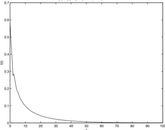
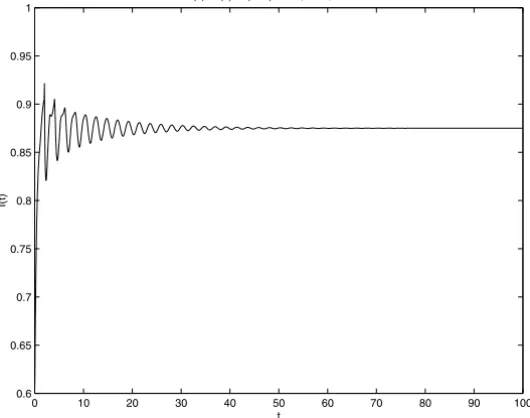
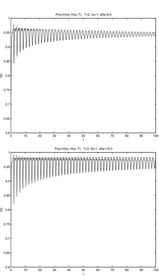
interval[0, t0+T] due to the arbitrary choice of initial data but, as it can be seen, the infection process is self controlled, tending to disappear for increasing tvalues. On the other hand, Fig. 2, 3 and 4 show the more complex situation of typical‘‘fast infective rate cases’’αT >1. In each case, strong (but damped) oscillations would appear for αT large enough. Nevertheless, an equilibrium pointI∞=(αT −1)/αT is attained fort → +∞, characterizing an endemic situation.
0 10 20 30 40 50 60 70 80 90 100
0 0.1 0.2 0.3 0.4 0.5 0.6 0.7
t
I(t)
P(s)=H(s)−H(s−T): T=2, to=1, alfa=0.45
Figure 1 – Density of infected computers as a function of time in aslow infective rate
case. We considerg(t )=I0/T =0.3 fort ∈ [−T −t0,0],α=0.45,t0=1,T =2
andP (t, τ ) = φ (t−τ ), whereφ (ξ )is the characteristic function of [0, T[. Notice that in this case, the infection process affecting the system tends to disappear fortlarge
enough, in agreement with the previous results.
As it was shown in the previous section, the stationary solutionI∞ =0 is an asymptotically stable solution forρT =αT <1. This means that when such a
condition holds, the introduction of a few infected computers into an infective-free population won’t give rise to an epidemic outbreak and also no endemic situations will be developed, i.e., the infection will vanish along the time.
hypothesis included, the present work constitutes a first attempt to explain the virtual virus propagation process in a system of interacting computers and re-veals some features. These result, we hope, could stimulate future researches in such a current problem. At present, we are engaged in the developing of more sophisticated models in order to take into account immunity factors (the exis-tence of vaccines) as well as to include the spatial dependence of the infectious process. Results in this direction will be published elsewhere.
0 10 20 30 40 50 60 70 80 90 100
0.6 0.65 0.7 0.75 0.8 0.85 0.9 0.95 1
t
I(t)
P(s)=H(s)−H(s−T): T=2, to=1, alfa=4.0
Figure 2 – Density of infected computers as a function of time in afast infective rate
case. Hereg(t )=I0/T =0.3 fort ∈ [−T −t0,0],α=4.0,P (t, τ ), t0andT are the
same as in Figure 1. An equilibrium endemic situation (I∞=(αT−1)/αT) is attained
whent → ∞, as can be seen from the figure. This last behavior seems to be a general
one forαT >1, because using different parameters in numerical calculations we have always obtained such a result.
5 Acknowledgments
0 10 20 30 40 50 60 70 80 90 100 0.6
0.65 0.7 0.75 0.8 0.85 0.9 0.95 1
t
I(t)
P(s)=H(s)−H(s−T): T=2, to=1, alfa=9.0
0 10 20 30 40 50 60 70 80 90 100
0.6 0.65 0.7 0.75 0.8 0.85 0.9 0.95 1
t
I(t)
P(s)=H(s)−H(s−T): T=2, t0=1, alfa=15.0
REFERENCES
[1] N.J.T. Bailey,The Mathematical Theory of Infectious Diseases and its Applications, Griffin, London (1975).
[2] C.T.H. Bakes and G.F. Miller,Treatment of Integral Equations by Numerical Methods, Aca-demic Press (1982).
[3] R. Bellmann and K.L. Cooke,Differential-Difference Equations, Math. in Sciences and Engineering, Academic Press (1963).
[4] V. Capasso,Mathematical Structure of Epidemic systems, Springer-Verlag (1993).
[5] J.A. Cochran,The Analysis of Linear Integral Equations, MacGraw-Hill, Meth. Appl. Math., (1972).
[6] K.L. Cooke and J.A. Yorke,Some equations modelling growth processes and gonorrhea epidemics, Mathematical Biosciences,16(1973), pp. 75–101.
[7] R.D. Driver,Ordinary and Delay Differential Equations, Applied Mathematical Sciences, 3(1977), Springer-Verlag.