eve rosouza solution

Solution of Saint Venant's Equation to Study Flood in Rivers,

through Numerical Methods.

Chagas, Patrícia

Department of Environmental and Hydraulics Engineering, Federal University of Ceará

Souza, Raimundo

Department of Environmental and Hydraulics Engineering, Federal University of Ceará

Abstract. The problems of flood wave propagation, in bodies of waters, caused by intense rains or breaking of control structures, represent a great challenge in the mathematical modeling processes. The solution of this problem passes, invariably, for the development of mathematical models that, in their formulations, describe, in the closest it way, the real scenery of the process. On the other hand, the mathematical manipulation of those models implies in the solution of nonlinear differential equations, as it is the case of Saint Venant's Equation, of great application in the studies of rivers, for gradually varied flow. This research uses a discretization, for the equations that governs the propagation of a flood wave, in natural rivers, with the objective of a better understanding of this propagation process. The results have shown that the hydraulic parameters play important game in the propagation of a flood wave.

Keywords: Hydrodynamics Models, Flood Control, Flow in Natural Rivers.

1. Introduction

The study of the flow in open channels is an important topic of the hydraulics and the hydrology subjects. As Brazil is a privileged country in terms of water resources, the necessity of the rational and the sustained use of the rivers becomes an indispensable task. Being like this, the technical and scientific community linked to the theme is seeking, more and more, to supply subsidies inherent to problems related with water resources management.

In this work it intends to study the propagation of a flood wave natural river, originating from torrential rains or of the breaking of a control structure. A wave is defined as a temporary and space variation in the properties and hydraulic characteristics of the flow, just as the change in the flow or in the height of the surface of water (Porto, 2003). This is a physical process of high complexity and it needs for its solution the knowledge of all hydrodynamics of the hydraulic system.

The hydrodynamic model, which is composed by the differential equations of Saint-Venant, allows, in their main analysis, that the study of the hydraulic and hydrologic behavior of this body of water could be made. In that context, through those equations, it is possible to develop a methodology capable to study such variables as flow, velocity and depth in function of the space and

1

temporal coordinates and, finally, to determine every flow structure of the river.

The results obtained in this work allow evaluating how it happens the change in the depth of the surface of water, with the entrance of a wave in the channel, for different roughness coefficient and different bed slope of the channel.

2. Methodology

The basic equations that describe the propagation of a wave in an open channel are the Saint Venant's equations. Those waves can be classified as: dynamic wave, gravitational wave, diffuse wave and cinematic wave, according to the number of elements considered in the model. The dynamic wave, for instance, considers all the terms of the momentum equation. The gravitational wave neglects the bed slope effects, and the friction effect that develops between the water and the walls of the river. In this case, the neglected term is g(S0-Sf). The other terms of the momentum equation are

considered in the modeling. The cinematic wave just considers the effects of the bed slope and the effects of the friction that develops between the water and the walls.

In this work it will be used the dynamic wave. For the development of the mathematical model, some simplifications were made: the flow will be considered one dimensional; the distribution of the pressure in the vertical is hydrostatic one; the water will be considered as incompressible and homogeneous, and the density will be considered constant in the time and in the space. Thus, the model equation could be defined by,

ƒ Continuity Equation

0

= ∂ ∂ + ∂ ∂

t A x Q

(1)

ƒ Momentum Equation

(

)

0 )

( /

0 2

= +

− ∂ ∂ + ∂ ∂ + ∂ ∂

f gAS S

x y gA x

A Q t

Q

(2)

Where x is the longitudinal distance along the channel (m), t is the time (s), A is the cross section area of the flow (m2), y is the surface level of the water in the channel (m), S0 is the slope of bottom of the channel, Sf is the slope of

energy grade line, B is the width of the channel (m), and g is the acceleration of the gravity (m.s-2).

In order to calculate Sf, the Manning formulation will be used. Thus,

2 / 1 3 / 2

1

f S R n

Where V is the mean velocity (m/s), R is the hydraulic radius (m) e n is the roughness coefficient.

Operating algebraically (1), (2) and (3), Keskin (1997), one can find,

0

= + ∂ ∂ + ∂

∂

_α

_β

x Q t

Q

(4)

Where,

⎟ ⎠ ⎞ ⎜

⎝ ⎛ −

− +

=

B R A

Q

A Q B gA A

Q

3 4 3 5 2

2 2

α (5)

and

) (S S₀ gA _f − =

β

In this hydrodynamic model it will certain two dependent variables. The first refers to the cross section area A(x,t), along the channel, for each interval of time. The second one refers to the flow field Q(x,t) along the channel, for the same previous conditions. As the investigation demands the knowledge of two dependent variables, there is the necessity of two differential equations: the equation (1) and the equation (4) will compose the model.

ƒ Initial Conditions:

Q(x,0)=Q0 (7)

A(x,0)=A0 (8)

Where Q0 is the steady state flow of the channel, and the A0 is the cross section area for the steady state conditions.

ƒ Boundary Conditions:

)) 2 sin( . 1 ( ) , 0

( 0

T t a

Q t

Q = +

π

) ( ) , 0

( t h t

Q = , for t>tb (10)

3. Numeric Solution of the Hydrodynamic Model

With respect the numeric solution of the differential equations of the dynamic wave, the explicit discretization formulation will be used and defined through the relationship:

0 ) ( 1 1 1 1 1

1 + =

∆ − + ∆ − + + + + + + m j i j i m j i j i x Q Q t Q Q

β

α

Making an arrangement of the equation (11) it is possible to find:

x t t Q x t Q Q m m j i m j i j i ∆ ∆ + ∆ − ∆ ∆ + = + + + +

α

β

α

1 (12)

Where αm and βm are defined, respectively:

2 1 1 j i j i m + + ₊

=

α

α

α

And 2 1 1 j i j i m + + ₊

=

β

β

β

Finally with the Q calculate for the next time step, it is possible calculate the A(x,t), through:

) (

2 )

( ₁1 1 ₁1 ₁

1 1 1 j i j i j i j i j i j

i q q

Dx Q Q Dx Dt A

A₊+ = ₊ − ₊+ − + + ₊+ + ₊ (15)

4. Results

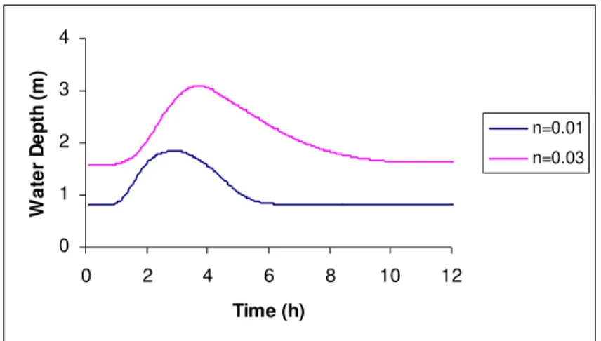
For this work it was developed a hydrodynamic model capable to realize simulations to analyze the behavior of the depth of water, when a flood wave comes into the channel, as function of time. Some considerations were made for the numeric simulation, such as, length of the channel 50.000 meters, width of the channel 50 meters, and sinusoidal function to represent the entrance of a wave in the channel. The discretization in the x direction was made in 50 intervals of 1.000 meters each, totaling a length of 50 km. Regarding discretization of the time, it became divided in 360 intervals, with 150 seconds, totaling a time of 15 hours.

hours, the depth is around 1.8 meters, while for n=0.03 and a time of 4 hours, the pick of the height is close to 3.0 meters.

0 1 2 3 4

0 2 4 6 8 10 12

Time (h)

W

a

te

r D

e

p

th

(m

)

n=0.01

n=0.03

Figure 1 – Comparison among values of water depth for different roughness.

As it can be observed, as bigger is the roughness, the will be the values of the depth of the water in the channel. This happens because the roughness coefficient, n, represents the most important factor in the resistance process concerning with friction effect (Silva et al., 2003).

The Figure 2 shows the comparison among the values of the depth of the water in the channel, in meters, after the entrance of a wave, for different times and with a same value of the roughness n=0.01. As it can be observed, as bigger is the bed slope, the less will be the values of the depth of water in the channel. Thus, for S0=0.0002 and a time of approximately 2:30 hours, the depth is around 1.8 meters, while for S0 =0.0005 and a time of 2:40 hours, the pick of the height is close to 1.4 meters.

0 1 2 3

0 2 4 6 8 10 12

Tim e (h)

W

a

te

r D

e

p

th (m

)

S0=0.0002

S0=0.0005

Figure 2 - Comparison among values of water depth for different bed slope.

5. Conclusions

depth of the channel, with the entrance of a wave, such that it could be able to determine the region with more susceptibility of the occurrence of inundations.

A relevant aspect of this research is in the implementation of a methodology capable to accomplish some simulations, through a computational program, with base in the method of the finite differences, where quite satisfactory results were obtained.

In that way, it was important to verify the reach of the depth of the channel under the influence of a dynamic wave, for different bed slope and roughness coefficient, being verified that the propagation of the flood wave suffers great influence of these parameters.

In the reality, this study allows that subsidies could be obtained, in order to apply in the development of programs of water resources management, especially, in the prevention of inundations. However, it is important to point out that there are still many aspects to research and to implement in the model.

References

Bajracharya, K. Barry, D.A. (1999). Accuracy Criteria for Linearised Diffusion Wave Flood Routing, Journal of Hydrology, v. 195, p. 200-217, Elsevier.

Barry, D.A.; Bajracharya, K. (1995). On the Muskingum-Cunge Flood Routing Method. Environmental International, v. 21, n. 5, p. 485 - 490, Elsevier.

Chalfen, M.; Niemiec, A. (1996). Analytical and Numerical Solution of Sain-Venant Equations. Journal of Hydrology, v. 86, p. 1 – 13.

Chow, V. T., 1988. Applied Hydrology, New York: McGraw-Hill. 572p.

Keskin, M. E.; Agiralioglu, N. A., 1997. Simplified Dynamic Model for Flood Routing in Rectangular Channels. Journal of Hydrology, v. 202, p. 302-314, Elsevier.

Porto, R. de M. P., 2003. Hidráulica Básica. Projeto Reenge. São Carlos: EESC USP, 2ª ed. 540p

Moussa, R.; Bocquillon, C. (1996). Criteria for the choice of Flood-Routing Methods in Natural Channels. Journal of Hydrology, 186, p. 1-30, Elsevier.