Braz. J. Chem. Eng. vol.25 número1

ISSN 0104-6632 Printed in Brazil

www.abeq.org.br/bjche

Vol. 25, No. 01, pp. 183 - 199, January - March, 2008

*To whom correspondence should be addressed

Brazilian Journal

of Chemical

Engineering

PREDICTION OF HIGH-PRESSURE VAPOR

LIQUID EQUILIBRIUM OF SIX BINARY

SYSTEMS, CARBON DIOXIDE WITH SIX

ESTERS, USING AN ARTIFICIAL

NEURAL NETWORK MODEL

C. Si-Moussa

, S. Hanini

, R. Derriche

, M. Bouhedda

and A. Bouzidi

E-mail : simoussa_cherif@yahoo.fr

2_{LBMPT, Université de Médéa, Quartier Ain D’Heb, 26000, Médéa, Algérie.} 3

Centre de Recherche Nucléaire de Birine, Algérie.

(Received: May 4, 2007 ; Accepted : November 5, 2007)

Abstract - Artificial neural networks are applied to high-pressure vapor liquid equilibrium (VLE) related

literature data to develop and validate a model capable of predicting VLE of six CO2-ester binaries (CO2-ethyl

caprate, CO2-ethyl caproate, CO2-ethyl caprylate, CO2-diethyl carbonate, CO2-ethyl butyrate and CO2

-isopropyl acetate). A feed forward, back propagation network is used with one hidden layer. The model has five inputs (two intensive state variables and three pure ester properties) and two outputs (two intensive state variables).The network is systematically trained with 112 data points in the temperature and pressure ranges (308.2-328.2 K), (1.665-9.218 MPa) respectively and is validated with 56 data points in the temperature range (308.2-328.2 K). Different combinations of network architecture and training algorithms are studied. The training and validation strategy is focused on the use of a validation agreement vector, determined from linear regression analysis of the plots of the predicted versus experimental outputs, as an indication of the predictive ability of the neural network model. Statistical analyses of the predictability of the optimised neural network model show excellent agreement with experimental data (a coefficient of correlation equal to 0.9995 and 0.9886, and a root mean square error equal to 0.0595 and 0.00032for the predicted equilibrium pressure and CO2 vapor phase composition respectively). Furthermore, the comparison in terms of average absolute

relative deviation between the predicted results for each binary for the whole temperature range and literature results predicted by some cubic equation of state with various mixing rules and excess Gibbs energy models shows that the artificial neural network model gives far better results.

Keywords: Vapor liquid equilibrium; High pressure; Artificial neural networks; Carbon dioxide; Esters.

INTRODUCTION

The interest in high-pressure phase equilibrium is increasing due to its importance for many chemical processes that are conducted at high pressures in various industries (pharmaceutical, cosmetic, food, petroleum, natural gas etc.) and particularly

ternary systems). Carbon dioxide is the most commonly used supercritical fluid for extraction, and material processing owing to its availability, inertness, non-flammability, non-toxicity, low cost and low critical temperature and pressure. Fundamentals and applications of supercritical fluid technology have been described by McHugh and Krukonis (1994) and Brunner (1994).

Information about the phase behavior of fluid mixtures can be obtained from direct measurement of phase equilibrium data or by the use of equation of state and/or activity coefficient based thermodynamic models. Direct measurement of precise experimental data is often difficult and expensive, while the second method, which includes a large number of equation of states and excess Gibbs free energy models, is tedious and involves a certain amount of empiricism to determine mixture constants, through fitting experimental data and using various arbitrary mixing rules, making difficult the selection of the appropriate model for a particular case.

On the other hand artificial neural networks (ANN), which can be viewed as an universal approximation tool with an inherent ability to extract from experimental data the highly non linear and complex relationships between the variables of the problem handled, have gained broad attention within process engineering as a robust and efficient computational tool. They have been successfully used to solve problems in biochemical and chemical engineering (Baughman and Liu, 1995). Such applications include bioreactor control with unstable parameters (Syu and Tsao, 1993), fault detection and predictive modelling (Ferentinos, 2005), modelling and simulation of a fermentation process, (Hongwen et al., 2005), dynamic modelling, simulation and control of fixed-bed reactor (Shahrokhi and Baghmisheh, 2005), modelling of a continuous fluidized bed dryer (Satish and Setty, 2005), polymerization processes (Fernandes and Lona, 2005), modelling of liquid-liquid extraction column (Chouai et al., 2000), modelling and simulation of CO2-supercritical fluid extraction of black cumin

seed oil (Fullana et al., 1999), and black pepper essential oil (Izadifar and Abdolahi, 2005), and recovery of biological products from fermentation broths (Patnaik, 1999).

As far as thermo physical properties and phase equilibria are concerned, Scalabrin et al. (2002) have used an extended corresponding state NN model to predict residual properties of several pure halocarbons. Chouai et al. (2002) have used an ANN model to estimate the compressibility factor for the

liquid and vapor phase as a function of temperature and pressure for several refrigerants. Laugier and Richon (2003) have used two ANN models, one for the vapor phase and other for the liquid phase, to estimate the compressibility factor and the density of some refrigerants as a function of pressure and temperature. Boozarjomehry et al. (2005) have developed a set of feedforward multilayer neural networks for the prediction of some basic properties of pure substances and petroleum fractions. Khayamian and Esteki (2004) have proposed a wavelet neural network model to predict the solubility of some polycyclic aromatic compounds in supercritical CO2. Tabaraki et al. (2005) have also

used a wavelet neural network to predict the solubility of azo dyes in supercritical CO2 and

Tabaraki et al. (2006) of 25 anthraquinone dyes in supercritical CO2 at different conditions of

temperature and pressure. Havel et al. (2002) have proposed ANN for the evaluation of chemical equilibria.

Applications of ANN for the prediction of VLE have been reported in a number of papers. Petersen et al. (1994) have used ANN to estimate activity coefficient based on group contribution methods. Guimaraes and McGreavy (1995) have reported the use of ANN to estimate VLE in terms of bubble point conditions of the benzene-toluene binary. Sharma et al. (1999), in a paper which emphasizes on the potential advantages of ANN over EOS models for VLE prediction, have reported the use of ANN models which take the equilibrium pressure and temperature as inputs to predict the liquid and vapor phase compositions for low pressure VLE of methane-ethane and ammonia-water binaries. In Urata et al. (2002) work two multilayer perceptrons have been used to estimate VLE of binary systems containing hydrofluoroethers and polar compounds. Ganguly (2003) has used ANN with radial basis functions to predict VLE of binary and ternary systems. Piowtrowski et al. (2003), however, have used a feedforward multilayer neural network to simulate complex VLE in an industrial process of urea synthesis from ammonia and carbon dioxide. Bilgin (2004) has also used feedforward ANN to estimate isobaric VLE in terms of activity coefficients for the methylcyclohexane–toluene and isopropanol–methyl isobutyl ketone systems. More recently, Mohanty (2005) has used multilayer perceptron ANN with one hidden layer to predict VLE in terms of liquid and vapor phase compositions given the equilibrium temperature and pressure for each of the three binary systems (CO2

-Brazilian Journal of Chemical Engineering Vol. 25, No. 01, pp. 183 - 199, January - March, 2008

ethylcaprylate). In another paper Mohanty (2006) has reported the use of ANN to estimate the bubble pressure and the vapor phase composition of the CO2–difluoromethane system. In all the works

reported herein regarding phase equilibrium ANN has been applied to a single binary system at various conditions of equilibrium pressure and temperature.

In this work an attempt was made to estimate high pressure VLE of six CO2-esters binaries using a

single ANN predictive model. Three pure component properties and two intensive state variables have been selected as the NN inputs in order to describe the VLE of the six binaries in one system. The experimental data used for training and validation of the NN are those reported by Hwu et al. (2004) for CO2-ethyl caprate, CO2-ethyl caproate and CO2

-ethyl caprylate systems, and by Cheng and Chen (2005) for CO2-diethyl carbonate, CO2-ethyl butyrate

and CO2-isopropyl acetate systems. As mentioned by

these authors, these systems are of importance for supercritical fluid extraction. Isopropyl acetate, ethyl butyrate and ethyl caprylate are used as perfumes or aroma additives in cosmetic and food industries, whereas diethyl carbonate, ethyl caproate and ethyl caprate are used in organic synthesis, in the production of essential oils and in the production of resin.

NEURAL NETWORK MODELLING

Feedforward Artificial Neural Networks Concept

The idea of artificial neural networks was inspired in the way biological neurons process information. This concept is used to implement software simulations for the massively parallel processes that involve processing elements interconnected in network architecture. Learning in the human brain occurs in a network of neurons that are interconnected by axons, synapse and dendrites. A variable synaptic resistance affects the flow of information between two biological neurons. The artificial neuron receives inputs that are analogous to the electrochemical impulses that the dendrites of biological neurons receive from other neurons. Therefore, ANN can be viewed as a network of neurons which are processing elements and weighted connections. The connections and weights are analogous to axons and synapses in the human brain respectively. The ANN, simulating human brain analytical function, has an intrinsic ability to learn and recognize highly non-linear and complex relationships by experience.

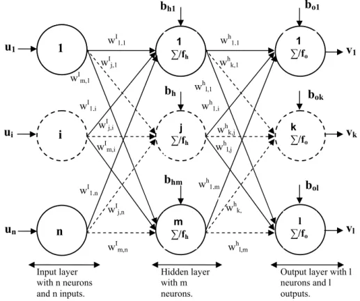
The artificial neurons are arranged in layers (Fig. 1) wherein the input layer receives inputs (ui) from

the real world and each succeeding layer receives weighted outputs (wij.ui) from the preceding layer as

its input resulting therefore a feedforward ANN, in which each input is fed forward to its succeeding layer where it is treated. The outputs of the last layer constitute the outputs to the real world.

In such a feedforward ANN a neuron in a hidden or an output layer has two tasks:

ƒ It sums the weighted inputs from several connections plus a bias value and then applies a transfer function to the sum as given by (for neuron j of the hidden layer):

n I

j h ji i hj i 1

z f w u b ; j 1, 2, ... , m

=

 

= _ + _ =



∑

ƒ It propagates the resulting value through outgoing connections to the neurons of the succeeding layer where it undergoes the same process as given by (for instance outputs z of the hidden layer fed to neuron _j

k of the output layer gives the outputv ): _k

m h

k O kj j ok

j 1

v f w z b ;

k 1, 2, ... , l

=     = +     =

∑

Combining equations 1 and 2 the relation between the output v and the inputs _k u of the NN is obtained: _i

m n

h I

k O kj h ji i hj ok

j 1 i 1

v f w f w u b b ;

k 1, 2, ... , l

= =       = _ + _+  _{ }    =

∑

∑

The output is computed by means of a transfer function, also called activation function. It is desirable that the activation function has a sort of step behavior. Furthermore, because continuity and derivability at all points are required features of the current optimization algorithms, typical activation functions which fulfill these requirements are:

ƒ Hyperbolic tangent sigmoid transfer function:

a a a a e e f (a) e e − − − =

ƒ Logarithmic sigmoid transfer function:

a

1 f (a)

1 e−

=

+ (5)

ƒ Pure linear transfer function:

f (a)=a (6)

The number of neurons in the input and output layers is determined by the number of independent and dependent variables respectively. The user defines the number of hidden layers and the number of neurons in each hidden layer. Model development is achieved by a process of training in which a set of

experimental data of the independent variables are presented to the input layer of the network. The outputs from the output layer comprise a prediction of the dependant variables of the model. The network learns the relationships between the independent and dependent variables by iterative comparison of the predicted outputs and experimental outputs and subsequent adjustment of the weight matrix and bias vector of each layer by a back propagation training algorithm. Hence, the network develops a NN model capable of predicting with acceptable accuracy the output variables lying within the model space defined by the training set. Consequently, the objective of ANN modelling is to minimize the prediction errors of validation data presented to the network after completion of the training step.

Figure 1: Three-layer feedforward neural network.

Selection of a Neural Network Model

Although there is continuing debate on model selection strategies, it is clear that the successful application of ANN in modelling engineering problems is highly affected by four major factors: 1. Network type (recurrent networks, feedforward backpropagation, wavelet neural network, radial basis functions, etc.),

2. Network structure (number of hidden layers, number of neurons per hidden layer),

3. Activation functions, 4. Training algorithms.

It is well established that the variation of the number of neurons of the hidden layer(s) has a significant effect on the predictive ability of the network. For Plumb et al. (2005) the most common way of optimizing the performance of ANN is by

Output layer with l neurons and l outputs. Hidden layer

with m neurons. Input layer

with n neurons and n inputs.

v

whk,j

b

b

b

∑/F 1 ∑/fh

j ∑/fh

m ∑/fh

wI1,1

wIj,1

wIm,1

wI1,i

wIj,i

wIm,i

wI1,n

wIj,n

wIm,n

1

i

n

wh1,1

whk,1

whl,1

wh1,i

whl,j

wh1,m

whk,

whl,m

1 ∑/fo

k ∑/fo

l ∑/fo

b

b

b

v

v

u

u

Brazilian Journal of Chemical Engineering Vol. 25, No. 01, pp. 183 - 199, January - March, 2008

varying the numbers of neurons in the hidden layer(s) and selecting the architecture with the highest predictive ability. According to Swingler (1996) a heuristic rule suggests that for multilayer NN with one hidden layer the hidden layer will never require neurons more than twice the inputs. However, Curry and Morgan (2006), who have discussed relating difficulties in the selection of a neural network structure, state that heuristic rules have little to offer and such rules, suggesting that the number of hidden neurons should be directly related to the number of inputs and outputs, have only historical interest, being popular immediately after the path finding work of Rumelhart et al. (1986). With regard to methods of choosing the number of hidden layers and hidden neurons in the design of a NN model, Curry and Morgan (2006) findings show that neither heuristics nor statistical concepts can be used conclusively. They concluded that the most simple, and probably still the most popular sensible, strategy (practitioner’s strategy as they labeled it) is to focus directly on minimizing the root mean square error. The obvious difficulty for this strategy is the excessive computational burden brought about by the time consuming process of experimenting different models: the cause is ‘combinatorial explosion’ in the number of different NN models which need to be run. Henrique et al. (2000) presented a procedure, for model structure determination in feedforward networks, which is based on network pruning using orthogonal least-squares techniques to determine insignificant or redundant synaptic weights, biases, hidden neurons and network inputs.

As far as training algorithms are concerned, the following classes of algorithms, which are implemented in MATLAB® neural network toolbox, are the most commonly used algorithms: Levenberg-Marquardt backpropagation (Hagan and Menhaj, 1994); Bayesian regularization backpropagation (MacKay, 1992; Foresee and Hagan, 1997); conjugate gradient backpropagation (Moller, 1993; Powell, 1977); gradient descent backpropagation (Hagan et al., 1996); quasi-Newton (Battiti , 1992).

A significant problem with ANN training is the tendency to over-train resulting in a lack of ability to predict, accurately, data excluded from the training set. To overcome this, test data set may be presented to the network during training in such a way that training will terminate at the point where the error of the test set predictions begins to diverge. This method is known as “stopped training” (Bourquin et

al., 1997) or “attenuated training” (Plumb et al., 2002; Plumb et al., 2005). Attenuated training is generally applicable to gradient descent, conjugate gradient and quasi-Newton training algorithms. Bayesian regularization training algorithm uses a modified performance function designed to minimize over-training by smoothing the error surface of the training set. Plumb et al. (2005) have compared these classes of algorithms and three different NN packages when applied to problems in the pharmaceutical industry. Amongst their conclusions, is that MATLAB/Bayesian regularization models train more successfully than MATLAB models using attenuated training. They too have proposed the trail and error strategy (practitioner’s strategy) for the selection of the best NN structure and training algorithms focusing on the goodness of fit, R2, determined for validation plots of the predicted versus observed data, as a measure of the predictive ability of the model.

VLE MODELLING WITH NEURAL NETWORK

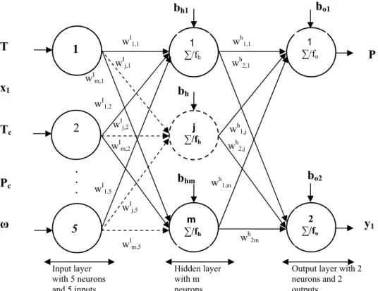
In order to describe the phase behavior of the six CO2(1)-ester(2) binaries by one ANN model a total

of seven variables have been selected in this work: four intensive state variables (equilibrium temperature, equilibrium pressure and equilibrium CO2 mole fractions in the liquid and vapor phases)

and three pure component properties of the ester (critical temperature, critical pressure and acentric factor). The choice of the input and output variables was based on the phase rule, practical considerations (bubble or dew point computation) and the need to describe the six binaries by only one ANN model. Therefore, the equilibrium temperature, the CO2

mole fraction in the liquid phase together with the pure component properties of the esters have been selected as input variables and the remaining as output variables (Fig.2).

The experimental data reported by, Hwu et al. (2004) for CO2-ethyl caprate, CO2-ethyl caproate and

CO2-ethyl caprylate systems and Cheng and Chen

(2005) for CO2-diethyl carbonate, CO2-ethyl butyrate

and CO2-isopropyl acetate systems, have been used

Figure 2: Three-layer VLE feedforward neural network for the prediction of bubble pressure and vapor phase composition.

Table 1: Pure component properties used in this work

Component Tc (K) Pc (MPa) ω Reference

Ethyl caprate 680.82 1.788 0.742 (Hwu et al., 2004)

Ethyl caproate 611.62 2.548 0.555 (Hwu et al., 2004)

Ethyl caprylate 648.64 2.118 0.653 (Hwu et al., 2004)

Diethyl carbonate 576.00 3.390 0.485 (Cheng and Chen, 2005)

Ethyl butyrate 566.00 3.060 0.463 (Cheng and Chen, 2005)

Isopropyl acetate 538.00 3.580 0.355 (Cheng and Chen, 2005)

Table 2: Source and range of data used for training and validation of the artificial neural network model

System T (K) P (MPa) x1 y1 N Reference

308.2 1.665-7.109 0.2580-0.8454 0.9998 9 (Hwu et al., 2004) 318.2 1.699-7.891 0.2297-0.7775 0.9996-0.9998 10 (Hwu et al., 2004) CO2-ethyl caprate

328.2 1.699-9.218 0.2068-0.7780 0.9992-0.9998 11 (Hwu et al., 2004) 308.2 1.699-6.462 0.2823-0.8480 0.9990-0.9994 8 (Hwu et al., 2004) 318.2 1.699-7.823 0.2301-0.8541 0.9976-0.9992 10 (Hwu et al., 2004) CO2-ethyl caproate

328.2 1.733-9.218 0.2090-0.8463 0.9963-0.9987 12 (Hwu et al., 2004) 308.2 1.75-7.177 0.2786-0.8904 0.9995-0.9997 9 (Hwu et al., 2004) 318.2 1.699-7.823 0.2407-0.8063 0.9992-0.9997 10 (Hwu et al., 2004) CO2-ethyl caprylate

328.2 1.699-9.218 0.2088-0.8156 0.9985-0.9996 12 (Hwu et al., 2004) 308.45 4.72-7.14 0.500-0.892 0.9947-0.9973 9 (Cheng and Chen, 2005) 313.45 4.50-7.69 0.450-0.840 0.9950-0.9983 9 (Cheng and Chen, 2005) CO2-diethyl carbonate

318.55 4.30-8.20 0.400-0.780 0.9933-0.9977 10 (Cheng and Chen, 2005) 308.45 4.80-6.80 0.480-0.810 0.9940-0.9974 7 (Cheng and Chen, 2005) 313.45 4.60-7.90 0.430-0.820 0.9950-0.9983 8 (Cheng and Chen, 2005) CO2-ethyl butyrate

318.55 4.55-8.90 0.395-0.860 0.9940-0.9985 8 (Cheng and Chen, 2005) 308.45 3.30-6.40 0.462-0.880 0.9933-0.9974 8 (Cheng and Chen, 2005) 313.45 3.08-7.16 0.400-0.897 0.9930-0.9973 8 (Cheng and Chen, 2005) CO2-isopropyl acetate

318.55 3.06-7.80 0.360-0.899 0.9929-0.9967 10 (Cheng and Chen, 2005) The six binaries 308.2-328.2 1.665-9.218 0.2068-0.899 0.9929-0.9998 168

Output layer with 2 neurons and 2 outputs. Hidden layer

with m neurons. Input layer

with 5 neurons and 5 inputs.

y1 wh1,j

bhm bh bh1

∑/F

1

∑/fh

j

∑/fh

m

∑/fh wI1,1

wIj,1

wIm,1

wI1,2

wIj,2

wIm,2

wI1,5

wIj,5

wIm,5

1

5

wh1,1

wh2,1

wh2,j

wh1,m

wh2m

1

∑/fo

2 ∑/fo

bo2 bo1

P

2

. . . T

x1

Tc

Pc

Brazilian Journal of Chemical Engineering Vol. 25, No. 01, pp. 183 - 199, January - March, 2008

The application of ANN modelling of VLE of the six CO2-ester binaries was performed using

MATLAB® (version 6.1) and the strategy proposed by Plumb et al. (2005) as follows:

1. The experimental data should be divided into a training set, a test set (when attenuated training is adopted) and a validation set. Each data set should be well distributed throughout the model space.

2. Initially, the model should be trained using the default training algorithm and network architecture. The parameters of the equation of the best fit (the slope and the y intercept of the linear regression) or the goodness of fit (correlation coefficient, R2) are determined for validation plots of the predicted versus the experimental properties of the validation data set. These parameters are used as a measure of the predictive ability of the model. Where the

agreement vector values approach the ideal, i.e. [α=1 (slope), β=0 (y intercept), R2=1], little improvement in predictive ability is to be expected. The ANN model with the best agreement vector is retained and the procedure is stopped.

3. Where the values of the parameters of the agreement vector vary greatly from the ideal and the model is poorly predictive, modification of the number of hidden layer neurons is then considered.

4. If model performance remains unsatisfactory a systematic investigation of the effect of varying both the training algorithm and network architecture is required.

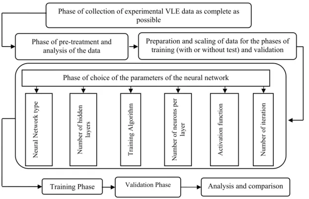
Based on this global strategy, details of the different phases of the procedure followed in this work are depicted in Figure 3.

Figure 3: Procedure for vapor liquid equilibrium neural network modelling

All the input and output data were scaled so as to have a normal distribution with zero mean and unit standard deviation using the following scaling equation:

Scaled value = (Actual value-µ)/ σ (7)

Where µ and σ: are the mean and standard deviations of the actual data respectively. The values of µ and σ for the input and output data, referred to in Table 1 and Table 2, are listed in Table 3. MATLAB neural network toolbox contains various pre and post data

processing methods. When using the above scaling method, scaling and de-scaling are carried out by prestd and poststd MATLAB functions respectively. In order to have data sets well distributed throughout the model space, the data points referred to in Table 2 were sorted in increasing order of the equilibrium temperature and CO2 mole fraction in the liquid

phase, then two records have been used for training and the third for validation which resulted in a two third (112 data points) one third (56 data points) partitions for training and validation respectively. Whenever attenuated training was used, the initial

Phase of collection of experimental VLE data as complete as possible

Phase of pre-treatment and analysis of the data

Phase of choice of the parameters of the neural network

Neural N

etwork

type

Number of

hidd

en

la

y

ers

Number of

neur

ons per

la

y

er

Train

ing Algorithm

Activa

tion fun

cti

on

Number of

it

erat

ion

Training Phase Validation Phase Analysis and comparison

training set (112 data points) was divided, in the same way, into a training set (75 data points) and a test set (37 data points).

The above strategy was implemented in a MATLAB program for ANN modelling of the VLE of six CO2(1)-ester(2) as described in Figure 2.

Initially, the program starts with the default feedforward backpropagation NN type (newff MATLAB function), the Levenberg-Marquardt backpropagation training algorithm (trainlm MATLAB training function) and one hidden layer. Once the topology is specified the starting and ending number(s) of neurons in the hidden layer(s) have to be specified. The number of neurons in a hidden layer is then modified by adding neurons one at a time. The procedure begins with the logarithmic sigmoid activation function and then

the hyperbolic tangent sigmoid activation function for the hidden layers and the linear activation function for the output layer. The results of different runs of the program show, as pointed out by Plumb et al. (2005), that the Bayesian regularization backpropagation, using Levenberg-Marquardt optimization (BRBP) models, train more successfully than models using attenuated training. Table 4 shows the structure of the optimized NN model. The weight matrices and bias vectors of the optimized NN model are listed in Table 5, where wI is the input-hidden layer connection weight matrix (20 rows x 5 columns), wh is the hidden layer-output connection weight matrix (2 rows x 20 columns), bh is the hidden neurons bias column vector (20 rows) and bo is the output neurons bias column vector (2 rows).

Table 3: Mean and standard deviation constants used for scaling and de-scaling of the data

T (K) x1 Tc (K) Pc (MPa) ω y1 P (MPa)

µ 316.69 0.59353 607.23 2.7031 0.55126 0.99776 5.3557

σ 7.1613 0.17636 49.381 0.6593 0.12754 0.0020015 1.8574

Table 4: Structure of the optimized ANN model

Input layer Hidden layer Output layer

Type of network

Training

Algorithm No. of

neurons

No. of neurons

Activation function

No. of neurons

Activation function

FFBP NN (newff

MATLAB function)

BRBP using Levenberg-Marquardt optimization. (trainbr MATLAB function)

5 20 Logarithmic sigmoid (logsig

MATLAB function)

2

Linear (purelin

MATLAB function)

Table 5: Weights and bias of the optimized ANN model

Input-Hidden layer connections Hidden layer -Output connections

Weights Bias Weights Bias

I j1

w wI_j2 wI_j3 wI_j4 wI_j5 b_hj w_1jh wh_{2 j} b_Ok

0.5018 1.8396 -0.2878 0.7773 -0.5557 -4.0379 -3.0596 -2.2766 1.2944 -2.4035 -0.4145 -2.7469 2.4579 0.5453 5.0129 -0.2689

2.7849 0.2721 -0.5708 -0.6904 1.04 0.2338 -3.3433 0.0914

3.7254 0.765 1.6882 1.4707 -0.1082 1.3218 2.8282 -0.0482 -0.2008 0.6928 -2.7705 1.6505 4.4493 -0.2483 -0.0787 3.4188 -1.3349 -1.5401 0.3496 -1.7726 -1.3159 0.1811 0.2522 -0.9687 -1.6961 2.3225 -1.5449 -0.179 4.7975 -0.697 -6.1496 -0.0411

-1.4897 2.4103 3.3415 -0.6834 -1.2443 -0.2042 4.1022 -0.0367

1.8366 6.5943 -0.5975 -0.4448 3.6849 -2.0103 -4.0838 -0.321

-0.1519 0.6817 2.59 -1.0644 0.8603 3.0209 1.9837 -0.7544

2.2935 -2.9871 -3.3568 -1.0277 -3.8443 2.5532 -1.982 -0.0169

-1.9632 -6.9732 -5.1545 -1.32 0.3744 1.9491 -3.828 -0.2611

1.2156 1.9491 -0.0813 1.484 0.7212 -3.4609 -2.1424 2.2304

-0.0732 2.6572 -2.2517 0.9033 0.796 -1.9423 5.6451 -0.3315

0.8129 -0.6547 1.1751 1.8836 -0.0552 -1.4889 -1.3644 -1.217

-2.7793 3.2036 -4.6268 0.0892 -2.2334 -1.4956 3.2525 -0.2122

1.8867 -1.3888 1.1105 -0.8511 -0.1643 -3.1546 1.4405 -0.0771

0.6958 0.4805 -1.2333 -3.0723 -1.67 0.6673 -0.9142 2.0869

0.6806 -2.6749 -0.6764 0.3451 -0.4292 1.8682 -0.9104 0.0746 -0.521 3.0896 2.7228 2.1312 -3.1468 -2.9222 -3.7429 0.0124

Brazilian Journal of Chemical Engineering Vol. 25, No. 01, pp. 183 - 199, January - March, 2008

RESULTS AND DISCUSSION

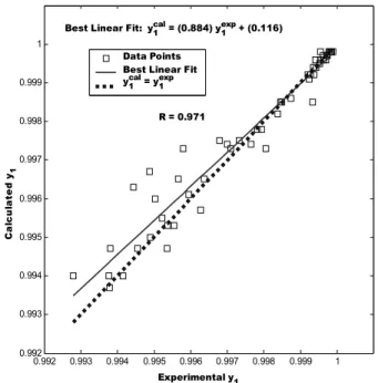
The predictive ability assessment requires evaluation of data records excluded from the training set. Accordingly, the validation agreement vector and the validation agreement plot of the predicted versus the experimental outputs for the validation data set were used to evaluate the predictive ability of the NN model. The plot and the parameters of the linear regression are, straightforwardly, obtained using

postreg MATLAB function. Figure 4 shows the

validation agreement plot for the equilibrium pressure with an agreement vector approaching the ideal, [α, β, R2] = [1.01, -0.0235, 0.999]. Figure 5 shows the same plot for CO2 mole fraction in the vapor phase with an

agreement vector equal to [0.884, 0.115, 0.971]. Table 6 shows the validation agreement vector calculated per binary for the training and validation data sets. It shows that the least favorable regression parameters are those obtained for the prediction of the vapor phase composition of the CO2 (1)-ethyl

caprylate (2) system.

1 2 3 4 5 6 7 8 9 10

1 2 3 4 5 6 7 8 9 10

Experimental equilibrium pressure (MPa)

C

a

lc

u

la

te

d

e

q

u

ilib

ri

u

m

p

re

s

s

u

re

(M

P

a

)

Best Linear Fit: Pcal = (1.01) Pexp+ (-0.0235)

R = 0.999 Data Points Best Linear Fit Pcal = Pexp

Figure 4: Validation agreement plot of the most predictive model of the equilibrium pressure

0.992 0.993 0.994 0.995 0.996 0.997 0.998 0.999 1 0.992

0.993 0.994 0.995 0.996 0.997 0.998 0.999 1

Experimental y₁

C

al

c

ul

a

ted y

1

Best Linear Fit: y₁cal = (0.884) y₁exp + (0.116)

R = 0.971 Data Points Best Linear Fit y₁cal = y₁exp

Table 6: Validation agreement vector [α (slope), β (y intercept), R2 (correlation coefficient] of the NN outputs per binary for the training and validation phases

CO2 (1) – ethyl caprate(2)

CO2 (1) – ethyl caproate(2)

CO2 (1) – ethyl caprylate (2)

CO2 (1) – iethyl carbonate(2)

CO2 (1) – ethyl butyrate(2)

CO2 (1) -isopropyl acetate(2)

The six binaries N 30 30 31 28 23 26 168

P 1.0057 1.0103 1.0008 1.0012 0.9996 1.0002 1.0025

α _y

1 0.8756 0.7403 1.4475 0.9571 0.8727 0.9904 0.9575

P -0.0231 -0.0346 0.0066 -0.0048 -0.0170 0.0068 -0.0088

β _y

1 0.1244 0.2594 -0.4474 0.0429 0.1269 0.0097 0.0425

P 0.9999 0.9993 0.9998 0.9985 0.9979 0.9993 0.9995 R2

y1 0.8914 0.9584 0.7303 0.9801 0.9506 0.9383 0.9886

Table 7 represents the commonly used deviations calculated for the two predicted outputs of the NN model (P: equilibrium pressure, y1: CO2 mole

fraction in the vapor phase) for the whole data set: Average Absolute Relative Deviation:

N exp cal

exp

i 1 _i

100 P P

AARDP(%)

N _{= P}

−

=

∑

exp cal N

1 1

1 _exp

i 1 1 _i

y y

100 AARDy (%)

N _{= y}

−

=

∑

Average Absolute Deviation:

N

exp cal

i 1 i

1

AADP(%) P P

N ₌

=

∑

N

exp cal

1 1 1

i 1 i

1

AADy (%) y y

N ₌

=

∑

Root Mean Square Error (square root of the average sum of squares):

N

exp cal 2 i i i 1 1

RMSEP (P P )

N ₌

=

∑

(

)

N ₂

exp cal

1 1 1 _i

i 1 1

RMSEy y y

N ₌

=

∑

The maximum of the Absolute Relative Deviation is equal to 4.95% and 0.19% for P and y1

respectively. Similarly, the maximum of the Absolute Deviation is equal to 0.42 MPa and 0.0019 for P and y1 respectively.

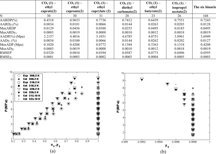
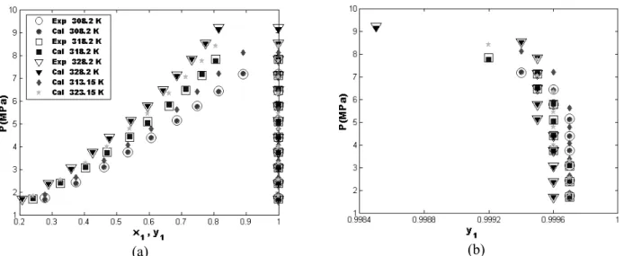
Figures 6-11 show the bubble pressure and dew pressure curves for the six CO2(1)-ester(2) binaries.

They include a comparison between experimental data and NN predicted results at three temperatures and two test temperatures inside the range of experimental data in order to show the interpolating ability of the ANN model. For the three experimental temperatures (shown as circles, squares and downward-triangles), the figures show excellent agreement between experimental literature data (shown as white face markers) and the NN predicted results (shown as dark face markers). For the two test temperatures (shown as dark face pentagrams and diamonds) the predicted bubble and dew curves follow exactly the trend of the experimental data of adjacent temperatures which suggests a good predictive ability of the NN model for temperatures within the range of temperature for which the model has been designed.

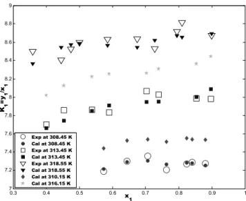
The predictions of CO2 mole fraction in the vapor

phase for the three temperatures for which experimental data are available and the two test temperatures are shown (Fig. 12) in term of the plots of the K-value of CO2 versus the CO2 mole fraction

in the liquid phase for the sample case (CO2 (1)-

Brazilian Journal of Chemical Engineering Vol. 25, No. 01, pp. 183 - 199, January - March, 2008

Table 7: Statistical analyses of the error of the predicted results for the training and validation phases

CO2 (1) – ethyl caprate(2)

CO2 (1) – ethyl caproate(2)

CO2 (1) – ethyl caprylate (2)

CO2 (1) - diethyl carbonate(2)

CO2 (1) – ethyl butyrate(2)

CO2 (1) -isopropyl acetate(2)

The six binaries

N 30 30 31 28 23 26 168

AARDP(%) 0.4518 0.9653 0.7736 0.7412 0.6439 0.7551 0.7243 AARDy1(%) 0.0034 0.0101 0.0066 0.0144 0.0263 0.0203 0.0128

MaxARDP 0.0129 0.0456 0.0388 0.0255 0.0495 0.0185 0.0495 MaxARDy1 0.0003 0.0019 0.0008 0.0010 0.0012 0.0018 0.0019

AADP(%) (Mpa) 2.2157 4.4016 3.1031 4.6785 4.0751 3.8961 3.6949 AADy1(%) 0.0034 0.0100 0.0066 0.0144 0.0262 0.0202 0.0127

MaxADP (Mpa) 0.1020 0.4208 0.0772 0.1384 0.3363 0.1318 0.4208 MaxADy1 0.0003 0.0019 0.0008 0.0010 0.0012 0.0018 0.0019

RMSEP 0.0320 0.0854 0.0394 0.0587 0.0773 0.0496 0.0595

RMSEy1 0.0001 0.0003 0.0002 0.0003 0.0004 0.0005 0.0003

(a) _(b)

Figure 6: P-x-y curves for the CO2(1)-ethyl caprate(2) system at different temperatures : (a):

P-x-y curves; (b) zoom of the dew curves (Exp: (Hwu et al., 2004), Cal: this work);

(a) (b)

Figure 7: P-x-y curves for the CO2 (1)-ethyl caproate (2) system at different temperatures: (a):

(a) (b)

Figure 8: P-x-y curves for the CO2 (1)-ethyl caprylate (2) system at different temperatures: (a): P-x-y curves;

(b): zoom of the dew curves (Exp: (Hwu et al., 2004), Cal: this work)

(a) (b)

Figure 9: P-x-y curves for the CO2 (1)-diethyl carbonate (2) system at different temperatures: (a): P-x-y curves;

(b): zoom of the dew curves (Exp: (Cheng and Chen, 2005), Cal: this work)

(a) (b)

Figure 10: P-x-y curves for the CO2 (1)- ethyl butyrate (2) system at different temperatures: (a): P-x-y curves;

Brazilian Journal of Chemical Engineering Vol. 25, No. 01, pp. 183 - 199, January - March, 2008

(a) (b)

Figure 11: P-x-y curves for the CO2 (1)- isopropyl acetate (2) system at different temperatures: (a): P-x-y

curves; (b): zoom of the dew curves (Exp: (Cheng and Chen, 2005), Cal: this work)

0.3 0.4 0.5 0.6 0.7 0.8 0.9 1

7 7.2 7.4 7.6 7.8 8 8.2 8.4 8.6 8.8 9

x

1

K1

=y

1

/x

1

Exp at 308.45 K Cal at 308.45 K Exp at 313.45 K Cal at 313.45 K Exp at 318.55 K Cal at 318.55 K Cal at 310.15 K Cal at 316.15 K

Figure 12: K-value of CO2 versus CO2 mole fraction in the liquid phase for the CO2(1)- isopropyl acetate(2)

system at different temperatures (Exp: (Cheng and Chen, 2005), Cal: this work)

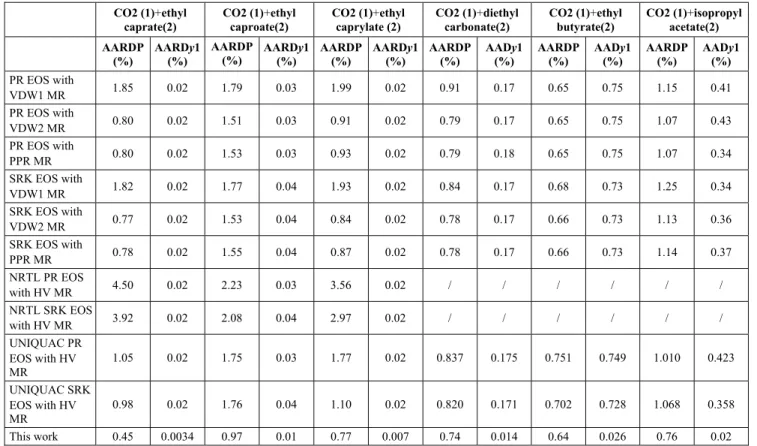
In order to establish the developed NN model as plausible alternative to some cubic EOS and GE models for VLE data prediction of the CO2-ester

systems studied herein, the results obtained by the ANN model were compared to the experimental data reported by Hwu et al. (2004) for CO2-ethyl

caprate, CO2-ethyl caproate and CO2-ethyl

caprylate systems, and by Cheng and Chen (2005) for CO2-diethyl carbonate, CO2-ethyl butyrate and

CO2-isopropyl acetate systems. They relate the

predicted results for each binary for the entire temperature range using Peng-Robinson (PR) and

Soave-Redlick-Kwong (SRK) EOS, with the one and two parameters Van der Waals (VDW1 and VDW2) mixing rules (MR), and the Panagiotopoulos-Reid (PPR) mixing rules and also those predicted using NRTL and UNIQUAC combined with PR and SRK EOS with Huron-Vidal (HV) mixing rules. The results of the comparison are shown in Table 8. It shows that the % deviations of the NN model predicted bubble pressure and CO2 mole fraction in the vapor phase

Table 8: Comparison between the literature results ((Hwu et al., 2004); (Cheng and Chen, 2005)) predicted by some EOS and GE models and the present work for the entire data set

CO2 (1)+ethyl caprate(2)

CO2 (1)+ethyl caproate(2)

CO2 (1)+ethyl caprylate (2)

CO2 (1)+diethyl carbonate(2)

CO2 (1)+ethyl butyrate(2)

CO2 (1)+isopropyl acetate(2) AARDP

(%)

AARDy1 (%)

AARDP (%)

AARDy1 (%)

AARDP (%)

AARDy1 (%)

AARDP (%)

AADy1 (%)

AARDP (%)

AADy1 (%)

AARDP (%)

AADy1 (%) PR EOS with

VDW1 MR 1.85 0.02 1.79 0.03 1.99 0.02 0.91 0.17 0.65 0.75 1.15 0.41 PR EOS with

VDW2 MR 0.80 0.02 1.51 0.03 0.91 0.02 0.79 0.17 0.65 0.75 1.07 0.43 PR EOS with

PPR MR 0.80 0.02 1.53 0.03 0.93 0.02 0.79 0.18 0.65 0.75 1.07 0.34 SRK EOS with

VDW1 MR 1.82 0.02 1.77 0.04 1.93 0.02 0.84 0.17 0.68 0.73 1.25 0.34 SRK EOS with

VDW2 MR 0.77 0.02 1.53 0.04 0.84 0.02 0.78 0.17 0.66 0.73 1.13 0.36 SRK EOS with

PPR MR 0.78 0.02 1.55 0.04 0.87 0.02 0.78 0.17 0.66 0.73 1.14 0.37 NRTL PR EOS

with HV MR 4.50 0.02 2.23 0.03 3.56 0.02 / / / / / / NRTL SRK EOS

with HV MR 3.92 0.02 2.08 0.04 2.97 0.02 / / / / / / UNIQUAC PR

EOS with HV MR

1.05 0.02 1.75 0.03 1.77 0.02 0.837 0.175 0.751 0.749 1.010 0.423

UNIQUAC SRK EOS with HV MR

0.98 0.02 1.76 0.04 1.10 0.02 0.820 0.171 0.702 0.728 1.068 0.358

This work 0.45 0.0034 0.97 0.01 0.77 0.007 0.74 0.014 0.64 0.026 0.76 0.02

CONCLUSIONS

A feed forward artificial neural network model has been used to predict the bubble pressure and the vapor phase composition of six CO2-ester binaries

(CO2-ethyl caprate, CO2-ethyl caproate, CO2-ethyl

caprylate, CO2-diethyl carbonate, CO2-ethyl butyrate

and CO2-isopropyl acetate) given the temperature,

the mole fraction of CO2 in the liquid phase and the

critical temperature, the critical pressure and the acentric factor of the ester, in contrast to previous works where ANN have been used to model only one binary. The optimized NN consisted of five neurons in the input layer, 20 neurons in the hidden layer and two neurons in the output layer. This was obtained by applying a strategy based on assessing the parameters of the best fit of the validation agreement plots (slope and y intercept of the equation of the best fit and the correlation coefficient R2) for the validation data set as a measure of the predictive ability of the model. The statistical analysis shows that the model was able to yield quite satisfactorily estimates. Furthermore, the deviations in the prediction of both the bubble pressure and the CO2 mole fraction in the vapor phase are lower than

those obtained by PR and SRK EOS with Van der Waals type mixing rules and those obtained by NRTL and UNIQUAC models. Therefore, the ANN model can be reliably used to estimate the equilibrium pressure and the vapor phase compositions of the CO2

-ester binaries within the ranges of temperature considered in this work. This study also shows that ANN models could be developed for high pressure phase equilibrium for a family of CO2 binaries,

provided reliable experimental data are available, to be used in supercritical fluid processes. Hence, at least for a non expert in selecting appropriate EOS for the application in hand, alternatives to EOS and activity coefficient models are offered to be used in a more reliably and less cumbersome way, in process simulators and processes involving real time process control.

NOMENCLATURE

AAD Average Absolute

Deviation

(-)

AARD Average Absolute Relative Deviation

Brazilian Journal of Chemical Engineering Vol. 25, No. 01, pp. 183 - 199, January - March, 2008

ANN Artificial Neural Networks

(-)

b bias (-)

BRBP Bayesian Regularization Back Propagation

(-)

EOS Equation Of State (-)

f activation function (-)

FFBP Feed Forward Back Propagation

(-)

HV Huron Vidal (-)

K K-value (-)

MaxAAD maximum of the Average Absolute Deviation

(-)

MaxAARD maximum of the Average Absolute Relative Deviation

(-)

MR Mixing Rules (-)

N number of data points (-)

NN Neural Networks (-)

P equilibrium pressure MPa

Pc critical pressure MPa

PPR Panagiotopoulos Reid (-)

PR Peng Robinson (-)

Psat vapor pressure (-)

RMSE Root Mean Square Error (-) R2 correlation coefficient (-)

SRK Soave Redlich Kwong (-)

T equilibrium temperature K

Tc critical temperature K

u neural network input vector

(-)

v neural network output vector

(-)

VDW Van der Waals (-)

w weights (-)

x liquid phase mole fraction (-) y vapor phase mole fraction (-) z hidden layer output vector (-)

Greek Letters

µ mean (-)

α slope of the linear regression equation

(-)

β y intercept of the linear regression equation

(-)

σ standard deviation (-)

ω acentric factor (-)

Subscripts

1 component 1 (-)

2 component 2 (-)

h hidden layer (-)

i component i (-)

ij connection between jth input neuron and ith output neuron.

(-)

o output layer (-)

Superscripts

cal calculated exp experimental

h hidden layer

I input layer

REFERENCES

Battiti, R., First- and second-order methods for learning between steepest descent and Newton’s method, Neural Comput., 4, 141 (1992).

Baughman, D.R. and Liu, Y.A., Neural Networks in Bio-Processing and Chemical Engineering, Academic Press, New York (1995).

Bilgin, M., Isobaric vapour-liquid equilibrium calculations of binary systems using neural network, J. Serb. Chem. Soc., 69, 669 (2004). Boozarjomehry, R.B., Abdolahi, F. and Moosavian,

M.A., Characterization of basic properties for pure substances and petroleum fractions by neural network, Fluid Phase Equilib., 231, 188 (2005). Bourquin, J., Schmidli, H . and van Hoogvest, P.,

Leuenberger, H., Basic concept of artificial neural networks (ANN) modelling in the application of pharmaceutical development, Pharm. Dev. Technol. 2, 95 (1997).

Brunner, G., Gas Extraction, Steinkopff-Verlag, Darmstadt (1994).

Cheng, C.-H. and Chen, Y.-P., Vapor-liquid equilibrium of carbon dioxide with isopropyl acetate, diethyl carbonate, and ethyl butyrate at elevated pressures, Fluid Phase Equilib., 234, 77 (2005).

Chouai, A., Cabassud, M., Le Lann, M.V., Gourdon, C. and Casamatta, G., Use of neural networks for liquid-liquid extraction column modelling : an experimental study, Chem. Engng. Processing, 39, 171 (2000).

Chouai, A., Laugier, S. and Richon, D., Modeling of thermodynamic properties using neural networks. Application to refrigerants, Fluid Phase Equilib., 199, 53 (2002).

Curry, B. and Morgan, P.H., Model selection in neural networks: some difficulties, Eur. J. Operational Research, 170, 567 (2006).

Ferentinos, K.P., Biological engineering applications of feedforward neural networks designed and parameterized by genetic algorithms, Neural networks, 18, 934 (2005).

Fernandes, F.A.N. and Lona, L.M.F., Neural network applications in polymerization processes, Braz. J. Chem. Eng., 22, No. 03, 401 (2005). Foresee, F.D. and Hagan, M.T., Gauss-Newton

approximation to Bayesian regularization in: Proceedings of the 1997 International Joint Conference on Neural Networks, 1930 (1997). Fullana, M., Trabelsi, F., and Recasens, F., Use of

neural net computing for statistical and kinetic modelling and simulation of supercritical fluid extractors, Chem. Engng. Sci., 54, 5845 (1999). Ganguly, S., Prediction of VLE data using artificial

radial basis function network, Comput. Chem. Engng., 27, 1445 (2003).

Guimaraes, P.R.B. and McGreavy, C., Flow of information through an artificial neural network, Comput. Chem. Engng., 19, (Suppl.) 741 (1995).

Hagan, M.T. and Menhaj, M.B., Training feedforward networks with Marquardt algorithm IEEE Trans. Neural Net., 5, 989 (1994).

Hagan, M.T., Demuth, H.B. and Beale, M.H., Neural Network Design, PWS Publishing, Boston, MA (1996).

Havel, J., Lubal, P. and Farkova, M., Evaluation of chemical equilibria with the use of artificial neural networks, Polyhedron, 21, 1375 (2002). Henrique, H.M., Lima, E.L. and Seborg, D.E., Model

structure determination in neural network models, Chem. Engng. Sci. 55, 5457 (2000).

Hongwen, C., Baishan, F. and Zongding, H., Optimazation of process parameters for key enzymes accumulation of 1,3-propanediol production from Klebsiella pneumoniae, Biochem. Engng. J., 25, 47 (2005).

Huron, M.J., Vidal, J., New mixing rules in simple equation of state for representing vapour-liquid equilibria of strongly non-ideal mixtures, Fluid Phase Equilib., 3,255 (1979).

Hwu, W.-H., Cheng, J.-S., Cheng, K.-W. and Chen, Y.-P., Vapor-liquid equilibrium of carbon dioxide with ethyl caproate, ethyl caprylate and ethyl caprate at elevated pressures, J. Supercritical Fluids, 28, 1 (2004).

Izadifar, M.and Abdolahi, F., Comparison between

neural network and mathematical modelling of supercritical CO2 extraction of black pepper

essential oil, J. Supercritical Fluids,38, 37 (2006). Khayamian, T. and Esteki, M., Prediction of solubility

for polycyclic aromatic hydrocarbons in supercritical carbon dioxide using wavelet neural networks in quantitative structure property relationship, J. Supercritical Fluids, 32, 73 (2004). Laugier, S. and Richon, D., Use of artificial neural

networks for calculating derived thermodynamic quantities from volumetric property data, Fluid Phase Equilib., 210, 247 (2003).

MacKay, D.J.C., Bayesian interpolation, Neural Comput., 4, 415 (1992).

MATLAB 6.1.0.450, Release 12.1, CD-ROM, MathWorks Inc., (2001).

McHugh, M.A. and Krukonis, V., Supercritical Fluid Extraction, Elsevier (1994).

Mohanty, S., Estimation of vapour liquid equilibria for the system, carbon dioxide-difluormethane using artificial neural networks, Int. J. Refrigeration, 29, 243 (2006).

Mohanty, S., Estimation of vapour liquid equilibria of binary systems, carbon dioxide-ethyl caproate, ethyl caprylate and ethyl caprate using artificial neural networks, Fluid Phase Equilib., 235, 92 (2005). Moller, M.F., A scaled conjugate gradient algorithm

for fast supervised learning, Neural Netw., 6, 525 (1993).

Patnaik, P.R., Applications of neural networks to recovery of biological products, Biotechnology Advances, 17, 477 (1999).

Petersen, R., Fredenslund, A. and Rasmussen, P., Artificial neural networks as a predictive tool for vapor-liquid equilibrium, Comput. Chem. Engng., 18, (Suppl. S63-S67) (1994).

Piotrowski, K., Piotrowski, J. and Schlesinger, J., Modelling of complex liquid-vapour equilibria in the urea synthesis process with the use of artificial neural network, Chem. Engng. Processing, 42, 285 (2003).

Plumb, A.P., Rowe, R.C., York, P. and Doherty, C., The effect of experimental design on the modelling of a tablet coating formulations using artificial neural networks, Eur. J. Pharm. Sci., 16, 281 (2002).

Brazilian Journal of Chemical Engineering Vol. 25, No. 01, pp. 183 - 199, January - March, 2008

gradient method, Math. Prog., 12, 241 (1977). Rumelhart, D.E., Williams, R.J., Hinton, G.E.,

Learning internal representations by error propagation. In: McLelland, D.J., Rumelhart, D.E. (Eds.), Parallel Distributed Processes. MIT Press, Cambridge, MA. (1986).

Satish, S. and Pydi Setty, Y., Modeling of a continuous fluidized bed dryer using artificial neural networks, Int. Commun. Heat and Mass Transfer, 32, 539 (2005).

Scalabrin, G., Piazza, L., Cristofoli, G., Application of neural networks to a predictive extended corresponding states model for pure halocarbons thermodynamics, Int. J. Thermophys., 23, 57 (2002).

Shahrokhi, M. and Baghmisheh, G.R., Modeling, simulation and control of a methanol

synthesisfixed-bed reactor, Comput. Chem. Eng.,

60, 4275 (2005).

Sharma, R., Singhal, D., Ghosh, R. and Dwivedi, A., Potential applications of artificial neural networks to thermodynamics: vapour-liquid equilibrium

predictions, Comput. Chem. Engng. 23, 385 (1999). Swingler, K., Applying Neural Networks: A

Practical Guide, Academic Press, London, 1996. Syu, M. J., and Tsao, G.T., Neural network modeling

of batch cell growth pattern, Biotechnol. Bioeng. 42,376 (1993).

Tabaraki, R., Khayamian, T. and Ensafi, A.A., Solubility prediction of 21 azo dyes in supercritical carbon dioxide using wavelet neural network, Dyes and Pigments, 73, 230 (2006).

Tabaraki, R., Khayamian, T. and Ensafi, A.A., Wavelet neural network modeling in QSPR for prediction of solubility of 25 anthraquinone dyes at different temperatures and pressures in supercritical carbon dioxide, J. Molec. Graph. and Model., 25, 46 (2005).