Applicability of the Shallow Ice Approximation inferred from model inter-comparison using various glacier geometries

(1)

TCD

2, 557–599, 2008

Applicability of the SIA

M. Sch ¨afer et al.

Title Page

Abstract Introduction

Conclusions References

Tables Figures

◭ ◮

Back Close

Full Screen / Esc

Printer-friendly Version

Interactive Discussion

The Cryosphere Discuss., 2, 557–599, 2008 www.the-cryosphere-discuss.net/2/557/2008/ © Author(s) 2008. This work is distributed under the Creative Commons Attribution 3.0 License.

The Cryosphere Discussions

The Cryosphere Discussionsis the access reviewed discussion forum ofThe Cryosphere

Applicability of the Shallow Ice

Approximation inferred from model

inter-comparison using various glacier

geometries

M. Sch ¨afer1, O. Gagliardini1, F. Pattyn2, and E. Le Meur1

1

LGGE, CNRS, UJF-Grenoble, BP 96, 38402 Saint-Martin d’H `eres Cedex, France

2

Laboratoire de Glaciologie, ULB, Bruxelles, Belgium

Received: 30 May 2008 – Accepted: 10 June 2008 – Published: 14 July 2008

Correspondence to: M. Sch ¨afer (smartina@gmx.de)

(2)

TCD

2, 557–599, 2008

Title Page

Tables Figures

◭ ◮

Back Close

Full Screen / Esc

Interactive Discussion Abstract

This paper presents an inter-comparison of three different models applied to various

glacier geometries. The three models are built on different approximations of the

Stokes equations, from the well known Shallow Ice Approximation (SIA) to the full-Stokes (FS) solution with an intermediate higher-order (HO) model which incorporates

5

longitudinal stresses. The studied glaciers are synthetic geometries, but two of them are constructed so as to mimic a valley glacier and a volcano glacier. For each class of glacier, the bedrock slope and/or the aspect ratio are varied. First, the models are compared in a diagnostic way for a fixed and given geometry. Here the SIA surface ve-locity can overestimate the FS veve-locity by a factor of 5 to a factor of 10. Then, the free

10

surface is allowed to evolve and the time-dependent evolution of the glacier is studied.

As a result, the difference between the models decreases, but can still be as large as

a factor of 1.5 to 2. This decrease can be explained by a negative feedback for the SIA which overestimates velocities.

1 Introduction 15

The Shallow Ice Approximation (SIA) has been widely used to simplify the Stokes equations, allowing the construction of models that can simulate the flow of large ice masses like the entirerty of the Antarctic or Greenland ice-sheets. The use of SIA is well founded as long as the horizontal gradient of the bedrock and surface

topogra-phies are much smaller than the vertical ones (Hutter,1983), which is the case in a

20

large part of Antarctica and Greenland. The SIA presents, besides the convenience of

easiness in coding, the huge advantage of being very efficient in terms of computing

resource, both from the memory and time CPU consumptions.

These advantages certainly explain why the SIA has also been applied to smaller

ice masses like mountain glaciers (Le Meur and Vincent,2003;Hubbard,2000). With

25

(3)

TCD

2, 557–599, 2008

Title Page

Tables Figures

◭ ◮

Back Close

Full Screen / Esc

the snout position of a valley glacier is relatively well reproduced by a SIA model. This

is confirmed in the present work with a 3-D model. Greuell (1992) states also that

longitudinal stresses have no big influences on the response of an alpine glacier (the Hintereisferner in Austria).

Recent papers have started to contemplate the applicability of SIA to smaller ice

5

masses (Leysinger Vieli and Gudmundsson, 2004;Le Meur et al.,2004; Hindmarsh,

2004). The Ice Sheet Model Inter-comparison Project for Higher-Order ice-sheet

Mod-els (Pattyn and Payne,2006) has clearly shown that SIA is not longer valid to compute

a diagnostic velocity field for a given geometry, especially for high aspect ratios (Pattyn

et al.,2008). With the SIA, the velocity is only function of the local surface slope and

10

elevation, and no stress transfer from one grid point to the other is allowed. In cases where the bedrock topography or the basal sliding conditions change within grid points over typical wavelengths that are much smaller than the ice-thickness, as is the case for mountain glaciers, one can then easily understand why the SIA is not longer valid.

In the continuation of these studies, this paper presents several original

time-15

dependent test cases for which the SIA is compared to two other models which in-corporate longitudinal stresses. The synthetic glacier geometries have been chosen to mimic real glaciers, but in a simplified way. Therefore, small scale variation of the basal

topography or sliding condition are neglected, and the difference between the models

can only be attributed to large scale phenomena like the transmission of longitudinal

20

stresses within grid points or the transmission of lateral shearing in a valley.

The paper is organised as follows: we first recall the equations governing the flow

of an isothermal non-linear viscous glacier (Sect. 2). Then the different models are

presented on the basis of the simplification of the mentioned equations, and some technical points are discussed (Sect. 3). The next section presents the three glacier

25

(4)

TCD

2, 557–599, 2008

Title Page

Tables Figures

◭ ◮

Back Close

Full Screen / Esc

Interactive Discussion 2 Ice flow models

The modelling of glaciers and ice sheets has a large range of applications, such us ice cores dating or simulating the role of large ice masses on the climatic system. Moun-tain glaciers are important not only because they act as good climatic indicators but also for their possible economic impacts and the role they can play in natural

catas-5

trophes. Whatever the objectives, numerical flow models seem to be the best way to

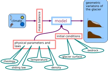
capture the complexity of glacier evolution. As depicted in Fig. 1, an ice flow model

solves the momentum and mass conservation equations for given initial and boundary conditions. The evolution of a glacier, i.e. the evolution of its surface geometry, is then fully determined by the ice flow and the climatic forcing. In what follows, we will only

10

consider isothermal glaciers, so that the climatic forcing reduces to a mass balance distribution at the surface of the glacier.

A right-handed (O, x, y, z) Cartesian coordinate system as depicted in Fig.2is used.

The surface and bedrock are defined as z=S(x, y, t) and z=B(x, y, t) respectively,

but the bedrock will be assumed to be a fixed boundary so thatz=B(x, y). The

ice-15

thickness is given byH=S−B. In what follows, the ice is considered as an isothermal

non-linear viscous incompressible material.

Due to ice incompressibility, the mass conservation equation can be expressed as:

∂vx

∂x +

∂v_y

∂y +

∂vz

∂z =0 . (1)

Here,v_x, v_y, v_z denote the components along the three directions of space of the

ve-20

locity vector v. The stress tensor τ splits into a deviatoric part τ′ and the isotropic

pressurep,

τi j =τ_{i j}′ +pδi j, (2)

where δ_{i j} is the Kronecker symbol. The constitutive relation, that links deviatoric

stresses to strain ratesǫ˙, is a power-law, referred to as the Glen’s flow law in glaciology:

(5)

TCD

2, 557–599, 2008

Title Page

Tables Figures

◭ ◮

Back Close

Full Screen / Esc

˙

ǫ_{i j} =A(T)τ⋆2τ_{i j}′ , (3)

whereA(T) is the deformation rate factor (hereafter reduced toAfor the isothermal ice

body, see Table2for its adopted value) andτ⋆is the second invariant of the deviatoric

stress tensor which is defined as:

5

τ⋆2=

1 2τ

′

i jτ

′

i j. (4)

The strain-rate components ˙ǫ_{i j} are defined from the velocity components as:

˙ ǫ_{i j} = 1

2 ∂vi

∂j +

∂v_j ∂i

!

, i , j =x, y, z. (5)

The force balance (quasi static equilibrium) in the three directions of space lead to the Stokes equations:

10

∂σx

∂x +

∂τxy

∂y +

∂τxz ∂z =0 , ∂τ_xy

∂x +

∂σ_y

∂y +

∂τ_yz ∂z =0 , ∂τ_xz

∂x +

∂τ_yz

∂y +

∂σ_z

∂z =ρg,

(6)

whereσi stands for τi i,g is the norm of the gravitational acceleration vector andρis

the glacier ice density (see Table2).

In temperate glaciers, in addition to the ice deformation, basal sliding contributes to the ice motion, but will be omitted in this study.

(6)

TCD

2, 557–599, 2008

Title Page

Tables Figures

◭ ◮

Back Close

Full Screen / Esc

At the stress-free upper surface (air-ice interface) the following kinematic equation applies for all points such thatz=S(x, y, t):

∂S ∂t +vx

∂S ∂x +vy

∂S

∂y −vz=a, (7)

whereais the mass balance function, considered as a vertical flux.

These equations finally lead to a complex system of five partial differential equations

5

with five independent unknowns (three terms of the velocity vector, one for isotropic pressure and another for the free surface elevation). Generally no analytical solution is

possible. Different models thus use different simplifications and numerical methods to

solve this set of equations.

3 Description of the three diff_{erent models}

10

In this inter-comparison study, three different models with different degrees of

com-plexity will be used, i.e. a simple zero-order SIA model (Sch ¨afer and Le Meur,2007),

a higher-order (HO) model (Pattyn,2003) and a full-Stokes (FS) model using the finite

element code Elmer (Elmer Manuals, CSC, 2006). In the interest of brevity and

be-cause it did not systematically succeed in converging, results from the HO model are

15

omited for some simulations. The aim of this section is to present in detail these three

different models.

3.1 SIA model

In the SIA formulation, important simplifications are introduced in the equations pre-sented above from a scale analysis by which the orders of magnitude of the various

20

variables are assessed. All variables are expressed as the product of a characteristic

value and a dimensionless quantity. Following the scale analysis from Hutter(1983)

(7)

TCD

2, 557–599, 2008

Title Page

Tables Figures

◭ ◮

Back Close

Full Screen / Esc

series of the aspect ratioǫas small parameter, assuming the aspect ratioǫis defined

as

ǫ= [H]

[L], (8)

and expressing the shallowness of the ice-sheet or glacier. [H] and [L] are respectively

a characteristic horizontal and vertical dimension of the studied ice-body. The

charac-5

teristical horizontal and vertical velocities ([V_L] and respectively [V_H]) scale in the same

way as the corresponding geometrical quantities,

ǫ= [VH]

[V_L]. (9)

However, as mentioned byBaral et al.(2001), the scaling of the velocities in Eq. (9) is

valid only for land based ice masses, but not for ice shelves.

10

All variables in the equations presented above are replaced by their corresponding

power series. In the zeroth-order SIA case only the remainingO-th-order terms are

kept. This implies that in the stress tensor all components vanish besidesτxz andτyz.

σ_x, σ_y, σ_z, τ_xy≪τ_xz, τ_yz (10)

A rigorous derivation has been developped byHutter(1983) and can also be found in

15

Baral et al.(2001). It is clear thatǫ<1 is a prerequisite for the SIA to apply and that the

smallerǫ, the more accurate is the approximation. Moreover,Morland (1984) shows

(8)

TCD

2, 557–599, 2008

Title Page

Tables Figures

◭ ◮

Back Close

Full Screen / Esc

Specifically, the SIA (0-th order) leads to

p(z)=ρg(z−S) , (11)

τ_{i z}=ρg(z−S)∂S

∂i , fori =x, y, (12)

∂v_⊥

∂z =−2A(ρg)

3₍_S₋_z₎3_|∇

⊥S|2∇⊥S, (13)

v_⊥=v_b+1

2A(ρg)

3

((S−z)4−H4)|∇_⊥S|2∇⊥S, (14)

5

wherev_bis the contribution of basal sliding if any,v_⊥=(v_x, v_y) stands for the two

hori-zontal velocity components and∇⊥ defines the horizontal components of the gradient

operator∇ (i.e. ∇⊥·=(∂·/∂x, ∂·/∂y)). Integration of the horizontal velocities from the

ice bottomBto the upper free surfaceS gives the horizontal fluxes as

q_⊥=v_bH−2

5A(ρg)

3_H5_|∇

⊥S|2∇⊥S. (15)

10

Vertical integration of the mass conservation Eq. (1) from B toS assuming the

kine-matic boundary condition (7) leads to a transport equation (Greve,1997):

∂H

∂t =a−∇⊥q⊥. (16)

Assuming∂B/∂t=0, this transport equation is transformed into a diffusion equation:

∂H

∂t =

∂S ∂t =a+

2(ρg)3 5

_∂

∂x

D∂S ∂x

+ ∂ ∂y

D∂S ∂y

, (17)

15

whereDis analogous to a diffusivity which reads

(9)

TCD

2, 557–599, 2008

Title Page

Tables Figures

◭ ◮

Back Close

Full Screen / Esc

when sliding is neglected.

Most of the time this equation is treated numerically with a semi-implicit (Sch ¨afer and

Le Meur, 2007) and in some cases with an over-implicit scheme (Hindmarsh,2001)

after being discretized according to a finite-difference method on a staggered regular

50 m×50 m grid.

5

3.2 Higher-order model

The model used here is the model developed byPattyn(2003). Two approximations

are applied on the initial set of equations presented above (Sect.2, Eqs. 1to7). The

major assumption consists of applying the hydrostatic approximation on the momentum equation. With this assumption, the third equation of the momentum set of Eqs. (6)

10

reduces to

∂σ_z

∂z =ρg, (19)

andσ_z can be directly obtained by integration.

Assuming a zero normal stress at the surface, the first two equations can be rewritten as follows:

15

∂ ∂x 2σ

′

x+σy′

+∂τ

′

x,y

∂y +

∂τ_xz′

∂z =ρg

∂S ∂x , ∂

∂y 2σ

′

y+σx′

+∂τ

′

x,y

∂y +

∂τ′yz

∂z =ρg

∂S ∂y .

(20)

In this model, the Glen’s law is expressed with the help of the second invariant of the

strain rate tensor ˙ǫ⋆defined as

˙ ǫ2_⋆= 1

(10)

TCD

2, 557–599, 2008

Title Page Abstract Introduction Conclusions References Tables Figures ◭ ◮ ◭ ◮ Back Close

Full Screen / Esc

The effective viscosity, defined asτ_{i j}′ =2ηǫ˙_{i j}, reads

η= 1

2A

−1

n (ǫ ⋆+ǫ˙0)

1−n

n , (22)

where ˙ǫ0is a small artificial number in order to prevent viscosity from becoming infinite

in case of zero strain-rate.

The second assumption of the model is that the horizontal gradients of the vertical

5

velocity are assumed to be small compared to the vertical gradient of the horizontal velocities: ∂v_z ∂x ≪ ∂v_x ∂z and ∂v_z ∂y ≪ ∂v_y

∂z . (23)

With this second assumption, the strain-rates ˙ǫxz and ˙ǫyz reduce to

˙ ǫ_xz = 1

2 ∂vx

∂z and ˙ǫyz =

1 2

∂vy

∂z . (24)

10

Combining the Glen’s flow law (22), the horizontal stress field Eqs. (20), the strain rate components and the equation of mass conservation (1) gives

∂

∂x 4ηǫ˙xx+2ηǫ˙yy

+ ∂

∂y 2ηǫ˙xy

+ ∂

∂z (2ηǫ˙xz) =ρg ∂S

∂x , (25)

∂

∂y 4ηǫ˙yy+2ηǫ˙xx

+ ∂

∂x 2ηǫ˙xy

+ ∂

∂z 2ηǫ˙yz

=ρg∂S

∂y . (26)

By replacing the strain-rates by their expression function of the velocity assuming

(11)

TCD

2, 557–599, 2008

Title Page Abstract Introduction Conclusions References Tables Figures ◭ ◮ ◭ ◮ Back Close

Full Screen / Esc

Eq. (24), these equations read:

4∂η ∂x ∂v_x ∂x + ∂η ∂y ∂v_x ∂y + ∂η ∂z ∂v_x

∂z +η 4

∂2v_x

∂x2 +

∂2v_x

∂y2 +

∂2v_x ∂z2

!

=ρg∂S

∂x −2

∂η ∂x ∂v_y ∂y − ∂η ∂y ∂v_y

∂x −3η

∂2v_y

∂x∂y , (27)

4∂η ∂y ∂v_y ∂y + ∂η ∂x ∂v_y ∂x + ∂η ∂z ∂v_y

∂z +η 4

∂2v_y

∂x2 +

∂2v_y

∂y2 +

∂2v_y

∂z2 !

=ρg∂S

∂y −2

∂η ∂y ∂v_x ∂x − ∂η ∂x ∂v_x

∂y −3η

∂2v_x

∂x∂y , (28)

5

where the effective viscosity is given by

η= 1

2A −1 n " _∂v x ∂x 2 + _∂v x ∂x 2

+∂vx ∂x ∂v_y ∂y +1 4 _∂v x ∂z 2 +1 4 ∂v_x ∂y + ∂vy ∂x !2 +1 4 ∂vy ∂z !2

+ǫ˙2₀





1−n

2n

. (29)

Solving these two linear equations leads to the horizontal velocity components. These

equations are treated as a pair of coupled linear equations withv_xandv_y as unknowns

10

andηis approximated from a previous iteration. The problem is solved in two steps: (i)

solving a linear set of equations using an estimate of the horizontal velocity field and

(ii) iterating the nonlinear part by updatingηwith new estimates ofv_xandv_y.

The vertical velocity is obtained by integration of the mass conservation equation.

To obtain the new surface elevation the kinematic Eq. (7) is rewritten as a diffusion

15

equation, the resulting sparse system is solved using a conjugate gradient method. For

(12)

TCD

2, 557–599, 2008

Title Page

Tables Figures

◭ ◮

Back Close

Full Screen / Esc

3.3 Full-Stokes model

The numerical solution of the FS equations is obtained using the Finite Element Method

based on the code Elmer (Elmer Manuals, CSC,2006). In the present case, the free

surface Eq. (7) and the Stokes Eq. (6) are coupled and solved iteratively using an implicit scheme during the increment time step.

5

3.3.1 Free surface equation

The non-integrated Eq. (7) is written in its discrete variational form:

∂Si ∂t

Z

V

φ_iΨd V +S_i

Z

V

v_H ·∇_⊥φ_iΨd V = Z

V

(a+v_z(S))Ψd V , (30)

whereS is developed as S(x, y, t)=φ_i(x, y)S_i(t) and where Ψ is a test function. S_i

stands for the discrete value of S at the i-th node of the domain. Stabilisation is

ob-10

tained by applying the Stabilised Method (Franca et al.,1992).

The vertical redistribution of the mesh nodes according to the moving boundary free surface is done by solving a linear elasticity equation.

3.3.2 Stokes equation

The mass conservation Eq. (1) and the Stokes Eqs. (6) are written in their variational

15

form

vi

Z

V ∇

ψiΦd V =0, (31)

−

Z

V

(piψi −τ′)·∇Φd V =−

I

∂V

(piψi −τ′)·n·Φd A+ρ

Z

V

gΦd V . (32)

A vector-like test functionΦ_{and the weight functions}_ψ_i _{are introduced, the left-hand}

side term in the momentum equation has been integrated by parts and reformulated

20

(13)

TCD

2, 557–599, 2008

Title Page

Tables Figures

◭ ◮

Back Close

Full Screen / Esc

The deviatoric stress tensorτ′ is expressed in terms of the strain-rate tensorǫ˙ with

the help of inversion of the power law (3). The non-Newtonian stress-strain relation in-troduces non-linearities into the system implying the application of an iteration scheme. The numerical solution of this system of equations is obtained either by the Stabilised

(Franca and Frey,1992) or the Residual Free Bubble method (Baiocchi et al.,1993).

5

For more details about the numeric in Elmer and the way the Stokes and free surface

equations are solved, the reader can refer to Le Meur et al. (2004); Zwinger et al.

(2007);Gagliardini and Zwinger(2008).

4 The diff_{erent glacier geometries}

Three simple-shaped synthetic glaciers are tested.

10

4.1 Flattened half-sphere

The first one, a flattened half-sphere on an inclined ramp (along the y-direction), is the

one that was already used byLe Meur et al.(2004) andSch ¨afer and Le Meur(2007).

This half-sphere has a radiusR of 500 m and is flattened with a factor 0.3 (see the

corresponding profile on Fig.3). Its center is at the origin. To asses the validity of the

15

SIA for increasing bedrock slopes, different slopespfrom 0 to 0.3 are used.

zbed=1000+p·y, (33)

zsurf=zbed+0.3 q

max(0, R2₋_x2₋_y2_{) ,} ₍₃₄₎

where all dimensions are expressed in meter.

4.2 Conic glacier

20

(14)

TCD

2, 557–599, 2008

Title Page

Tables Figures

◭ ◮

Back Close

Full Screen / Esc

photo and profile on Fig.4). The flat zone (radiusR=400 m) in the centre represents in

a very simple way the crater which is initially set free of ice and where the prescribed mass balance equals zero.

The ice-thickness is chosen to be uniform (40 m) over the whole glacier, except over the upper and bottom parts where it is assumed to reduce linearly to zero from

respec-5

tively 5500 to 5800 m and from 4880 m to 4800 m.

The bedrock slopepis varied from 0.3 to 0.8 as well. The real Cotopaxi glacier has

a mean slope of 0.55. The Cotopaxi geometry used is

zbed = (

5800 if px2₊_y2_≤_R_,

5800 +p(R−px2₊_y2₎ _otherwise, (35)

zsurf =  



zbed+40·

(5800−zbed)

300 if 5500≤z≤5800 ,

zbed+40·

(zbed−4800)

80 if 4800≤z≤4880 ,

z_bed+ 40 otherwise,

(36)

10

where all dimensions are expressed in meter.

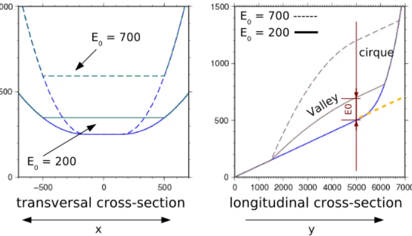
4.3 Valley glacier

The last glacier is also chosen close to a real case glacier, a typical mountain valley glacier (ex. Glacier d’Argenti `ere in the Mont Blanc range).

This glacier is composed of an ablation valley tongue (denoted V in the formulas

15

below) and a cirque (Cin the formulas). y is the direction of the ice-flow (the origin is

somewhere below the snout), x is orthogonal to this direction with x=0 at the centre

of the glacier. At the interface (y=5000 m) of these two parts of the glacier, the

ice-thickness is given by the parameterE0 and is varied from 100 m to 700 m in order to

modify the aspect ratio of the glacier (aspect ratios ranging from 0.1 to 0.7).

20

In the valley part, the bedrock is the superposition of a linear down-sloping function

in the direction of ice flow (slope 0.1) and a parabolic function inx (orthogonal to the

(15)

TCD

2, 557–599, 2008

Title Page

Tables Figures

◭ ◮

Back Close

Full Screen / Esc

see formulas below and Fig.5.

z_bed_V(x, y)=E₀+0.1y+E_x(x) , (37)

with

E_x(x)=

 



E₀·

|x|−150 500

2 · −1

,if|x|>150 ,

−E₀ otherwise.

(38)

In the upper part of the glacier the bedrock is given by a 3rd degree function

5

zbed_C =E0+Ex(x)+c·y3+d·y2+e·y+f , (39)

where the different parameters are defined by the following boundary conditions:

zbed_V(x,5000)=zbed_C(x,5000) , (40)

∂zbed_V(x, y)

∂y |(0,5000)=

∂zbed_C(x, y)

∂y |(0,5000), (41)

∂2zbed_V(x, y)

∂y2 |(0,5000)=

∂2zbed_C(x, y)

∂y2 |(0,5000), (42)

10

zbed_C(0,7000)=1700 . (43)

For the upper part (cirque) this initial surface reads:

zsurf_C =E0+0.1y, (44)

whereas for the lower part (valley), the following quadratic reduction of the ice-thickness is chosen;

15

zsurf_V =max(zbed,(ay2+by+c)) , (45)

in which the parameters are chosen for the surface function to be a one time diff

eren-tiable function at the interface between the two parts of the glacier and for the snout

to be positioned aty=1500 m. These different surfaces (bedrock, ice) are depicted in

Fig.5.

(16)

TCD

2, 557–599, 2008

Title Page

Tables Figures

◭ ◮

Back Close

Full Screen / Esc

Interactive Discussion 5 Simulations and results

Simulations with different degrees of complexity are carried out, that is diagnostic and

prognostic simulations, as well as simulations with and without mass balance. These

different types of simulations are performed to assess separately the influence of the

viscous ice deformation and the effect of mass balance. An overview of the different

5

simulations is given in Table1.

For all the simulations, the same numerical values as given in Table2are adopted.

They are typical values for an alpine glacier (see for instanceLliboutry,1965).

5.1 Diagnostic simulations

In the diagnostic simulations, velocity distributions of the different models are compared

10

for given and fixed geometries. In all simulations an overestimation of the velocities over the whole ice-body by the SIA model was observed. In most cases, there was a good agreement between HO and FS velocities. These observations are illustrated in

the following paragraphs for the different glaciers.

5.1.1 Flattened half-sphere glacier

15

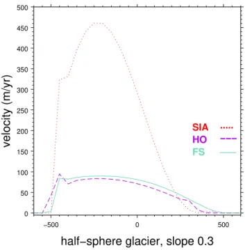
In Fig.6, the norm of the surface velocity vector is shown over the symmetry axis for the

different models in the case of a bedrock slope of 0.3. An overestimation with the SIA

appears clearly whereas the HO model leads to a smaller amplitude underestimation.

In the case of the flattened half-sphere, there was no real difference regarding this

over(under)estimation seen for different bedrock slopes. Probably this is due to the

20

(17)

TCD

2, 557–599, 2008

Title Page

Tables Figures

◭ ◮

Back Close

Full Screen / Esc

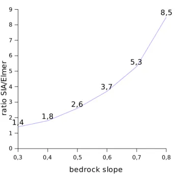
5.1.2 Conic glacier

In the case of the conic glacier, the dependence of the validity of the SIA on the bedrock

slope is clearly observable. In Fig.7, the ratio between SIA and FS velocities is shown

for the radial component with different bedrock slopes (the almost uniform velocities in

the region where the ice-thickness is 40 m are here considered). The overestimation

5

of the velocities produced by the SIA model, increases with increasing bedrock slope.

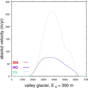
5.1.3 Valley glacier

For this geometry, the over-implicit scheme has been used for the SIA model, allow-ing a better convergence with bigger time-steps (for diagnostic as well as prognostic simulations).

10

In the same way, a degradation of the SIA with the aspect ratio of the ice body is

detectable in the case of the valley glacier. In Fig. 8, the evolution of the norm of

the surface velocity vector along the symmetry axis (x=0) is shown for two different

ice-thicknesses.

As for the other geometries, the HO model leads to an underestimation of velocities

15

(hardly visible in the figure due to the scale).

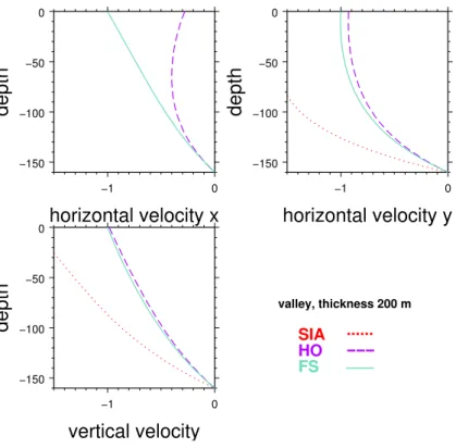
In addition, this type of geometry indicates that models not resolving the FS equa-tions not only disagree in terms of amplitude, but there can be also velocity components

that are not distinguished at all with some models. This is illustrated in Fig.9, where the

vertical profiles of the different velocity components in one specific point, not located

20

on the symmetry axis, are shown. The velocity in the x-direction is not distinguished with the SIA model. In the SIA the ice-flow occurs always along the highest slope, the

velocity in the x-direction equals zero, asd S/dx=0. This reiterates the weakness of

(18)

TCD

2, 557–599, 2008

Title Page

Tables Figures

◭ ◮

Back Close

Full Screen / Esc

5.1.4 Some remarks on the influence of sliding

No experiences with sliding are presented here. Nevertheless several simulations with

different Weertman-type sliding laws (Weertman, 1964) have been conducted. The

main result of these simulations is that qualitatively the agreement between the SIA and the FS model is in the most cases better than without sliding. This result is surprising as

5

a degradation of the SIA is expected as the spatial transmission of the stress gradients

which is neglected in the SIA becomes more important (Gudmundsson,2003).

In the chosen simulations the better agreement can be explained by the fact that the total velocity is dominated by the sliding velocity compared to the deformation velocity and very good agreement for the basal velocities is achieved between both models.

10

5.2 Prognostic simulations

In the prognostic simulations we compare the final velocity distributions of the different

models as well as the deformation of the surface under the ice-flow and mass balance

(mass balance is applied only in Sect.5.3). As in the diagnostic case, in all simulations

the SIA model overestimates velocities, but this overestimation decreases with time.

15

This decrease of the overestimation can be explained by a negative feedback.

Initial (diagnostic) velocities are overestimated within the SIA which leads to extra de-formation of the ice. This in return gives a thinner and flatter glacier compared with the FS approach which is assumed to be close to reality. As SIA-velocities are proportional to ice-thickness and surface slope (raised to the 4th and 3rd powers, respectively), they

20

(19)

TCD

2, 557–599, 2008

Title Page

Tables Figures

◭ ◮

Back Close

Full Screen / Esc

5.2.1 Simulations where no mass balance is applied

Flattened half-sphere glacier

For this geometry, no steady state simulation is possible under zero mass balance. The simulations were thus conducted over a period of 50 years, a period long enough

to observe different behaviours of the different models and short enough to deal with

5

reasonable calculation time. In terms of velocity the same observations as in the diag-nostic case are made, i.e. overestimation by the SIA model and small underestimation by the HO model. However, the longer the simulation, the better is the agreement

be-tween the three models. Figure10showing the final vertical profile of the norm of the

velocity vector at point (x, y)=(300,−250) for the prognostic simulation (left of figure)

10

as well as for a diagnostic simulation (right of figure) illustrates the better agreement in the case of a prognostic simulation. In both cases velocities are normalized to the corresponding FS surface velocities. The initial ratio between the SIA and the FS ve-locities decreases from about 4 (diagnostic) to nearly 1 (at the end of the prognostic simulations).

15

The observations made on the surface deformation are in agreement with those ob-served with velocities. The SIA glacier is too thin and too long (because has undergone

too much deformation), whereas the HO glacier is not deformed enough (Fig.11, thick

lines).

Conic glacier 20

In the same way as for the flattened half-sphere glacier, the simulation time was fixed to 50 years in the case of simulations where no mass balance is applied. As for the velocities, a degradation of the agreement for the terminus position between the SIA

and the FS models is observed with increasing bedrock slopes (Fig.12, bottom part

of the figure). The HO model simulations are sometimes missing because of problems

25

(20)

TCD

2, 557–599, 2008

Title Page

Tables Figures

◭ ◮

Back Close

Full Screen / Esc

model is rather good.

The previously mentioned negative feedback is investigated in more details with this

glacier. Figure13shows the absolute differences for the surface altitude (dotted line)

and the vertical velocity (full line) between the SIA and the FS model as a function of

time during the 50 years of simulation. The difference in velocity is decreasing

asymp-5

totically to a small value close to zero, whereas the difference for the surface altitude

increases asymptotically to a given value. Thus, for a sufficient long simulation, the

SIA velocities get close to FS velocities and the discrepancy in terms of ice-thickness stays constant, as the error on the ice-thickness represents the cumulative errors on velocities.

10

The simulation duration needed to achieve these asymptotic values depends on the bedrock slope, the larger the slope the faster the discrepancy becomes constant (not shown).

Valley glacier

Some simulations with the HO model are missing as the required simulation time

ap-15

peared too long. Simulations with the valley glacier confirm the observations made with the other glacier types.

Given the negative feedback exposed by the previous simulations, it appeared worth-while to pursue by changing the simulation time as a function of the initial ice-thickness,

i.e. the parameterE0. The simulation duration was determined according to a criterion

20

based on surface deformation during the simulation. The different simulations with the

parameterE0are run until the same amount of deformation is achieved, i.e. when the

ice-thickness at the middle of the junction between valley and cirque part (0 m, 5000 m)

has reduced to 65% of its initial value. The only exception is forE₀=100 m for which the

simulation was stopped after 100 years because of too small an amount of deformation.

25

As can be seen from Fig.14, one additional observation can be made with this kind

(21)

TCD

2, 557–599, 2008

Title Page

Tables Figures

◭ ◮

Back Close

Full Screen / Esc

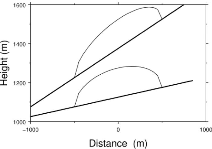
model eventually appears with large initial thicknesses. At the end of the prognostic simulation, the figure shows a convex shape for the FS model, whereas the surface becomes concave with the SIA.

5.3 Prognostic simulations where mass balance is included

Prognostic simulation have also been carried out with prescribed mass balance fields.

5

In the case of the flattened half-sphere glacier, a spherical mass balance distribution

aS was chosen with 5 m of ice in the centre (shifted downhill by 250 m compared to the

centre of the ice-body). This distribution remains constant in time.

a_S=

(

5·pR2₋_x₋2₋₍_y₋₂₅₀₎2 _ifp_x2₊₍_y₋₂₅₀₎2_≤_R_,

−5· px2₊₍_y₋₂₅₀₎2₋_R2 _otherwise. (46)

In the case of the conic glacier, a linear dependency with altitude was chosen with

10

a change in the regression coefficient at the equilibrium line (ELA=5100 m). However

for simplicity knowing the relatively thin ice-thickness the mass balance distribution

aC was kept constant in time and calculated according to the initial surface altitude.

This distribution is motivated by observations made at another nearby volcano glacier (Antizana).

15

a_C =

 



22 ×10−3·(surf_ini−E LA) ifz_surf

ini ≤E LA,

1.14×10−3·(surf_ini−E LA) ifz_surf

ini > E LA,

0 in the crater.

(47)

In the case of the valley glacier a linear dependency with altitude was chosen as well

for the mass balance distributionaV (with a coefficient of 0.004 m−1as observed on the

Glacier d’Argenti `ere in France).

a_V =0.004 (zsurf_ini−ELA). (48)

20

(22)

TCD

2, 557–599, 2008

Title Page

Tables Figures

◭ ◮

Back Close

Full Screen / Esc

rock slopes around the upper cirque. For convenience the mass balance was calcu-lated once again accordingly to the initial surface altitude.

Apart from the case of the valley glacier, all simulations achieve a steady state sur-face. For the valley glacier the same simulation time as with zero mass balance was chosen because this duration implies the same amount of deformation.

5

In all simulations a good agreement for the snout position was observed (see Figs.11

and12), but not necessarily for the entire glacier geometry. The good agreement for the

snout position is explained probably just by the fact that the geometries reduce easily to a 2-D geometry (i.e. a problem with two dimensions in space). In 2-D the snout position in a steady state is fully determined by the mass balance distribution (which is

10

kept constant in all conducted experiences) and the upper border of the glacier, as the total surface mass balance integrated on the glacier surface is equal to zero.

In the case of the valley glacier an interesting point regarding time evolution has been brought up. With the FS model the glacier systematically retreats from the very start. With the SIA model for large thicknesses, the glacier first re-advances due to high

15

deformation rates, and then retreats because of the negative mass balance field. In

some situations the overestimation of deformation of the SIA can overcome the effect

of a mass balance field and completely change the behaviour.

5.4 Comparison of CPU time

As one example for comparison of CPU time, the CPU time necessary for a simulation

20

with the different models was investigated with the flattened half-sphere (slope 0.2).

This work does not intend to be an exhaustive study on the CPU requirements with the

different models. Instead, the different models as they currently exist are used, i.e.

with-out putting any emphasis on optimisation of the codes, the convergence parameters, initial conditions, time steps, spatial grid steps, etc. Nevertheless, all these parameters

25

have been varied in order to get an idea on the effect on the total CPU time. The aim of

this section is thus just to get in a fast and simple way an overall idea of the differences

(23)

TCD

2, 557–599, 2008

Title Page

Tables Figures

◭ ◮

Back Close

Full Screen / Esc

in this study.

Two different scenarios have been chose; a diagnostic simulation and a prognostic

simulation of 10 years without sliding and with zero mass balance.

5.4.1 Diagnostic velocity field

Some interesting observations with the FS model have been made for the CPU time,

5

which (i) does not increase linearly with calculation precision, (ii) increases nearly lin-early with the number of grid nodes and (iii) is very sensitive to the initial conditions. In the case of the HO model, CPU time increases more than linearly with the number of grid-points, but initial conditions are less important.

Taking into account the different parameter sets that are not detailed here, a ratio

10

ofO(10 000) was found between the FS model and the SIA model, the ratio between

the FS model and the HO model was only between O(10) and O(100) and the one

between the HO model and the SIA solution wasO(100).

Specifically, 0.06 s have been needed for the SIA model, between 17 and 28 s for

the HO model (depending on different convergence parameters and initial conditions

15

chosen) and between 4 and 18 min for the FS model (also depending on different

pa-rameters and initial conditions).

5.4.2 Prognostic simulation

No linear dependency on the time-step was found both for the FS and HO models.

Increasing of the time-step by a factor of 2 led to an increase of a factor of 1.3 in

20

calculation time for the FS model and to a factor of 2.3 for the HO model.

In this case the computing time was between 0.22 and 0.39 s for the SIA model,

between 30 and 108 min for the HO model and between 2.5 and 4 h for the FS model

(in all cases for different parameter sets chosen).

Taking into account the different simulations, the ratio for the CPU time between

25

(24)

TCD

2, 557–599, 2008

Title Page

Tables Figures

◭ ◮

Back Close

Full Screen / Esc

remainsO(10 000) and the one between the HO model and the SIA increases to nearly

O(10 000) as well.

The large difference between the results on diagnostic and prognostic simulations is

explained by the high sensitivity of the FS model to initial conditions. The calculation of the diagnostic velocity field takes disproportionally more time compared to the next

5

time steps; whereas the HO model takes nearly the same time for all time steps – the

initial one included. This explains the different ratios for the two types of simulations.

Finally we can conclude that the saving of CPU time with an SIA model is important, but taking a HO model instead of a FS model will not necessarily bring an advantage in CPU time. The latter case has to be investigated further for each given application.

10

6 Conclusions

The inter-comparison here uses three different models, a Shallow Ice Approximation

(SIA) model, a higher-order (HO) model and a full-Stokes (FS) one. Different synthetic

shaped glaciers have been used with different aspect ratios and bedrock slopes.

SIA models are frequently used for modeling large ice masses because of their huge

15

advantages in terms of CPU time and implementation/development facilities. However, this approximation is only valid for ice bodies with a small aspect ratio and a weak

bedrock slope. In the SIA, longitudinal stresses (σ_x,y,z′ ) are neglected which prevents

stress transmission within grid points and therefore makes the theory local. Glacier evolution at a given point of the glacier thus only depends upon the local topography

20

without including any interactions from the neighboring points. This approximation is certainly not very realistic, especially in the case of a non regular surface or bed

to-pography. Horizontal shear stress (τxy′ ) is neglected as well in this theory, which is

especially not justified in the case of a glacier deeply channelled in a valley, where the importance of such stresses is obvious and for example clearly visible with the bending

25

of the Forbes bands.

(25)

TCD

2, 557–599, 2008

Title Page

Tables Figures

◭ ◮

Back Close

Full Screen / Esc

can be observed on velocity fields as well as on evolved glacier geometries. This over-estimation is partly a consequence of the local character of the model due to the lack of longitudinal coupling. In contrast, the HO model leads to a small underestimation. It is also obvious that the smaller the aspect ratio, the better the SIA results as for instance

also shown inLe Meur et al.(2004).

5

More specifically, the following observations are made with the different simulation

types: in the diagnostic simulations a huge disagreement between the SIA and the other models has been observed. This disagreement increases with the aspect ratio (valley glacier) and the bedrock slope (conic glacier). In the prognostic simulations the agreement for velocities is much better because of a negative feedback obtained with

10

the SIA. Nevertheless, the overestimation of deformation is still noticeable from the time-dependent geometry evolution.

Mass-balance essentially affects the snout position and a very good agreement

be-tween the different models was obtained for this observable, however, a disagreement

in terms of surface geometry remains. In some cases, even the glacier behaviour can

15

change, e.g. an initial advance rapidly followed by a retreat with the SIA model contrary to the FS model which continuously retreats from the start.

In terms of comparison of CPU time, the advantage of the SIA model has clearly been shown. But the switch between a HO and a FS model does not necessarily bring a big advantage in term of calculation time.

20

Thus, the SIA seems to be a good approximation in the case of prognostic simula-tions with small aspect ratios and small bedrock slopes. The mass balance does not

have a real effect on this issue but can nevertheless affect the global behaviour.

As a next step, it would be interesting to make some more comparisons on prognostic simulations, not only by comparing final velocities and surfaces, but by comparing the

25

(26)

TCD

2, 557–599, 2008

Title Page

Tables Figures

◭ ◮

Back Close

Full Screen / Esc

Interactive Discussion References

Baiocchi, C., Brezzi, F., and Franca, L. P.: Virtual bubbles and the Galerkin least squares method, Comp. Meths. Appl. Mech. Engrg., 105, 125–141, 1993. 569

Baral, D. R., Hutter, K., and Greve, R.: Asymptotic theories of large-scale motion, temperature, and moisture distribution in land-based polythermal ice sheets: A critical review and new

5

developments, Appl. Mech. Rev., 54, 2001. 563

Elmer Manuals, CSC:http://www.csc.fi/elmer/, 2006. 562,568

Franca, L. P. and Frey, S. L.: Stabilized finite element methods: II. the incompressible Navier-Stokes equations, Comput. Methods Appl. Mech. Eng., 99, 209–233, 1992. 569

Franca, L. P., Frey, S. L., and Hughes, T. J. R.: Stabilized finite element methods: I. application

10

to the advective-diffusive model, Comput. Methods Appl. Mech. Eng., 95, 253–276, 1992. 568

Gagliardini, O. and Zwinger, T.: The ISMIP-HOM benchmark experiments performed using the Finite-Element code Elmer, The Cryosphere, 2, 67–76, 2008. 569

Greuell, W.: Hintereisferner, Austria: mass-balance reconstruction and numerical modelling of

15

the historical lenght variation, J. Glaciol., 38, 233–244, 1992. 559

Gudmundsson, G. H.: Transmission of basal variability to a glacier surface, J. Geophys. Res., 108, 2253, doi:10.1029/2002JB002107, 2003. 574

Greve, R.: A Continuum-Mechanical Formulation for Shallow Polythermal Ice Sheets, Philo-sophical Transactions: Mathematical, Physical and Engineering Sciences, 355, 921–974,

20

1997. 564

Hindmarsh, R.: Notes on basic glaciological computational methods and algorithms, Contin-uum mechanics and applications in geophysics and the environment (A 02-10739 01-46), Berlin, Heidelberg and New York, Springer-Verlag, pp. 222–249, 2001.565

Hindmarsh, R.: A numerical comparison of approximations to the Stokes equations used in ice

25

sheet and glacier modeling, J. Geophys. Res., 109, 1–15, 2004.559

Hubbard, A.: The Verification and Significance of Three Approaches to Longitudinal Stresses in High-Resolution Models of Glacier Flow, Geografiska Annaler. Series A, Physical Geography, 82, 471–487, 2000.558

Hutter, K.: Theoretical Glaciology: material science of ice and the mechanics of glaciers

30

(27)

TCD

2, 557–599, 2008

Title Page

Tables Figures

◭ ◮

Back Close

Full Screen / Esc

Le Meur, E. and Vincent, C.: A two-dimensional shallow ice flow model of glacier de Saint Sorlin, France, J. Glaciol., 49, 527–538, 2003. 558

Le Meur, E., Gagliardini, O., Zwinger, T., and Ruokolainen, J.: Glacier flow modelling: a com-parison of the Shallow Ice Approximation and the full-Stokes solution, CRAS Physique, 5, 709–422, 2004. 559,569,581

5

Leysinger Vieli, G. J.-M. C. and Gudmundsson, G. H.: On estimating length fluctua-tions of glaciers caused by changes in climatic forcing, J. Geophys. Res., 109, F01007, doi:10.1029/2003JF000027, 2004.558,559

Lliboutry, L.: Trait ´e de glaciologie, Glaciers – Variations du climat – Sols gel ´es, Masson & Cie Editeurs, 1965. 572

10

Morland, L. W.: Thermomechanical balance of ice sheet flows, Geophys. Astrophys. Fluid Dynam., 29, 237–266, 1984.562,563

Pattyn, F.: A new three-dimensional higher-order thermomechanical ice sheet model: Basic sensitivity, ice stream development, and ice flow across subglacial lakes, J. Geophys. Res., 108, 2382, doi:10.1029/2002JB002329, 2003. 562,565,567

15

Pattyn, F. and Payne, T.: Ice Sheet Model Intercomparison Project: Benchmark experiments for numerical Higher-Order ice-sheet Models,http://homepages.ulb.ac.be/∼_{fpattyn/ismip/, 2006.}

559

Pattyn, F., Perichon, L., Aschwanden, A., Breuer, B., de Smedt, B., Gagliardini, O., Gudmunds-son, G. H., Hindmarsh, R., Hubbard, A., JohnGudmunds-son, J. V., Kleiner, T., Konovalov, Y., Martin,

20

C., Payne, A. J., Pollard, D., Price, S., R ¨uckamp, M., Saito, F., Souˇcek, O., Sugiyama, S., and Zwinger, T.: Benchmark experiments for higher-order and full Stokes ice sheet models (ISMIP-HOM), The Crysosphere Discuss., 2, 111–151, 2008. 559

Sch ¨afer, M. and Le Meur, E.: Improvements of a 2D-SIA ice flow model; application to the Saint Sorlin glacier, France, J. Glaciol., 53, 713–722, 2007. 562,565,569

25

Weertman, J.: The theory of glacier sliding, J. Glaciol., 39, 287–303, 1964.574

(28)

TCD

2, 557–599, 2008

Title Page

Tables Figures

◭ ◮

Back Close

Full Screen / Esc

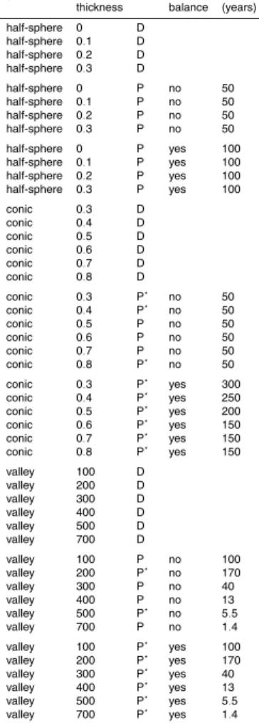
Table 1.Overview of simulations. D (P) stands for Diagnostic (Prognostic). Simulations with⋆ are missing for the HO model.

glacier slope or D/P mass duration thickness balance (years) half-sphere 0 D

half-sphere 0.1 D half-sphere 0.2 D half-sphere 0.3 D

half-sphere 0 P no 50 half-sphere 0.1 P no 50 half-sphere 0.2 P no 50 half-sphere 0.3 P no 50 half-sphere 0 P yes 100 half-sphere 0.1 P yes 100 half-sphere 0.2 P yes 100 half-sphere 0.3 P yes 100 conic 0.3 D

conic 0.4 D conic 0.5 D conic 0.6 D conic 0.7 D conic 0.8 D

conic 0.3 P⋆ no 50 conic 0.4 P⋆ _no ₅₀

conic 0.5 P no 50 conic 0.6 P no 50 conic 0.7 P no 50 conic 0.8 P⋆ _no ₅₀

conic 0.3 P⋆ _yes ₃₀₀

conic 0.4 P⋆ _yes ₂₅₀

conic 0.5 P⋆ _yes ₂₀₀

conic 0.6 P⋆ _yes ₁₅₀

conic 0.7 P⋆ yes 150 conic 0.8 P⋆ _yes ₁₅₀

valley 100 D valley 200 D valley 300 D valley 400 D valley 500 D valley 700 D

valley 100 P no 100 valley 200 P⋆ _no ₁₇₀

valley 300 P no 40 valley 400 P no 13 valley 500 P⋆ no 5.5 valley 700 P no 1.4 valley 100 P⋆ _yes ₁₀₀

valley 200 P⋆ yes 170 valley 300 P⋆ _yes ₄₀

valley 400 P⋆ yes 13 valley 500 P⋆ _yes ₅_.₅

(29)

TCD

2, 557–599, 2008

Title Page

Tables Figures

◭ ◮

Back Close

Full Screen / Esc

Table 2.Numerical values of the parameters adopted for the all the simulations.

g=9.81 m s−2 gravity constant

(30)

TCD

2, 557–599, 2008

Title Page

Tables Figures

◭ ◮

Back Close

Full Screen / Esc

(31)

TCD

2, 557–599, 2008

Title Page

Tables Figures

◭ ◮

Back Close

Full Screen / Esc

(32)

TCD

2, 557–599, 2008

Title Page

Tables Figures

◭ ◮

Back Close

Full Screen / Esc

Interactive Discussion 1000

1200 1400 1600

Height (m)

−1000 0 1000

Distance (m)

(33)

TCD

2, 557–599, 2008

Title Page

Tables Figures

◭ ◮

Back Close

Full Screen / Esc

5500

height (m)

0 500 1000 1500 2000 2500 distance (m) to the center

surface

bed

(34)

TCD

2, 557–599, 2008

Title Page

Tables Figures

◭ ◮

Back Close

Full Screen / Esc

(35)

TCD

2, 557–599, 2008

Title Page

Tables Figures

◭ ◮

Back Close

Full Screen / Esc

50 100 150 200 250 300 350 400 450 500

velocity (m/yr)

−500 0 500

half−sphere glacier, slope 0.3

HO −−−

FS ___

SIA ...

(36)

TCD

2, 557–599, 2008

Title Page

Tables Figures

◭ ◮

Back Close

Full Screen / Esc

(37)

TCD

2, 557–599, 2008

Title Page

Tables Figures

◭ ◮

Back Close

Full Screen / Esc

50 100 150 200 250 300

absolut velocity (m/yr)

0 1000 2000 3000 4000 5000 6000 7000

valley glacier, E ₀ = 300 m

HO −−−

FS ___

SIA ...

(38)

TCD

2, 557–599, 2008

Title Page

Tables Figures

◭ ◮

Back Close

Full Screen / Esc

Interactive Discussion −150

−100 −50 0

depth

−1 0

horizontal velocity x

−150 −100 −50 0

depth

−1 0

horizontal velocity y

−150 −100 −50 0

depth

−1 0

vertical velocity

valley, thickness 200 m

SIA ...

FS ___

HO −−−

(39)

TCD

2, 557–599, 2008

Title Page

Tables Figures

◭ ◮

Back Close

Full Screen / Esc

Interactive Discussion −50

0

depth (m)

0 1

velocity (m/yr) P

−100 −50 0

depth (m)

0 1 2 3 4 5

velocity (m/yr) D

(40)

TCD

2, 557–599, 2008

Title Page

Tables Figures

◭ ◮

Back Close

Full Screen / Esc

1100 1200 1300 1400 1500 1600

height (m)

−1000 −500 0 500

half−sphere glacier, slope 0.3

thick lines: with zero mass balance thin lines: with mass balance

HO −−−

FS ___

SIA ...

(41)

TCD

2, 557–599, 2008

Title Page

Tables Figures

◭ ◮

Back Close

Full Screen / Esc

4600 4700 4800 4900 5000

snout position

0.2 0.3 0.4 0.5 0.6 0.7 0.8 0.9 slope

with mass balance

no mass balance

SIA ...

FS ___

HO −−−

(42)

TCD

2, 557–599, 2008

Title Page

Tables Figures

◭ ◮

Back Close

Full Screen / Esc

5 10

absolut difference (vertical velocity, m/yr)

0 5 10 15 20 25 30 35 40 45 50

time (yr)

0 5 10

absolut difference (surface, m)

slope 0.8

(43)

TCD

2, 557–599, 2008

Title Page

Tables Figures

◭ ◮

Back Close

Full Screen / Esc

300 350 400

height (m)

−500 0 500

valley glacier, E 0 = 100 m 295

300 305

−400 −200 0 200 400

HO −−− FS ___ SIA ...

250 300 350 400 450 500 550 600 650 700 750 800 850 900 950 1000 1050 1100 1150 1200 1250 1300

height (m)

−500 0 500

valley glacier, E 0 = 700 m 690

695 700 705 710 715

−600−400−200 0 200 400 600

HO −−− FS ___ SIA ...