www.geosci-model-dev.net/7/1901/2014/ doi:10.5194/gmd-7-1901-2014
© Author(s) 2014. CC Attribution 3.0 License.
A multiresolution spatial parameterization for the estimation of
fossil-fuel carbon dioxide emissions via atmospheric inversions
J. Ray1, V. Yadav2, A. M. Michalak2, B. van Bloemen Waanders3, and S. A. McKenna4
1Sandia National Laboratories, P.O. Box 969, Livermore, CA 94551, USA 2Carnegie Institution for Science, Stanford, CA 94305, USA
3Sandia National Laboratories, P.O. Box 5800, Albuquerque, NM 87185-0751, USA
4IBM Research, Smarter Cities Technology Centre, Bldg 3, Damastown Industrial Estate, Mulhuddart, Dublin 15, Ireland
Correspondence to:J. Ray ([email protected])
Received: 28 December 2013 – Published in Geosci. Model Dev. Discuss.: 6 February 2014 Revised: 2 July 2014 – Accepted: 18 July 2014 – Published: 3 September 2014
Abstract. The characterization of fossil-fuel CO2 (ffCO2)
emissions is paramount to carbon cycle studies, but the use of atmospheric inverse modeling approaches for this pur-pose has been limited by the highly heterogeneous and non-Gaussian spatiotemporal variability of emissions. Here we explore the feasibility of capturing this variability using a low-dimensional parameterization that can be implemented within the context of atmospheric CO2 inverse problems
aimed at constraining regional-scale emissions. We construct a multiresolution (i.e., wavelet-based) spatial parameteriza-tion for ffCO2emissions using the Vulcan inventory, and
ex-amine whether such a parameterization can capture a realis-tic representation of the expected spatial variability of actual emissions. We then explore whether sub-selecting wavelets using two easily available proxies of human activity (im-ages of lights at night and maps of built-up areas) yields a low-dimensional alternative. We finally implement this low-dimensional parameterization within an idealized inver-sion, where a sparse reconstruction algorithm, an extension of stagewise orthogonal matching pursuit (StOMP), is used to identify the wavelet coefficients. We find that (i) the spa-tial variability of fossil-fuel emission can indeed be repre-sented using a low-dimensional wavelet-based parameteriza-tion, (ii) that images of lights at night can be used as a proxy for sub-selecting wavelets for such analysis, and (iii) that implementing this parameterization within the described in-version framework makes it possible to quantify fossil-fuel emissions at regional scales if fossil-fuel-only CO2
observa-tions are available.
1 Introduction
The characterization of fossil-fuel CO2 (ffCO2) emissions
is paramount to carbon cycle studies. ffCO2 emissions are
the largest net carbon flux at the atmosphere–surface in-terface (Friedlingstein et al., 2006) and spatially disaggre-gated (or gridded) ffCO2 emissions form a critical input
into general circulation and integrated assessment models (Andres et al., 2012). An understanding of fossil-fuel emis-sions is clearly necessary for characterizing the anthro-pogenic climate impact. In addition, a process-level under-standing of the terrestrial carbon sink requires the quantifi-cation of terrestrial biospheric fluxes at fine spatiotemporal scales, which, in turn, requires the differentiation between anthropogenic and biospheric fluxes at those scales.
Gridded inventory estimates of ffCO2emissions can be
de-rived using socio-economic data (Oda and Maksyutov, 2011; Rayner et al., 2010), and such “bottom-up” estimates have been proposed as a means of monitoring international agree-ments aimed at mitigating ffCO2 emissions (Pacala et al.,
2010). Gridded inventory estimates are derived from ffCO2
budgets and produced by a few institutions; see Andres et al. (2012) for a list. These budgets are compiled from national and provincial statistics on fossil-fuel production and con-sumption. These large-scale estimates can then be down-scaled to finer spatiotemporal scales using easily observed proxies of human activity (and consequently ffCO2
approaches to the fine-scale bottom-up estimation of ffCO2
emissions have also begun to emerge, including, for exam-ple, the Vulcan inventory that includes estimates for the US at a 10 km and hourly resolution for 2002 (http://vulcan.project. asu.edu; Gurney et al., 2009). Such approaches rely on de-tailed reporting and monitoring data, which are not currently available for many regions of the world.
Although inventory estimates provide a key tool in the understanding of anthropogenic CO2 emissions, their
accu-racy at large scales depends on the accuaccu-racy of reported national consumption data, e.g., the error in ffCO2
emis-sions from China lies in the 15–20 % range (Gregg et al., 2008). When evaluated at finer spatiotemporal scales, their accuracy also depends on the method used to disaggregate national/provincial ffCO2 emission budgets to finer spatial
scales. Pregger et al. (2007) showed that two 0.5◦ invento-ries for Western Europe, for 2003, differed at the grid-cell level by 20 %, with a standard deviation of 40 %; at finer res-olutions, the disagreement worsened. Sources of errors in in-ventories are discussed in detail in Andres et al. (2012), Rau-pach et al. (2009) and Rayner et al. (2010). These uncertain-ties lead to frequent corrections of sub-national inventories of combustion products (Streets et al., 2006) and model predic-tions of CO2concentrations that disagree with observations
locally (Brioude et al., 2012).
Given both the benefits, and the limitations, of inventory-based estimates, interest has emerged in the development of “top-down” estimates of ffCO2 emissions. These estimates
rely on attributing the observed variability in CO2 and
re-lated trace gas concentrations in the atmosphere to the under-lying fossil-fuel emissions, through the application of statis-tical atmospheric inversion methods. Some of the proposed approaches, (e.g., Turnbull et al., 2011) have relied on obser-vations of114CO2measurements or other non-CO2tracers.
One challenge with these approaches, however, is a combina-tion of the limited number of available observacombina-tions and the need to understand emission ratios for any co-emitted tracers. Atmospheric inversions relying on atmospheric CO2
mea-surements, on the other hand, have primarily targeted bio-spheric CO2fluxes, often by first pre-subtracting the
fossil-fuel influence calculated from an inventory; see Ciais et al. (2010) for a review of atmospheric inversion methods. The measurements then consist of CO2 concentration obtained
from in situ or remote-sensing observations, and estimates are obtained at a variety of spatiotemporal resolutions for ei-ther global or regional domains. The statistical approaches applied typically rely on Gaussian assumptions for flux resid-uals from prior estimates or other spatiotemporal patterns. In-vestigations aimed at the estimation of ffCO2emissions are
less common because (1) measurements of ffCO2
concen-trations, (e.g., using 114CO2) are expensive and not
com-prehensive and (2) the statistical assumptions used in inver-sions aimed at understanding biospheric fluxes are ill-suited to the highly heterogeneous and non-Gaussian spatiotempo-ral variability of ffCO2emissions. However, some estimates
−120 −110 −100 −90 −80 −70
25 30 35 40 45 50
Longitude
Lattitude
CASA−GFED fluxes; micromoles/m2/sec; June 1−8, 2002
−1.5 −1 −0.5 0 0.5 1 1.5
(a) Biospheric fluxes
−120 −110 −100 −90 −80 −70 25
30 35 40 45 50
Longitude
Latitude
Fossil fuel emissions from Vulcan; micromoles/m2/sec
0 0.1 0.2 0.3 0.4 0.5 0.6 0.7
(b)
ffCO
2
emissions
Figure 1.Differences in the spatial distribution of biospheric (top) and fossil-fuel (bottom) CO2fluxes. The biospheric fluxes are sta-tionary, whereas ffCO2emissions are non-stationary and correlated
with human habitation. The fluxes/emissions cover 1–8 June 2002. The biospheric fluxes are obtained from CASA-GFED (http://www. globalfiredata.org/index.html). The post-processing steps to obtain the fluxes as plotted are described in Gourdji et al. (2012). The units of fluxes/emissions are µmol s−1m−2of C. The ffCO2emissions
are calculated by spatiotemporal averaging of the Vulcan inventory. Note the different color maps; ffCO2emissions can assume only
non-negative values.
of ffCO2emissions at urban scales are beginning to emerge,
The goal of the work presented here is to address the sec-ond limitation above by exploring the possibility of defin-ing an inversion framework that is specifically targeted at the characteristics of the spatiotemporal variability of ffCO2
emissions at regional scales. We will model spatial variability at 1◦×1◦ resolution. Such a framework would require, among other things, a low-dimensional spatial parameteriza-tion of ffCO2emissions, given the data limitations associated
with any atmospheric inversion system. We explore this topic through a sequence of three specific objectives:
1. Identification of a low-dimensional parameterization
forffCO2emissions. ffCO2emissions are strongly
non-stationary (see Fig. 1), and any parameterization must be able to represent such variability. Wavelets, which are an orthogonal basis set with compact support, are widely used to model non-stationary fields, e.g., im-ages (Strang and Nguyen, 1997; Chan and Shen, 2005). We will examine a number of wavelet families to iden-tify the wavelet type that can represent ffCO2emissions
most efficiently, i.e., with minimum error if only a lim-ited number of wavelets were to be retained. The ffCO2
emissions will be obtained from the Vulcan inventory (for the US only) as a realistic example of what the vari-ability of true ffCO2emissions is likely to be. This
ob-jective will ultimately answer the question of whether a low-dimensional parameterization is possible for the type of spatial variability expected in real ffCO2
emis-sions.
2. Evaluation of the use of a low-dimensional
parameter-ization in combination with easily available proxies of
anthropogenic emissions.For most areas of the world,
fine-scale estimates of ffCO2 emissions are based on
downscaling of national inventories using easily ob-served proxies of human activity, such as maps of night-lights or of built-up areas (BUA). In this second objec-tive, we will use the wavelet types selected in the first objective, and sub-select them using these two proxies of human activity for the United States. We will then evaluate the degree to which the remaining wavelets can be used to represent the complexity of spatial patterns in ffCO2emissions. The Vulcan inventory will be used for
this purpose too. This objective will answer the ques-tion of whether an easily observable proxy can be used to reduce the dimensionality of a wavelet-based spatial parameterization for ffCO2emission fields. The set of
wavelets selected in this manner form a random field model, which we will refer to as the multiscale random field (MsRF) model.
3. Evaluation of the parameterization in an atmospheric
inversion, using sparse reconstruction.In the third ob-jective, we will use the reduced basis identified in Ob-jective 2 within an idealized synthetic-data atmospheric inversion aimed at characterizing the spatiotemporal
variability of US ffCO2 emissions. A new
sparsity-enforcing optimization method that preserves the non-negative nature of ffCO2emissions will be used to solve
the inverse problem. (The termssparsityand
sparsity-enforcementare defined in Sect. 2.) The new sparse
re-construction method is used to ensure an unique solu-tion and to guard against overfitting (fitting to obser-vational noise). The optimization procedure will iden-tify the subset of wavelets in the MsRF that can actu-ally be estimated from the observations, while “turning off” the rest. In doing so, it will ensure that the MsRF, as designed, has sufficient flexibility to extract informa-tion on ffCO2from the observations. For simplicity, the
synthetic-data inversion will focus only on ffCO2
emis-sions. We recognize that an ultimate application with real data would require a combination of methods to capture both the biospheric and fossil-fuel signals, or would require the pre-subtraction of the influence of biospheric fluxes on observations. For the purposes of the work presented here, however, the question that we aim to answer is whether an inversion approach based on a low-dimensional parameterization is feasible, even under idealized conditions.
We view this investigation as a methodological first step in the development of an inversion scheme for ffCO2
emis-sions. To that end, we focus on algorithmic and parameter-ization issues, and demonstrate our solution in an idealized setting. We use synthetic-data collected from a measurement network sited with an eye towards biospheric CO2fluxes, as
a network optimized for ffCO2 measurement does not
ex-ist. We also ignore emissions outside the US. Further, we assume that the errors incurred by the transport model are small, uniform across time and all measurement locations. Thus the method would need to be extended to be used in a realistic setting; we identify some of these adaptations, as well as potential starting points for such investigations. The proposed method, by construction, addresses two issues pe-culiar to ffCO2emissions: (1) it is insensitive to
underreport-ing of country-wide ffCO2emissions; and (2) it can
(approx-imately) capture intense regions of ffCO2 emissions, even
when the spatial parameterization is deficient.
The paper is structured as follows. In Sect. 2, we review the use of wavelet modeling in inverse problems. In Sect. 3, we investigate families of wavelets for modeling ffCO2
2 Wavelet modeling in inverse problems
Wavelets are a family of orthogonal bases with compact sup-port (Williams and Amaratunga, 1994; Walker, 2008). They are generated using a scaling functionφ′that obeys the re-cursive relationship: φ′(x)=Piciφ′(2x−i). A wavelet φ
is generated from the scaling function by taking differences, e.g., φ (x)=Pi(−1)ic1−iφ′(2x−i). The choice of the
fil-ter coefficients ci andφ′ determine the type of the
result-ing wavelets. The simplest type is the Haar, which are sym-metric, but not differentiable. Wavelets can be shrunk and translated, i.e.,φs,i=2
s
2φ (2sx−i), wheres is the dilation
scale andirefers to translation (location). This allows them to model complex, non-stationary functions efficiently. For each increment in scale, the support of the wavelet halves. Wavelets are defined on dyadic (power-of-two) hierarchical or multiresolution grids.
Consider a domain of sizeD, discretized by a hierarchy of meshes with resolutions 1D/D= {1,1/2,1/22, . . .1/2M}. Wavelets are defined on each of the levels of the hierarchi-cal mesh and can be positioned at any even-numbered grid-cell 2i,0≤2i≤2s−1, on any scale s of the hierarchical mesh. An arbitrary 1-D functiong(x)can be represented as
g(x)=w′φ′(x)+PMs=1P2i=(s−01)−1ws,iφs,i(x), where the
co-efficients (or weights)ws,i andw′ are obtained, via
projec-tions ofg(x), using fast wavelet transforms. In 2-D, a func-tion g(x, y), defined on a D×D domain with a hierarchi-cal 2M×2M mesh, can be subjected to a wavelet transform by applying 1-D wavelet transforms repeatedly, e.g., first by rows and then by columns. Wavelets of scale shave a sup-port 2M−s×2M−s,0≤s≤Mand can be positioned (in 2-D space) at location(i, j ),0≤(i, j ) <2s. A 2-D wavelet trans-form results in 2M×2M wavelet coefficients. In general,
g(x, y)=w′φ′(x, y)+
M
X
s=1
W(s)
X
i,j
ws,i,jφs,i,j(x, y), (1)
whereW(s),|W(s)| =(4s−4s−1), is the set of(i, j )indices of wavelet coefficients on scale s. |W(s)|is the size of the set, i.e., the number of wavelets inW(s). A large number of
fine-scale (i.e., highs) wavelets model fine spatial details. 2.1 Wavelet-based random field models
Random field (RF) models (Cressie, 1993) provide a system-atic way of generating multi-dimensional fields based on val-ues assumed by the model’s parameters. The parameters are independent and can assume random values, thus generating random fields. Any structure that a field may need to obey, e.g., smoothness, is encoded into the model. RF models may be used for dimensionality reduction, e.g., one can generate fields on a fine grid by varying a handful of parameters. Al-ternatively, one can design a RF model to generate fields sys-tematically, by independently varying parameters that control structures at different spatial scales. The spatial
parameteri-zation that we construct in Sect. 3 is an instance of the latter type of RF model.
Wavelets are often used to represent fields, most com-monly, to represent images, e.g., the JPEG2000 stan-dard (Taubman and Marcellin, 2002). Most fields/images are compressible in a judiciously chosen wavelet basis, i.e., most of the wavelet coefficients are small and can be discarded to form a reduced-rank approximation of the field (Welstead, 1999). In Auger and Tangborn (2002), a reduced-rank wavelet model was developed for global, time-variant CH4
concentration, which were updated with limited observations using a Kalman filter. The selection of wavelets to form the random field (RF) model was done empirically, by decimat-ing the fine-scale wavelets. The construction of the RF model can be performed more rigorously if a prior model is avail-able. In Jafarpour (2011) wavelets were used in the recon-struction of permeability fields from limited measurements of flow through a porous medium. An ensemble of perme-ability field realizations, drawn from the prior distribution, were used to develop a multivariate Gaussian prior distri-bution for the wavelet coefficients. The RF model was cre-ated by discarding wavelet coefficients with small means. In Romberg et al. (2001), the authors constructed a hid-den Markov model to encode the relationship between the wavelet coefficients on adjacent scales of the wavelet tree. This RF model was used to reconstruct compressively sensed signals (Duarte et al., 2008) and images (He and Carin, 2009). Thus the use of wavelet-based RF models to parame-terize and reconstruct complex fields from limited measure-ments is quite common.
The RF model need not be constructed offline using a prior; it can also be constructed during the inversion, in a data-driven manner. This occurs in the compressive sens-ing (CS) of signals and images (Candes and Wakin, 2008). In this approach, all the wavelets in a field’s representation are retained and the ones that cannot be estimated from avail-able observations are identified and removed. Letgbe an im-age of sizeN that can be represented sparsely usingL≪N
wavelets. Let g′, of size Nm, L < Nm≪N, be its
com-pressed measurement, obtained by projectinggonto a set of random vectorsψi, i.e.,g′=9g=98w. Here the rows of
9consist of the random vectorsψj and columns of8
con-sist of waveletsφi.8is aN×Nmatrix while9isNm×N.
The bulk of the theory that allows reconstruction of the im-age/field with such observations was established in Candes and Tao (2006), Donoho (2006), and Candes et al. (2006). In CS, the reconstruction ofg (alternativelyw) can be per-formed using a number of methods. It is posed as an opti-mization problem
minimize
w∈RN kwk1, subject tokg ′
Thus we enforce sparsity inwwith itsℓ1norm (|| · ||1),
under the constraint that the ℓ2 norm (|| · ||2) of the
mis-fit between g′ and the image reconstructed fromw is kept within a bound. Some of the methods to solve this problem are basis pursuit (Chen et al., 1998), matching pursuit (Mal-lat and Zhang, 1993), orthogonal matching pursuit (Tropp and Gilbert, 2007) and stagewise orthogonal matching pur-suit (StOMP; Donoho et al., 2012). We will refer to the pro-cess of enforcing sparsity as “sparsification” and the result of the process will be called the “sparsified” or sparse solution. 2.2 Wavelets and sparsity in inverse problems
Sparsity is often used to solve inverse problems in physics, with the9 operator representing the physical process. In Li and Jafarpour (2010), sparsity was used to estimate a per-meability field (represented by wavelets) from fluid trans-port observations. A good review of the use of sparsity in permeability field reconstruction is available in Jafarpour (2013). Seismic tomography, which estimates subsurface ge-ologic facies, also has exploited sparsity for reconstruction. This has been demonstrated with wavelet representations of the subsurface and nonlinear forward models (Loris et al., 2007; Simons et al., 2011). Gholami and Siahkoohi (2010) used a split Bregman iteration (Goldstein and Osher, 2009) to solve a seismic tomography problem, imposing sparsity via soft thresholding (Donoho, 1995). The authors also ex-panded the imposition of sparsity from the wavelet space to the finite-difference space, i.e., they used anℓ1norm to
spar-sify deviations of the solution from a “best-guess”, in the ab-sence of constraining observations. In this manner, both the prior/guessed solution and sparsity are used to regularize the inversion.
To summarize, wavelet-based RF models are routinely used in inverse problems. Their dimensionality can be re-duced a priori using prior information. Data-driven dimen-sionality reduction can also be performed by enforcing spar-sity during the inversion. This has been demonstrated with nonlinear problems too.
3 Constructing a multiscale random field model We seek an approximate representation of ffCO2emissions,
which is low dimensional or sparse, i.e., many of thews,i,j
in Eq. (1) may be set to zero. For this purpose, we use ffCO2
emissions from the Vulcan inventory, coarsened to 1◦ reso-lution and averaged over a year to yield fV (see Fig. 1 for
a plot). The emissions are described on a 2M×2M grid,
M=6. The finest wavelets, on scales=6, have a support of 2◦×2◦; the ones ons=5 are a factor of two bigger, i.e., they have a support of 4◦×4◦. The rectangular domain ex-tents are given by the corners 24.5◦N, 63.5◦W and 87.5◦N, 126.5◦W. ffCO2emissions are restricted toR, the lower 48
states of the US.
0 5 10 15 20
0 0.1 0.2 0.3 0.4 0.5 0.6 0.7
s = 4
Order
Sparsity
0 5 10 15 20
0.58 0.6 0.62 0.64 0.66 0.68 0.7 0.72 0.74 0.76
s = 6
Order
Sparsity
Haar Daubechies Symlet Coiflet
Haar Daubechies Symlet Coiflet
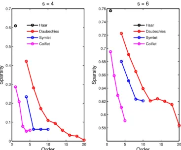
Figure 2.Sparsity of representation at scales=4 (left) ands=6 (right) for a combination of wavelet families and orders. We find that Haar provide the sparsest representation.
3.1 Choosing a wavelet
We investigate a number of wavelet families (Haar, Daubechies, Symlet, and Coiflet) in order to determine which provides the sparsest representation offV.fVis first subjected
to a wavelet transform using a chosen wavelet. At each scale
s, we remove wavelets that contribute little to fV. We set
“small” wavelet coefficients (“small” is defined as the
ra-tio|ws,i,j/wmax,s| ≤10−3, wherewmax,s is the wavelet
co-efficient on scaleswith the largest magnitude) to zero. We refer to the fraction of zero wavelet coefficients at scales
as its sparsity. Figure 2 plots the sparsity at scale s=4,6 for a large combination of wavelet families and orders. We see that the Haar wavelet (also called the Daubechies, or-der 2 wavelet) provides the sparsest representation, making it a candidate for developing a low-dimensional MsRF for ffCO2emissions. This is a consequence of the spatial
distri-bution offV – the map offV(Fig. 1b) is largely empty west
of 100◦W, which manifests itself as small coefficients for the wavelets whose support lie in that region. This favors simpler (non-smooth) and low-order wavelets.
Next we investigate the variation of the magnitude of wavelet coefficients, as a function of the type of wavelets used to modelfV. We select five wavelet types, e.g., Haar,
Daubechies, order 4 and 8, and Symlet, order 4 and 6, and perform a wavelet transform offV. At each scales, we set
1 2 3 4 5 6 −1
−0.5 0 0.5 1 1.5 2
Scale
Mean and standard deviation
Statistics of non−zero wavelet coefficients
Haar Daubechies 4 Daubechies 8 Symlet 4 Symlet 6
Figure 3. We plot the average value of the non-zero coefficients (solid lines) and their standard deviation (dashed line), at different scales s, whenfV is subjected to wavelet transforms using Haar,
Daubechies 4 and 6, and Symlet 4 and 6 wavelets. We find that while Haar may provide the sparsest representation (Fig. 2), the non-zero values tend to be large and distinct.
Daubechies, order 8, have more non-zero wavelet coeffi-cients, but with smaller wavelet coefficients. This is a con-sequence of the spatial distribution offV(Fig. 1) which has
sharp gradients, placing smooth wavelets at a disadvantage. In Fig. 3, we also see that the means and standard deviations shrink, especially after scales=3; further, the distributions of wavelet coefficients arising from the different wavelet types begin to resemble each other. This arises from the fact that there are sharp boundaries around the areas where ffCO2
emissions occur; when subjected to a wavelet transform, the region in the vicinity of a sharp boundary gives rise to large wavelet coefficients down to the finest scale. Thus the few non-zero wavelet coefficients at the finer scales assume sim-ilar values, irrespective of the wavelet type.
Finally, we check the accuracy of a Haar representation of fV at various levels of sparsity. Again, we define a “small”
wavelet as|ws,i,j/wmax,s| ≤α. We perform a wavelet
trans-form of fV using Haar wavelets and sparsify (set small
wavelets to zero) using 10−6≤α≤1. We then perform an inverse transform to reconstruct a “sparsified” fV
′ . In Fig. 4, we plot overall sparsity, reconstruction error ǫ= kfV
′
−fVk2/kfVk2and the Pearson correlation between the
true and reconstructedfV as a function ofα. We define the
Pearson correlation betweenfV
′
andfVas ρfV
′
,fV
=cov(fV,fV
′
) σf
VσfV′
,
whereσ2
fV andσ
2
fV′ are the variances of the true and
recon-structed fluxes and cov(Z1, Z2) is the covariance between
two random variablesZ1andZ2. Herek · k2denotes theℓ2
norm. We find that forα <10−2there is practically no error
10−6 10−5 10−4 10−3 10−2 10−1 100 0
0.2 0.4 0.6 0.8 1
Threshold fraction α
Sparsity & reconstruction error
Reconstruction fidelity versus sparsity
10−6 10−5 10−4 10−3 10−2 10−1 100
0 0.2 0.4 0.6 0.8 1
Pearson correlation
Sparsity
Reconstruction error Correlation
Figure 4. Variation of sparsity, reconstruction error ǫ, and the Pearson correlation between the true and reconstructed fV, i.e.,
ρ(fV,fV
′
)as a function ofα.
(as measured by these metrics) though we achieve a sparsi-fication of about 80 %. Even at a sparsity of around 90 %, the error is less that 10 %. Thus a small collection of Haar wavelets have the ability to reproducefVwith an acceptable
degree of error. This low-dimensional character of a Haar representation of fV can be invaluable in an inverse
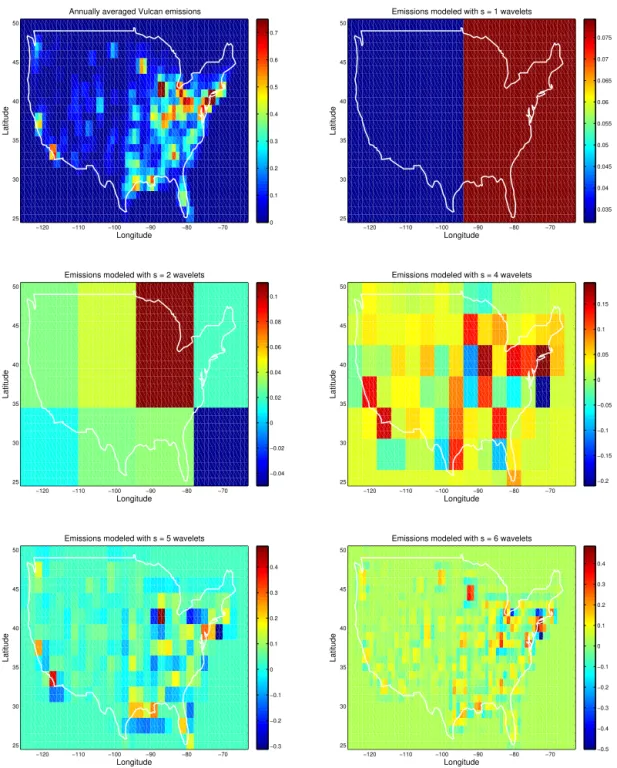
prob-lem predicated on sparse observations, and henceforth, we will proceed with Haar wavelets as the basis set of choice for representing ffCO2emissions. Figure 5 shows the
decompo-sition offVon aM=6 hierarchy of Haar wavelets.
We will use wavelets selected using the (single) nightlight and BUA maps to estimate weekly ffCO2 emissions. Our
tests above show that they model annually averaged Vulcan emissions adequately, and we assume that while emissions may wax and wane with time, their spatial distribution does not vary sufficiently to require a new wavelet selection. We base this assumption on ffCO2 emissions’ correlation with
human activities and static sources like powerplants which do not display large spatial dislocations with time. Note that the location and strengths of intense sources of ffCO2emissions,
such as powerplants, can be found at the CARMA (Carbon Monitoring for Action; website http://carma.org). Note, also, that CARMA isnotpeer-reviewed and only provides data for a limited number of years (version 3.0 has data only for 2004 and 2009).
3.2 Constructing a random field model
We seek a spatial parameterization for ffCO2emissions, of
the form
f=w′φ′+
M
X
s=1
X
i,j
ws,i,jφs,i,j, {s, i, j} ∈W(s), (3)
−120 −110 −100 −90 −80 −70 25
30 35 40 45 50
Longitude
Latitude
Annually averaged Vulcan emissions
0 0.1 0.2 0.3 0.4 0.5 0.6 0.7
−120 −110 −100 −90 −80 −70
25 30 35 40 45 50
Longitude
Latitude
Emissions modeled with s = 1 wavelets
0.035 0.04 0.045 0.05 0.055 0.06 0.065 0.07 0.075
−120 −110 −100 −90 −80 −70
25 30 35 40 45 50
Longitude
Latitude
Emissions modeled with s = 2 wavelets
−0.04 −0.02 0 0.02 0.04 0.06 0.08 0.1
−120 −110 −100 −90 −80 −70
25 30 35 40 45 50
Longitude
Latitude
Emissions modeled with s = 4 wavelets
−0.2 −0.15 −0.1 −0.05 0 0.05 0.1 0.15
−120 −110 −100 −90 −80 −70
25 30 35 40 45 50
Longitude
Latitude
Emissions modeled with s = 5 wavelets
−0.3 −0.2 −0.1 0 0.1 0.2 0.3 0.4
−120 −110 −100 −90 −80 −70
25 30 35 40 45 50
Longitude
Latitude
Emissions modeled with s = 6 wavelets
−0.5 −0.4 −0.3 −0.2 −0.1 0 0.1 0.2 0.3 0.4
Figure 5.Annually averaged Vulcan emissionsfVare modeled using Haar wavelets on scales 1, 2, 4, 5, and 6. The figure at the top (left)
plotsfV, and the rest its decomposition across wavelet scales. Note that we have displayed only the relevant part of the dyadic 2M×2Mgrid
on which wavelets are described.
easily observed proxy X of human activity (which correlates with ffCO2 emissions) to select the
com-ponents of W(s). Radiance calibrated nightlights (http://www.ngdc.noaa.gov/dmsp/download_radcal.html; Cinzano et al., 2000) have been used for constructing ffCO2 inventories (Doll et al., 2000) and are an
obvi-ous choice for X. However, nightlight radiances are also
information from IGBP (International Geosphere–Biosphere Programme, http://www.igbp.net/) land-cover map. The two choices forXwill be compared with respect to (1) sparsity, (2) the correlation betweenXandfV, and (3) the ability of W(s)to capturefV.
In Fig. 6 (top row), we plot maps of the two proxies, coars-ened to 1◦resolution. Comparing with Fig. 1 (bottom), we see that they bear a strong resemblance tofV. We subjectXto
a wavelet transform and set all wavelet coefficients|ws,i,j|< δto zero, whereδis a user-defined threshold. The bases with non-zero coefficients are selected to constituteW(s). We re-constitute a “sparsified” proxy, X(s), using just the bases in
W(s), and compute the correlation betweenX(s)andfV.
Fi-nally, we projectfV ontoW(s), obtain its “sparsified” form
fV (s)
, and compute the error ǫf = kfV (s)
−fVk2/kfVk2. In
Fig. 6 (middle row), we plot the sparsity, correlation andǫf
for various values of δ. We do so for both nightlights and BUA. For nightlights, we achieve a sparsity of around 0.75 forδ <10−2, i.e., we need to retain only a quarter of the Haar bases to represent nightlights. The nightlights so represented bear a correlation of around 0.7 withfV, and achieve an error ǫf of around 0.1. Note that this measure of error reflects the
inability of the MsRF to represent fine-scale details, and not spatially aggregated quantities, which are represented more accurately. In contrast, using BUA as a proxy, we see that while the sparsity achieved is similar, the correlation between X(s)andfVis slightly higher. The behavior ofǫf is similar,
except the error increases faster withδ, as compared to night-lights. However both nightlights and BUA maps show signif-icant correlation withfVand the sparsified set of Haar bases
that they (i.e., the proxies) provide (using δ=10−2in both the cases) allow us to construct a low-dimensional parame-terization of ffCO2emissions.
Finally, we useX(s)to create a “prior model”fpr=cX(s)
for ffCO2emissions,f.cis computed such that
Z
R
fVdA=
Z
R
fprdA= (4)
c Z
R
w′(X)φ′+X
l,i,j
w(X),s,i,jφl,i,j
!
dA, {l, i, j} ∈W(s),
where Rdenotes the lower 48 states of USA and w(X)=
{w(X),s,i,j}are coefficients from a wavelet transform ofX.
This implies that c is calculated such that both fV and fpr
provide the same value for the total emissions for the US.c
is the ratio of the aggregate total of ffCO2emissions to the
aggregate total of radiances (for the nightlights) or percent-ages of built-up areas. In Fig. 6 (bottom row), we plot the error (fpr−fV). (The Supplement contains a scatter plot of
fpr vs.fV.) We see that neither nightlights nor the BUA map
provide afprthat is an accurate representation offV, though
they share similar spatial patterns, i.e., fpr may be used to
provide a guess forfin an inverse problem, but, by itself, is a poor predictor, regardless of the proxyXused to create it.
4 Formulation of the estimation problem
In this section, we pose and solve an inverse problem to esti-mate ffCO2emissions using the MsRF developed in Sect. 3.
The method is new, and uses a sparse reconstruction method that is summarized in Sects. 4.1 and 4.2; full details are in Ray et al. (2013). The inversion technique is most relevant in situations where accurate, finely gridded ffCO2
invento-ries are unavailable, and one has to take recourse to easily observable proxies for information on the spatial pattern of ffCO2emissions.
The inverse problem is predicated on synthetic observa-tions,yobs, of CO2concentrations measured at 35 towers (a
network that existed in 2008). These are plotted as markers in Fig. 8; see Ray et al. (2013) for their precise locations and names. The measurements are related to ffCO2emissions
de-scribed on a finely gridded domain as
yobs=y+ǫ=Hf+ǫ, (5)
whereHis the transport or sensitivity matrix, obtained from a transport model, y is the CO2 concentration predicted
by the atmospheric model, which differs from its measured counterpart by an errorǫ. The ffCO2emissionsfare defined
on a grid, and are assumed to be non-zero only withinR.
The estimation of CO2fluxes, typically biospheric (Nassar
et al., 2011; Chatterjee et al., 2012; Gourdji et al., 2012), is usually posed as the minimization of an objective functionJ,
J=(yobs−Hf)TR−e1(yobs−Hf)+(f−fm)TQ−1(f−fm), (6)
wherefm are “prior” (or guessed) fluxes and R−e1 is a
di-agonal matrix containing the standard deviation of Gaussian noise used to model measurement error. The discrepancy between the “true” and prior fluxes is modeled as a multi-variate Gaussian field, whose covarianceQis calculated of-fline. In contrast, in our ffCO2inversion,fwill be modeled
using the MsRF rather than a multivariate Gaussian field. Further, the second term in Eq. (6) is omitted and the ef-fect of the “guessed” or “prior” emissionsfpr is introduced
−120 −110 −100 −90 −80 −70 25
30 35 40 45 50
Longitude
Latitude
Nightlight radiances [W/cm2 * sr * micron]
0 5 10 15 20 25
−120 −110 −100 −90 −80 −70
25 30 35 40 45 50
Longitude
Latitude
Built−up area [%]
0 2 4 6 8 10 12 14 16 18 20
10−8 10−6 10−4 10−2 100
0 0.2 0.4 0.6 0.8 1
Sparsity & reconstruction error
Wavelet coefficient magnitude threshold δ Statistics of reconstruction, for different δ
10−8 10−6 10−4 10−2 100
0 0.2 0.4 0.6 0.8 1
Pearson correlation
Sparsity Reconstruction error, εf
Correlation
10−8 10−6 10−4 10−2 100
0 0.2 0.4 0.6 0.8 1
Sparsity & reconstruction error
Wavelet coefficient magnitude threshold δ Statistics of reconstruction, for different δ
10−8 10−6 10−4 10−2 100
0 0.2 0.4 0.6 0.8 1
Pearson correlation
Sparsity Reconstruction error, εf
Correlation
−120 −110 −100 −90 −80 −70
25 30 35 40 45 50
Longitude
Latitude
Error in the reconstructed emissions [micromoles/m2/sec]
−0.8 −0.6 −0.4 −0.2 0 0.2 0.4 0.6
−120 −110 −100 −90 −80 −70
25 30 35 40 45 50
Longitude
Latitude
Error in the reconstructed emissions [micromoles/m2/sec]
−0.8 −0.6 −0.4 −0.2 0 0.2 0.4 0.6
Figure 6.Top row: maps of nightlight radiances (left) and BUA percentage (right), for the US. Middle row: the sparsity of representation, the correlation betweenXandfVand the normalized errorǫf between the Vulcan emissionsfVand the sparsified form obtained by projecting
it onX. These values are plotted for nightlights (left) and the BUA maps (right). Bottom row: plots of(fpr−fV)obtained from nightlights
(left) and BUA maps (right).
integrating the trajectories over a North American 1◦×1◦ grid as described in Lin et al. (2003). The sensitivity of the CO2 concentration at each observation location due to
the flux at each grid cell (the “footprint”) is calculated in units of ppmv µmol−1m2s (ppmv: parts per million by vol-ume). ffCO2emissions were averaged over 8-day intervals
and the sensitivity ofyto the 8 day-averaged emissions were
obtained from the 3 h sensitivities described above by sim-ply adding the 8×24/3=64 sensitivities that span the 8-day period. Thereafter, the grid cells outsideRwere removed to
obtain theHmatrix used in this study. The size of theH ma-trix is(KsNs)×(NRK), whereKs is the number of tower
covered by the lower 48 states of the US andKis the number of 8-day periods that constitute the duration over which the emissions are estimated.
4.1 Posing and solving the inverse problem
We denote the spatial distribution of emissions during an ar-bitrary 8-day periodkasfk. The 8-day period was chosen to
minimize aggregation error. We seek emissions over an en-tire year, i.e., we seek F= {fk}, k=1. . . K. We will model
emissions on the 2M×2M, M=6 mesh with wavelets:
fk=wk′φ′+ M
X
s=1
X
i,j
ws,i,j,kφs,i,j, {s, i, j} ∈W(s)
=8wk. (7)
Note that 8 comprises of only those wavelets selected using X and contained in W(s). For the entire year, the expression for emissions becomes F= {f1,f2, . . .fK} =
{8w1,8w2, . . .8wK} =e8w. Since 8wk models the
emis-sions over all grid cells, i.e., over the rectangular region given by the corners (24.5◦N, 63.5◦W) and (87.5◦N, 126.5◦W), and not justR,Fcontains emissions over the lower 48 states, as well as the region outside it (where we have assumed that the emissions are non-existent). We separate out the two fluxes by permuting the rows of8e
F=
FR
FR′
= ee8R 8R′
w,
wheree8Rand8eR′are(NRK)×(LK)and(NR′K)×(LK) matrices, respectively. Here Lis the number of wavelets in
W(s)andNR′ is the number of grid cells inR′, the region outside Rbut inside the rectangular domain. The modeled
concentrations at the measurement towers, caused by FR,
can be written asy=HFR. For arbitraryw,FR′, the emis-sions in the region outsideR, are not zero. Consequently, it
will be necessary to specify FR′=0 as a constraint in the inverse problem.
Specifying the constraintFR′ =0 directly is not very ef-ficient since it leads toNR′K constraints. In a global inver-sion, or at resolutions higher than 1◦×1◦, this could get very large. Consequently, we adapt an approach from compressive sensing to enforce this constraint approximately. Consider aMcs×(NR′K)matrixR, whose rows are direction cosines of random points on the surface ofNR′K-dimensional unit sphere. This is called a uniform spherical ensemble (Tsaig and Donoho, 2006). The projection of the emission fieldFR′ onR, i.e.,RFR′compressively samplesFR′.Mcsis the num-ber of such projections or compressive samples. Setting this projection to zero during inversion allows us to enforce zero emissions outside R. However, to do so, we add onlyMcs
constraint equations. The computational savings afforded by imposing the FR′=0 constraint in this manner is investi-gated in Ray et al. (2013).
The equivalent of Eq. (5) is written as Y=
yobs 0
≈
He8R
Re8R′
w=Gw. (8)
We incorporate the spatial patterns in X into the esti-mation procedure by using w(X) to normalize w. Other,
less effective, methods were investigated and discarded in Ray et al. (2013). We rewrite Eq. (8) as
Y≈Gdiag w(X)diag
w−(X)1
w=G′w′=
He8′R
Re8′R′
w′, (9) wherew′= {ws,i,j/(c w(X),s,i,j)},{s, i, j} ∈W(s), is the
nor-malized set of wavelet coefficients, e8′R=e8R diag(w(X))
ande8′R′=8eR′diag(w(X)).
The underdetermined system Eq. (9) is solved using opti-mization. Given the small number of towers (35) and their lo-cation (the towers were sited with biospheric fluxes in mind), it may not be possible to estimate all the elements ofw′, es-pecially those that contribute to the fine-scale details ofFR.
Further, a priori, we do not know the identity of these “un-estimatable” wavelet coefficients in w′. Consequently, we employ a sparse reconstruction method, based onℓ1
mini-mization, that identifies and estimates the elements ofw′that can be constrained byyobs, while setting the rest to zero. We cast the optimization problem as
minimize
w′∈RN kw
′k
1, subject tokY−G′w′k22< ǫ2. (10)
This is of the same form as Eq. (2) and is solved using stagewise orthogonal matching pursuit (StOMP) (Donoho et al., 2012).
4.2 Imposing non-negativity on ffCO2fluxes
Estimates of w′ calculated by StOMP do not necessarily provide non-negative estimates ofFR=e8Rw. In practice
negative ffCO2 emissions occur in only a few grid cells
and are usually small in magnitude. We devised an iterative method to impose non-negativity as a post-processing step. We present a summary here; details are in Ray et al. (2013).
We use the StOMP solution to generateF=e8w, discard FR′ and manipulate the emissionsE= {Ei}, i=1. . . NRK
inRdirectly. We start with a guessedE(= |FR|) and at the mth iteration calculate an increment1E(m−1)to the current iterateE(m−1)
yobs−HE(m−1)=1y≈H1E(m−1). (11) This is an underdetermined problem, and we seek the sparsest set of increments 1E(m−1) using StOMP. The increment is used to calculate a correction ξ = {ξi}, i=
1. . . NRK,|ξi| ≤1 and updateE(m−1) ξi=sgn
1E(mi −1)
E(mi −1) !
max 1,
1Ei(m−1)
Ei(m−1) !
, (12)
The iteration is stopped whenkyobs−HEk2/kyobsk2≤ǫ3
for a small value ofǫ3.
5 Numerical tests
Numerical tests are performed for the domain between the corners 24.5◦N, 63.5◦W and 87.5◦N, 126.5◦W. It is dis-cretized by a 2M×2M,M=6 mesh, with 4096 grid cells. Of these,NR=816 cells lie insideR, while the rest,NR′= 4096−816=3280 lie outside inR′. We estimate emissions
overk=1. . . K, K=45, i.e., for 45×8=360 days (approx-imately a year). We generate synthetic observationsyobs us-ing the ffCO2emissions in Vulcan, which provides them only
inR. Hourly Vulcan fluxes are coarsened from 0.1◦ resolu-tion to 1◦, and averaged to 8-day periods. These fluxes are multiplied byHto obtain ffCO2concentrations at theNs=
35 measurement towers. Observations are available every 3 h and span a full year, i.e., we collectKs=24/3×360=2880
observations per tower. A measurement errorǫ∼N (0, σ2)is added to the concentrations to obtainyobs, as used in Eq. (8). The same σ is used for all towers and is set to a very low value of 0.1 ppmv. Although such a value is unrealistically small for real-data inversions, it is used here to isolate the impact of the proposed parameterization and inversion ap-proach.
We solve Eq. (10) and enforce non-negativity on FR to
obtainE. The coefficientsw(X)used in Eq. (9) are obtained
from a wavelet decomposition of fpr based on nightlights
(Sect. 3). The constantcin Eq. (4) is obtained by using fluxes from the Emission Database for Global Atmospheric Re-search (EDGAR, http://edgar.jrc.ec.europa.eu; Olivier et al., 2005) for 2005, i.e., instead of using emissions from Vul-can to calculatefV, we use EDGAR. EDGAR emissions
ag-gregated over R are 7.1 % higher than fV, resulting in a
correspondingly higher c. The RMSE between the two is 0.035 µmoles m−2s−1 of C and the Pearson correlation co-efficient is 0.726. Also, sincecis an aggregate total overR,
it reflects the I.E.A country total. The following parameters are used in the inversion process (Sect. 4.2):ǫ2=10−5, ǫ3=
5.0×10⁻⁴, Mcs=13 500, i.e., 300 compressive samples for
each 8-day period. The numerical values ofǫ2 andǫ3were
set by reducing them till the solutionw′became insensitive to them. The setting forMcs is more involved and is described
in Ray et al. (2013). The initial guess for w′ in Eq. (10) is zero.
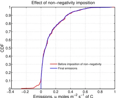
In Fig. 7 we plot the cumulative distribution function (CDF) of ffCO2emissions before and after the enforcement
of non-negativity. We see the existence of a few grid cells with negative fluxes, but their magnitudes are not very large. Thus the sparse reconstruction scheme provides a good start-ing guess for the imposition of non-negativity via the iterative method described in Sect. 4. In Fig. 8, we plot the true and reconstructed emissions for the 33rd 8-day period (k=33). We also plot the estimation error(Ek−fV,k), averaged over
−0.40 −0.2 0 0.2 0.4 0.6 0.8 1 0.1
0.2 0.3 0.4 0.5 0.6 0.7 0.8 0.9 1
Emissions, µ moles m−2 s−1 of C
CDF
Effect of non−negativity imposition
Before imposition of non−negativity Final emissions
Figure 7.CDF of emissions inR, before and after the imposition of
non-negativity, as described in Sect. 4. We see that the CDF of the emissions without non-negativity imposed contains a few grid cells with negative fluxes; further, the magnitude of the negative emis-sions is small. Thus the spatial parameterization, with sparse recon-struction, provides a good approximation of the final, non-negative emissions.
the 32-day period 33≤k≤36. We see that the reconstruc-tion in the NE quadrant is qualitatively similar to the true emissions. In contrast, the reconstruction on the west coast contains significant inaccuracies. For example, we see that the Los Angeles–San Diego region (southwest quadrant) is estimated incorrectly. The estimated emissions in the center of the country (Continental Divide and Great Plains, in the western quadrants) show similar errors, as well as far more structure than the true ffCO2 emissions. The region around
the Gulf of Mexico is also not well estimated. The quality of the reconstruction in the various regions correlate with the density of observations towers, though the wind fields also play an important part. In the regions where the observa-tions are not very informative, the impact of normalization byfpr is clear as some of its structure is retained in the
es-timated emissions. These errors are almost entirely at fine spatial scales.
In Fig. 9 (top) we plot a time-series of errors defined as a percentage of total, country-level Vulcan emissions. Per-cent errors in reconstructed emissions andfpr are calculated
−120 −110 −100 −90 −80 −70 25
30 35 40 45 50
Longitude
Latitude
True emissions in 8−day period 33 [micromoles m−2 s−1]
0 0.1 0.2 0.3 0.4 0.5 0.6 0.7
−120 −110 −100 −90 −80 −70
25 30 35 40 45 50
Longitude
Latitude
Estimated emissions in 8−day period 33 [micromoles m−2 s−1]
0 0.1 0.2 0.3 0.4 0.5 0.6 0.7
−120 −110 −100 −90 −80 −70
25 30 35 40 45 50
Longitude
Latitude
Estimation error; k = 33 ... 36
−0.3 −0.2 −0.1 0 0.1 0.2 0.3 0.4 0.5 0.6 0.7
Figure 8.Reconstruction of the ffCO2emissions from the 35
tow-ers (plotted as diamonds). The true emissions are on top and the reconstructions in the middle. The figures represent emissions for k=33 (end of August). At the bottom, we plot the estimation error, (Ek−fV ,k), averaged over 33≤k≤36. We see that the large-scale
structure of the emissions have been captured. The west coast of the US has few towers near heavily populated regions and thus is not very well estimated. On the other hand, due to the higher density of towers in the northeast, the true and estimated emissions are qual-itatively similar and estimation error are low. Emissions have units of µmol m−2s−1of C (not CO2).
Errork(%)=
100
K K
X
k=1
Ek−EV,k EV,k
,
whereEk=
Z
R
EkdA (13)
andEV,k=
Z
R
fV,kdA,
Errorpr,k(%)=
100
K K
X
k=1
Epr−EV,k
EV,k ,
whereEpr=
Z
R
fprdA.
Here,fV,k are Vulcan emissions averaged over thekth
8-day period andEk are the non-negativity enforced emission
estimates in the same time period. A positive error denotes an overestimation by the inverse problem. We see 25 % errors infpr. The large error is a consequence not only of the
dis-agreement between EDGAR (from 2005) and Vulcan (from 2002), but also the manner in which they account for emis-sions. As can be seen, assimilation ofyobsreduces the error significantly vis-à-visfpr. The least accurate reconstructions
are during spring (k=10–15). In order to check the accuracy of the spatial distribution ofEk, we calculate the Pearson
cor-relationsρ(Ek,fV,k)andρ(fpr,fV,k). We see that data
assim-ilation results in a clear increase in the correlation. When the emissions are aggregated/averaged over 32-day periods, the correlation increases to about 0.85, whereas the “prior” cor-relation was around 0.7. Thus the ffCO2emissions obtained
using a nightlight proxy are substantially improved by the in-corporation ofyobs. Only about half the wavelet coefficients could be estimated; the rest were set to zero by the sparse reconstruction technique (Ray et al., 2013).
We next investigate the effect of using BUA maps, in-stead of nightlights, as the proxy. Changing the proxy results in a different set of wavelets being chosen (nightlights re-sulted in aW(s) of 1031 wavelets; the corresponding num-ber for BUA was 1049); further, one was not a strict sub-set of the other. It also results in a different normalization in Eq. (9). The inversion was performed in a manner iden-tical to that adopted for the nightlight proxy. In Fig. 9 (top) we see that the ffCO2emissions developed using nightlights
0 10 20 30 40 50 0
5 10 15 20 25 30 35
Percent error in total emissions
8−day period
% error in total emissions
Built−up area map reconstruction Nightlight reconstruction Built−up area map prior Nightlight prior
0 10 20 30 40 50
0.2 0.3 0.4 0.5 0.6 0.7 0.8 0.9 1
Correlation between reconstructed and true emissions
8−day period
Correlation
C(Ek, fV,k)), 8−day resolution; from built−up area maps C(E
k, fV,k), 32−day resolution; from built−up area maps
C(E
k, fV,k), 8−day resolution; from nightlights
C(E
k, fV,k), 32−day resolution; from nightlights
C(f
pr, fV,k); from built−up area maps
C(f
pr, fV,k); from nightlights
Figure 9.Comparison of reconstruction error and correlations. Top: we plot the error between the reconstructed and true (Vulcan) emis-sions in black (using nightlights as priors) and in blue (using BUA priors). We plot the error betweenfpr and Vulcan emissions using
dashed lines – black for nightlights and blue for BUA. We see that assimilation ofyobsleads to significantly improved accuracy vis-à-visfpr. Bottom: we plot the accuracy of the spatial distribution of
the reconstructed emissions. The Pearson correlationsρ(Ek,fV,k)
andρ(fpr,fV,k)show that incorporatingyobsmarginally improves
the spatial agreement of estimated emissions vs. the true one when using nightlights, though the results are less clear for BUA priors. If the emissions are averaged over 32-day periods, rather than 8-day periods, the correlation with true (Vulcan) emissions rises to around 0.85, irrespective of the prior used.
emissions from Vulcan are different for nightlights and BUA reflecting the distinct spatial difference between them as seen in Fig. 6. This results in the difference between the two dashed lines. Averaging over 32-day intervals improves the correlation and makes them almost indistinguishable from those obtained using nightlights.
0 10 20 30 40 50
−80 −60 −40 −20 0 20 40 60 80
8−day periods
Emission error %
Error in reconstructed emissions in each quadrant
NW; bulit−up area NE; bulit−up area NW; nightlights NE; nightlights
0 10 20 30 40 50
−0.2 −0.1 0 0.1 0.2 0.3 0.4 0.5 0.6 0.7 0.8
8−day periods
Pearson corr coefficient
Correlation between reconstructed & true emissions
NW; bulit−up area NE; bulit−up area NW; nightlights NE; nightlights
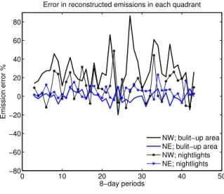
Figure 10.Top: emission reconstruction error in the NE (blue) and NW (black) quadrants, when performed with BUA (line) and night-lights (symbols) as proxies. We see that the NW quadrant is very badly constrained and the BUA-based estimates have very large er-rors. The errors in the NE quadrant are far smaller and very similar when generated using the competing proxies. Bottom: the compari-son of correlations between true and reconstructed emissions shows similar trends.
In Fig. 10 we investigate the differences between the nightlight- and BUA-based reconstructions at the quadrant level. We see in Fig. 10 (top) that the difference between nightlight- and BUA-based reconstruction errors in the NE quadrant are smaller than those for the NW quadrant. Thus, while thefpr from nightlights and BUA are quite different
(see the last row of Fig. 6), the estimated emissions are well informed by yobs in the NE quadrant and the impact of the proxies is small. This is not the case for the NW quadrant, where the reconstruction based on BUA is clearly much worse than the nightlight-based reconstruction. This is not surprising given the paucity of towers there (see Fig. 8), which increases the impact of fpr. In Fig. 10 (bottom) we
−120 −110 −100 −90 −80 −70 25
30 35 40 45 50
Longitude
Latitude
Difference in estimates in period 34 [micromoles m−2 s−1]
−0.8 −0.6 −0.4 −0.2 0 0.2 0.4 0.6 0.8 1 1.2
0 10 20 30 40 50 60 70
−0.2 0 0.2 0.4 0.6 0.8 1 1.2
Observation number
Concentration, ppmv of C
Observed and predicted CO
2 concentrations
AMT; observed AMT; predicted FRD; observed FRD; predicted NGB; observed NGB; predicted
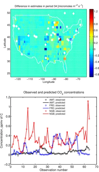
Figure 11.Top: comparison of emission estimates developed using
fprconstructed from nightlight radiances and BUA maps. We plot
the difference between the two estimates. We see that differences are not localized in any one area. Bottom: prediction of ffCO2 con-centrations at three measurement locations, using the true (Vulcan; plotted with symbols) and reconstructed emissions (blue lines) over an 8-day period (Period no. 31). Observations occur every 3 h. We see that the concentrations are accurately reproduced by the esti-mated emissions.
in the NE and NW quadrants. We see that there is little to choose between the correlations generated using nightlight-vs. the BUA-based emission estimates. Again, due to the larger density of towers in the NE, the correlations are higher there. Thus, while Fig. 6 (middle row) showed that BUA had a slightly better correlation with true (Vulcan) emissions, its larger errors, as seen in Fig. 6 (bottom row) lead to a less accurate reconstruction. This result is also a testament to the inadequacy of yobsover the whole country for constraining ffCO2emissions; had there been sufficient data to informE,
the impact offprwould have been minimal.
Next, in Fig. 11 (top) we compare the estimated emis-sions for the 34th 8-day period developed from the two competing prior models. We plot the difference between the
two estimates; it shows differences spread over a large area, though their magnitudes are not very big. Thus the “prior” model has a measurable impact on the spatial distribution of the emissions. In Fig. 11 (bottom) we plot y predicted by the reconstructed emissions (from nightlights as priors) at 3 towers. The towers were chosen to represent the range of the ffCO2 signal strengths encountered in our test cases.
We see that the ffCO2 concentrations are well reproduced
by the estimated emissions. Further, note that the measure-ment noise (σ=0.1 ppmv) is relatively large compared to some of the observations. Thus, the lack of fidelity at the smaller scales (seen in Fig. 8) does not substantially impact the measurements. This is due to the weak strengths of the er-roneous emission sources (while a few may be intense, they are present only over a small area) and their distance from the towers.
6 Discussion
The numerical results in Sect. 5 show that the MsRF and sparse reconstruction techniques can solve the inverse prob-lem as formulated in Sect. 4, conditioned on limited mea-surements of ffCO2concentrations. The solution reproduces
large-scale spatial patterns of the true flux field, and some of the finer ones. The rough spatial nature of the emission field is preserved in the estimates. Furthermore, the method is insensitive to underreporting of ffCO2emissions by
coun-tries which are used to construct inventories such as EDGAR. Inventories are used only to calculatecin Eq. (4) which ap-pears as a normalization constant in Eq. (9). The accuracy of the estimates (the constraint||Y−G′w′||22< ǫ2in Eq. (10))
is unaffected by the value ofc. The chief source of errors in the estimates is the paucity of observations sensitive to fossil-fuel-emitting regions. Regions with low tower density, e.g., the western quadrants in Fig. 8, have large errors due to the faint ffCO2 signal at existing observational sites. One
limi-tation of the deterministic estimation method presented here is that it does not provide any measure of the uncertainty in the estimates. The numerical parametersǫ2,ǫ3andMcs are
not significant sources of uncertainty since they were set at values where the solution of the inverse problem became in-sensitive to them.
Given our focus on the algorithmic issues in the esti-mation of ffCO2 emissions under realistic conditions, the
inverse problem that we constructed is idealized and em-bodies a number of simplifications. We have used a sen-sor network (that existed in 2008) that was sited with an eye towards estimating biospheric CO2fluxes. This network
is therefore not optimized for constraining ffCO2 emission
sources, leading to a faint ffCO2 signal (<2 ppmv). This
made the use of a small model–data mismatch error neces-sary for the synthetic-data experiments presented here (σ=
the availability of observations that isolate the ffCO2
sig-nal, which would either require observations of a ffCO2
ns-specific tracer, or the pre-subtraction of the influence of bio-spheric fluxes from observations. Some of the other simplifi-cations used in the setup, on the other hand, are common to synthetic-data inversion experiments focusing on biospheric fluxes and reported elsewhere, e.g., Gourdji et al. (2010). For example, we have ignored emissions outside R; in a
real-istic ffCO2estimation problem, emissions outsideRwould
have to be modeled as boundary conditions to the examined domain, as is done for regional biospheric inversion studies. Furthermore, we have also assumed a constant data–model mismatch (σ) across all sensors, and site- and seasonally varying model–data mismatch statistics would be required when real data are used.
The use of proxies to construct the MsRF for ffCO2
emis-sions can be a source of estimation errors and consequently, in Sects. 3 and 5, we investigated nightlights and BUA maps to explore the impact of using such proxies for sub-selecting the wavelets to be used in the inversion. Errors in the prox-ies themselves (i.e. inaccuracprox-ies in the nightlights and BUA data themselves) are unlikely to be a large source of estima-tion errors in the inversion, as these proxies are used only to select wavelets, whereas the wavelet coefficients are ob-tained in the inversion step. Rather, inversion errors can stem from the fact that nightlights correlate with energy consump-tion and not energy producconsump-tion. This can lead to two types of errors: (1) when a fine-scale wavelet covering a region with a strong ffCO2 source and little human habitation is
omit-ted from the MsRF and (2) when we choose a “superfluous” fine-scale wavelet in a region with much human activity and little emission. An example of the first type of error is large powerplants, which are usually sited far from densely popu-lated areas. In such a case, the point-source is modeled by the coarse-scale wavelet that covers the area in question, leading to a “smeared” reconstruction. Such large point-sources of ffCO2 emissions could instead be obtained from databases
such as CARMA and incorporated directly into the inver-sion. Alternatively, one could augment the wavelets in the MsRF with those chosen using a second proxy, e.g., thermal images, where large emitters of heat can be easily detected. The second type of error, that of the “superfluous” wavelet, is rectified when it is simply removed by the sparse reconstruc-tion scheme in the inversion step. An excepreconstruc-tion can occur if the superfluous wavelet contains a measurement tower in its supportandis far from all other towers. Since measurement towers are very sensitive to fluxes in their vicinity (Gerbig et al., 2009), it could lead to the estimation of a spurious emission source.
ffCO2emissions, averaged over 8-day intervals and
pred-icated on 3-hourly measurements, were estimated as inde-pendent variables, i.e., without imposing a temporal correla-tion or modeling their temporal evolucorrela-tion in any way. The reason is as follows. Estimation of ffCO2 emissions over
a 8-day interval requires the calculation of 1031 wavelet
coefficients (when using the nightlights-derived MsRF) from 35×8×8=2240 measurements. This is not an underdeter-mined problem, even though a sparse reconstruction method was required to remove fine-scale structures (wavelets) in the emission field that did not affect the measurements. We were able to constrain the coefficients of the remaining wavelets without imposing a temporal correlation structure. Such cor-relations could be used if ffCO2fluxes were to be estimated
at finer temporal resolution.
The spatial parameterization and the sparse reconstruction method can also be used in observation system simulation experiments (OSSEs) to inform the design of measurement networks targeted for ffCO2emissions. The approach can be
used to decide locations of towers, the frequency at which ffCO2measurements are to be made, and the fidelity required
in measurements and the transport model. The trade-offs and costs of various ffCO2measurement technologies can also be
studied in such a setting. In addition, OSSEs can reveal the importance of a more accurate MsRF, e.g., one augmented using thermal imagery, vs. the errors introduced in the esti-mates due to limited measurements.
7 Conclusions
We have devised a multiresolution parametrization (also known as a multiscale random field or MsRF model) for modeling ffCO2emissions at 1◦resolution. The MsRF
mod-els emissions in the lower 48 states of the US and is designed for use in atmospheric inversions. The parameterization em-ploys Haar wavelets which provide a sparser representation than other smoother wavelets with wider support. This is the first “abstract” parameterization, i.e., a RF model for spa-tially resolved ffCO2emissions.
The dimensionality of the MsRF was reduced by judi-ciously selecting its component Haar wavelets using proxies of human activity, and therefore indicative of ffCO2
emis-sions. We developed two MsRFs based on images of lights at night and maps of built-up areas. The former had a slightly lower dimensionality but was not a strict subset of the latter. The MsRF models were also used to develop two approxi-mate emission models that differed in their fine spatial de-tails.
The MsRF model was tested in a synthetic-data inversion. Time-dependent ffCO2emissions, averaged over 8-day
pe-riods, were estimated for a 360-day period from measure-ments of ffCO2 concentrations at 35 towers. These
obser-vations were sufficient only for estimating about half the wavelets retained in the MsRF model. We used a sparse re-construction technique, namely Stagewise Matching Orthog-onal Pursuit (StOMP), to identify and estimate wavelet coef-ficients in MsRF that could be informed by the available data. The StOMP estimates were not necessarily non-negative (as ffCO2 emissions are required to be) and we devised an