www.atmos-chem-phys.net/14/7273/2014/ doi:10.5194/acp-14-7273-2014
© Author(s) 2014. CC Attribution 3.0 License.
Simulating the integrated summertime
1
14
CO
2
signature from
anthropogenic emissions over Western Europe
D. Bozhinova1, M. K. van der Molen1, I. R. van der Velde1, M. C. Krol1,2, S. van der Laan3, H. A. J. Meijer3, and
W. Peters1
1Meteorology and Air Quality Group, Wageningen University, the Netherlands 2Institute for Marine and Atmospheric Research Utrecht, Utrecht, the Netherlands 3Centre for Isotope Research, University of Groningen, Groningen, the Netherlands
Correspondence to:D. Bozhinova ([email protected])
Received: 7 November 2013 – Published in Atmos. Chem. Phys. Discuss.: 21 November 2013 Revised: 30 April 2014 – Accepted: 27 May 2014 – Published: 17 July 2014
Abstract. Radiocarbon dioxide (14CO2, reported in
114CO2) can be used to determine the fossil fuel CO2
addition to the atmosphere, since fossil fuel CO2no longer
contains any 14C. After the release of CO
2 at the source,
atmospheric transport causes dilution of strong local signals into the background and detectable gradients of 114CO2
only remain in areas with high fossil fuel emissions. This fossil fuel signal can moreover be partially masked by the enriching effect that anthropogenic emissions of 14CO2
from the nuclear industry have on the atmospheric114CO2
signature. In this paper, we investigate the regional gradients in 14CO2 over the European continent and quantify the
effect of the emissions from nuclear industry. We simulate the emissions and transport of fossil fuel CO2 and nuclear 14CO
2 for Western Europe using the Weather Research
and Forecast model (WRF-Chem) for a period covering 6 summer months in 2008. We evaluate the expected CO2
gradients and the resulting 114CO2in simulated integrated
air samples over this period, as well as in simulated plant samples.
We find that the average gradients of fossil fuel CO2 in
the lower 1200 m of the atmosphere are close to 15 ppm at a 12 km×12 km horizontal resolution. The nuclear influ-ence on114CO2signatures varies considerably over the
do-main and for large areas in France and the UK it can range from 20 to more than 500 % of the influence of fossil fuel emissions. Our simulations suggest that the resulting gradi-ents in114CO2are well captured in plant samples, but due
to their time-varying uptake of CO2, their signature can be
different with over 3 ‰ from the atmospheric samples in
some regions. We conclude that the framework presented will be well-suited for the interpretation of actual air and plant14CO2samples.
1 Introduction
The magnitude of anthropogenic fossil fuel CO2emissions
Several atmospheric monitoring strategies for fossil fuel emissions have been applied in recent years. Most of these use spatiotemporal variations in CO2mole fractions (Koffi
et al., 2013), often augmented with various other energy re-lated gases such as CO (Levin and Karstens, 2007), NOx
(Lopez et al., 2013), or SF6 (Turnbull et al., 2006). An
ad-vantage of these other gases is that they can be measured continuously and relatively cheaply with commercially avail-able analyzers, of which many have already been deployed. However, one of the disadvantages lies in attribution, as each process induces its own typical ratio of these gases to the atmosphere. An example is the much higher CO / CO2
ra-tio produced by traffic emissions than by power plants. An-other disadvantage is that not all of these trace gases are di-rect proxies for fossil fuel CO2release as some have totally
independent, but co-located sources with the sources of an-thropogenic CO2emissions. This is in large contrast with the
one tracer that is generally considered the “gold standard” for fossil fuel related CO2detection: radiocarbon dioxide or 14CO
2(Kuc et al., 2003; Levin et al., 2003, 2008; Levin and
Karstens, 2007; Levin and Rödenbeck, 2008; Turnbull et al., 2006; Djuricin et al., 2010; Miller et al., 2012), reported usu-ally as114CO2(Stuiver and Polach, 1977; Mook and van der
Plicht, 1999).
Radiocarbon derives its strength for fossil fuel monitoring from the absence of any14C in carbon that is much older than
the typical half-life time of the radiocarbon−5700±30 years (Roberts and Southon, 2007). This typically applies only to carbon in fossil reservoirs, as other carbon reservoirs are con-tinuously supplied with fresh14C from exchange with the at-mosphere where 14CO2is produced in the stratosphere and
upper troposphere (Libby, 1946; Anderson et al., 1947). In the natural carbon balance this14C would cycle through the atmospheric, biospheric, and oceanic reservoir until it de-cays. But very large anthropogenic disturbances on this nat-ural cycle come specifically from (a) large scale burning of very old and14C depleted carbon from fossil reservoirs, the “Suess effect” (Suess, 1955; Levin et al., 1980), and (b) pro-duction of highly enriched14C in CO2such as from nuclear
bomb tests (Nydal, 1968), or some methods of nuclear power production (McCartney et al., 1988a, b). Samples of14CO
2
taken from the atmosphere, but also from the oceans and bio-sphere that exchange with it, consistently show their domi-nant influence on the14CO2budget of the past decades (e.g.:
Levin et al., 1989, 2010; Meijer et al., 1996; Nydal and Gisle-foss, 1996; Levin and Hesshaimer, 2000; Randerson et al., 2002; Naegler and Levin, 2006; Graven et al., 2012a, b).
Monitoring of atmospheric14CO2is done through several
methods. One commonly applied approach is by absorption of gaseous CO2into a sodium hydroxide solution from which
the carbon content is extracted for14C / C analysis either by radioactive decay counters, or converted into a graphite target for analysis by accelerator mass spectrometry. The air flow-ing into the solution typically integrates the absorbed CO2
with sampling time of days, weeks, or even longer periods.
While there is a new technique, which uses integrated flask sampling (Turnbull et al., 2012), the other method generally used is to collect an air sample in a flask, which is filled within less than a minute and thus representative of a much smaller atmospheric time-window. Compared to these, at the other end of the time spectrum is the use of plants to sample
14C / C ratios in the atmosphere through their photosynthetic
fixation of atmospheric CO2. Depending on the species these
integrate over sampling windows of a full growing season (annual crops, fruits – Shibata et al., 2005; Hsueh et al., 2007; Palstra et al., 2008; Riley et al., 2008; Wang et al., 2013) or longer (trees, tree-rings – Suess, 1955; Stuiver and Quay, 1981; Wang et al., 2012).
An effective monitoring strategy for fossil fuel emissions is likely to take advantage of all methods available to collect
14C samples, and combine these with high resolution
mon-itoring of related gases (e.g. CO, SF6). Levin and Karstens
(2007), van der Laan et al. (2010) and Vogel et al. (2010) al-ready demonstrated the viability of a monitoring method in which observed CO / CO2 ratios are periodically calibrated
with14CO2to estimate fossil fuel emissions at high temporal
resolutions. More recently, this strategy was also employed by Lopez et al. (2013), where additionally the CO2/ NOx
ra-tios were used to estimate fossil fuel derived CO2from
con-tinuous CO and NOx observations in Paris. Turnbull et al.
(2011) showed for the city of Sacramento, that using a com-bination of114CO2 and CO observations can reveal
struc-tural detail in CO2 from fossil fuel and biospheric sources
that cannot be obtained by CO2measurements alone. Van der
Laan et al. (2010) and recently Vogel et al. (2013) showed that the agreement between modeled fossil fuel CO2
esti-mates and observations of14C-corrected CO can be further improved by including222Rn as a tracer for the vertical mix-ing. Finally, Hsueh et al. (2007) and Riley et al. (2008) used
14C / C ratios in corn leaves and C3 grasses to reveal
fos-sil fuel emission patterns on city, state, and national scales. Given so many different methods to use14C in monitoring strategies, its increasing accuracy, reduction in required sam-ple size, and decreasing costs, it is likely that this tracer will play a more important role in the future of the carbon observ-ing network.
The quantitative estimation of fossil fuel emissions from all of the14C-based monitoring strategies above requires dif-ferent methods and emphasizes difdif-ferent terms in the14CO2
strongly on our ability to capture these diverse processes on diverse scales.
In this work, we present a newly-built framework designed to interpret14CO2from different types of samples and from
different monitoring strategies. The framework includes at-mospheric transport of surface emissions of total CO2 and 14CO
2on hourly scales on a model grid of a few kilometers,
but integrates signals up to seasonal time scales and even down into the leaves of growing crops (maize and wheat). Both regional transport and plant growth are based on me-teorological drivers that are kept consistent with large-scale weather reanalyses. In addition to fossil fuel signals in the atmosphere and in plants, we simulate the spread of nuclear derived14C release from major reprocessing plants and from operational nuclear power production plants across Europe based on work of Graven and Gruber (2011). We applied our framework to the European domain for the summer of 2008. After explaining the components of the framework (Sect. 2) we will demonstrate its application (Sect. 3.1), as-sess the fossil and nuclear derived14C gradients across Eu-rope (Sect. 3.2), and simulate the signal that will be recorded into annual crops growing across the domain (Sect. 3.3). We will evaluate its potential benefits compared to simpler but less realistic fossil fuel estimation methods from integrated samples alone (Sect. 3.4). We will conclude with a discus-sion (Sect. 4) of the application of this framework to actual measurements and recommendations for future studies.
2 Methods
2.1 The regional atmospheric CO2and114CO2budget
The regional CO2 mole fractions and 114CO2 signature
of the atmosphere observed at a particular location are described in Eqs. (1) and (2), following the methodol-ogy used by Levin et al. (2003), Turnbull et al. (2006), Hsueh et al. (2007), Palstra et al. (2008) and described thor-oughly in Turnbull et al. (2009b). Here the1xand CO2x(or 14CO
2x) indicate the114CO2signature of CO2(or 14CO2)
mole fractions of particular origin, expressed in the index as follows: obs – observed at location, bg – background, ff – fossil fuels, p – photosynthetic uptake, r – ecosystem respi-ration, o – ocean, n – nuclear and s – stratospheric.
CO2obs=CO2bg+CO2ff+CO2p+CO2r
+CO2o+CO2s (1)
1obsCO2obs=1bgCO2bg+1ffCO2ff+1pCO2p +1rCO2r+1oCO2o
+1n14CO2n+1sCO2s (2)
Several of the terms in both equations can be omitted or transformed in our study, as described next.
We set1p=1bgsimilar to the approach in Turnbull et al.
(2006) as the calculation of114CO2accounts for changes in
the signature of the photosynthesized CO2flux due to
frac-tionation. The atmosphere-ocean exchange in the northern Atlantic makes the region generally a sink of carbon (Watson et al., 2009), but we assume that its transport to our domain is uniform and captured by the inflow of background air and thus also carries the signature1bg. For the ecosystem
respi-ration and ocean exchange the terms1rand1ocan be also
written as1bg+1disbioand1bg+1disocean, where the
disequi-librium terms (1dis) describe the difference between the sig-nature of the carbon in the particular reservoir and the cur-rent atmospheric background. These differences arise from the past enrichment of the atmosphere with14CO2from the
atmospheric nuclear bomb tests since the 1960s. In the fol-lowing decades this enrichment was incorporated into the different carbon reservoirs (Levin and Kromer, 1997; Levin and Hesshaimer, 2000) and currently these terms are of dom-inant importance only in particular regions of the globe. For our domain both terms are considered of much smaller influ-ence than the dominant effect of the fossil fuels and are con-sequently omitted (Levin and Karstens, 2007; Hsueh et al., 2007; Palstra et al., 2008; Turnbull et al., 2009b; Naegler and Levin, 2009a, b; Levin et al., 2010). Because we currently do not correct for this, the omission of the biospheric disequilib-rium in the region and period of our study will likely result in a small bias in our results, as our atmosphere will be less en-riched during the period of peak biospheric activity. For the northern hemisphere Turnbull et al. (2006) estimates an over-estimation of fossil fuel CO2by 0.2–0.5 ppm or up to 1.3 ‰
enrichment in114CO2due to this lack of disequilibrium
in-fluence, while Levin et al. (2008) evaluates this influence on the observational sites in Germany to be within 0.2 ppm or about 0.5 ‰ enrichment. The intrusion of14CO2-enriched
stratospheric air can be of importance for observations in the upper troposphere or higher, however in our case this term can be considered as part of the background, as the strato-spheric14CO
2is already well mixed by the time it reaches
the lower troposphere.
Most studies ignore the effects of anthropogenic nuclear production of14CO2 on the atmospheric114CO2since on
the global scale this production averages to the smallest con-tribution, compared to the other terms (Turnbull et al., 2009a) and few try to quantify and correct for it in observations taken nearby nuclear power plants (Levin et al., 2003). However, Graven and Gruber (2011) showed that the regional influence of a dense nuclear power plant network cannot be ignored. They estimated the potential bias in the recalculation of fossil fuel CO2due to nuclear power plant production is on average
Sellafield, United Kingdom), which generally have higher than average emissions of14CO2(McCartney et al., 1988a).
Particularly the site of La Hague is estimated to be the largest current point-source of14CO2emissions in the world, in
re-cent years accounting for more than 10 % of the global bud-get of nuclear produced14CO2(Graven and Gruber, 2011).
The magnitude of this source and its spatial location close to the major fossil fuel emitters in Europe pose a challenge in estimating the uncertainty with which the method of recalcu-lating fossil fuel CO2can be applied in the region.
All these considerations allow us to simplify Eqs. (1) and (2) to Eqs. (3) and (4).
CO2obs=CO2bg+CO2ff+CO2p+CO2r (3)
1obsCO2obs=1bg(CO2bg+CO2p+CO2r)
+1ffCO2ff+114n CO2n (4)
The instantaneous 114CO2 signature of the atmosphere is
calculated using Eq. (4), using the specific signatures for var-ious sources of CO2(various1terms) as listed below:
1. Fossil fuels are entirely devoid of14CO2and their1ff= −1000 ‰.
2. The nuclear emissions are of pure14CO2and in this
for-mulation1nis the114CO2signature that a pure14CO2
sample would have. We calculate it using the activity of pure14CO2sample in the formulation of114CO2as
follows:
As=λ·Na/m14C, (5)
whereNa=6.022×10²³mol−1 is the Avogadro
con-stant, λ=3.8534×10⁻¹²Bq is the decay rate of 14C andm14C=14.0 g mol−1is the molar mass of the iso-tope. In a sample of a pure14CO2there is no
fractiona-tion and the calculafractiona-tion of114CO2(Stuiver and Polach,
1977; Mook and van der Plicht, 1999) can be simplified to the ratio between the activity of the sample and activ-ity of the referenced standard AABS=0.226 Bq g C−1
(Mook and van der Plicht, 1999):
1n=As/AABS·1000[‰] (6)
The resulting1n≈0.7×10¹⁵[‰] is much higher than
any of the other 1signatures, but this is balanced by the concentrations of the14CO2, which are only a very
small fraction (∼10−12) of the observed CO
2
concen-trations.
3. Finally, we use1bg from monthly observed 114CO2
at the high alpine station Jungfraujoch (3580 m a.s.l., Switzerland) (Levin et al., 2010), which is consid-ered representative for European114CO2background.
These are shown in red on Fig. 3a.
We note that the choice of background can be crucial for the estimation of1obs and consequently for the
recalcula-tion of CO2ff. Local influences captured in the background
might modify the seasonality of the derived 1obs and
re-sult in biases when applied to observations from other lo-cations. These influences include local fossil fuel or nuclear signals, biospheric enrichment or modified vertical mixing during parts of the year (Turnbull et al., 2009b).
The transport and resulting spatiotemporal gradients in to-tal CO2 and14CO2over Europe are simulated with
WRF-CHEM model, described next.
2.2 WRF-CHEM
For our simulation with WRF-Chem (version 3.2.1) (Ska-marock et al., 2008) we use meteorological fields from the National Centers for Environmental Prediction Final (FNL) Operational Global Analyses (NCEP, US National Centers for Environmental Prediction, 2011) at 1◦×1◦for lateral me-teorological boundary conditions, which are updated every 6 h. We model the atmospheric transport and weather for the period between April and September 2008 including. We use three domains with horizontal resolution of 36, 12 and 4 km and, respectively, 60×62, 109×100 and 91×109 grid points, centered over Western Europe and the Netherlands, as shown in Fig. 1. Our vertical resolution includes 27 pressure levels, 18 of which are in the lower 2 km of the troposphere, and the time step used is 180 s in the outer domain. Important physics schemes used are the Mellor-Yamada Nakanishi and Niino (MYNN2.5) boundary layer scheme (Nakanishi and Niino, 2006), the Rapid Radiation Transfer Model (RRTM) as our longwave radiation scheme (Mlawer et al., 1997), and the Dudhia shortwave radiation scheme (Dudhia, 1989). We use the Unified Noah Land-Surface Model (Ek et al., 2003) as our surface physics scheme and additionally use time-varying surface conditions, which we update every 6 h.
We use separate passive tracers for the different CO2terms
in Eq. (4). We prescribe our initial and lateral boundary con-ditions for the background CO2, while the biospheric uptake,
respiration, fossil fuel CO2 and nuclear14CO2 are
imple-mented with surface fluxes only, which are prescribed and provided to the model every hour. Once CO2leaves our outer
domain it will not re-enter it again. This setup reflects our interest in the recent influence of the biosphere and anthro-pogenic emissions. For this reason we will avoid using direct results from the outer domain, and instead use only the nested domains, where boundary conditions for all tracers are pro-vided through their respective parent domain.
The background (CO2bg) initial and boundary conditions
are implemented using 3-D mole fraction output from Car-bonTracker (Peters et al., 2010) for 2008 at 1◦×1◦ resolu-tion and interpolated vertically from 34 to 27 levels using the pressure fields. The CO2lateral boundary conditions are
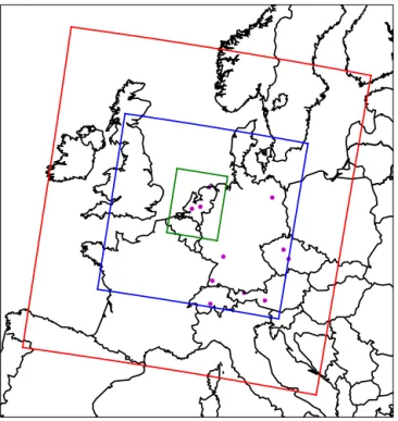
Figure 1.The location of modeled domains. The respective hori-zontal resolutions are according to the color of the domain bound-aries: red – 36 km×36 km; blue – 12 km×12 km; green – 4 km×
4 km. The scatter markers indicate the locations of various observa-tional sites used in this study.
Our biospheric fluxes (CO2r and CO2p) are generated
us-ing the SiBCASA model (Schaefer et al., 2008; van der Velde et al., 2014), which used meteorological fields from the European Centre for Medium-Range Weather Forecasts (ECMWF). It provides us with monthly averaged gross pho-tosynthetic production (GPP) and terrestrial ecosystem res-piration (TER) at 1◦×1◦resolution. Due to the coarse res-olution of the SiBCASA model, we find land-use categories in the higher resolution map of WRF that are not in the nat-ural land-use map of SiBCASA. To address this issue, we ran 9 simulations with SiBCASA prescribing a single veg-etation category, alternating through all the vegveg-etation cate-gories to produce biospheric fluxes for the different land-use categories within the resolution of WRF. For temporal inter-polation of the monthly fluxes, we scale the GPP and TER with the instantaneous WRF meteorological variables (tem-perature at 2 m and shortwave solar radiation) following the method described in Olsen and Randerson (2004).
Anthropogenic (fossil fuel) CO2 emissions (CO2ff) are
from the Institute for Energy Economics and the Rational Use of Energy (IER, Stuttgart, Pregger et al., 2007) at a hor-izontal resolution of 5 (geographical) minutes over Europe in the form of annual emissions at the location and temporal profiles to add variability during different months, weekdays and hours during the day. These are then aggregated to every WRF domain horizontal resolution and updated every hour
for the duration of our simulation. The emissions are intro-duced only at the lowest (surface) level of the model.
Anthropogenic (nuclear) 14CO2 emissions (14CO2n) are
obtained by applying the method described in Graven and Gruber (2011) for the year of 2008. We used information from the International Atomic Energy Agency Power Re-actor Information System (IAEA PRIS, available online at http://www.iaea.org/pris) for the energy production of the nu-clear reactors in our domain and reported14CO2discharges
for the spent fuel reprocessing sites (van der Stricht and Janssens, 2010). The data is available only on annual scale and once converted from energy production to emissions of 14CO2, these are scaled down to hourly emissions,
as-suming continuous and constant emission during the year. This is likely true when the nuclear reactors are operating, however, in reality regular maintenance and temporary shut-downs of individual reactors would result in periods of weeks and sometimes months of lower energy production and sub-sequently lower14CO2discharge. We will further comment
on these assumptions in our Discussion (Sect. 4).
2.3 Integrated114CO2air and plant samples
Integrated114CO2samples (1absorption), where the sampling
rate is usually constant (e.g. in various CO2absorption
se-tups), are represented with the concentration-weighed time-average114CO2signature for the period and height of
sam-pling, as seen in Eq. (7). When actual sampling is restricted to specific wind conditions or times-of-day, we include this in our model sampling scheme as well.
1absorption= X
t
1tobs CO t 2obs P
t
COt2obs (7)
Plant samples (1plant) integrate the atmospheric114CO2
signature with CO2assimilation rate which varies depending
on various meteorological and phenological factors. Photo-synthetic uptake and the allocation of the assimilated CO2
in the different plant parts strongly depend on the weather conditions and plant development. To simulate such samples we use WRF meteorological fields in the crop growth model SUCROS2 (van Laar et al., 1997) and use the modeled daily growth increment as a weighting function (averaging kernel) on the daytime atmospheric114CO2signatures (Bozhinova
et al., 2013). For each location we use the same sowing date and the model simulates the crop development until it reaches flowering, when we calculate 1plant. More explicitly these
integrated sample signatures are calculated as follows:
1plant= X
t
1tobsPXt t
Xt
, (8)
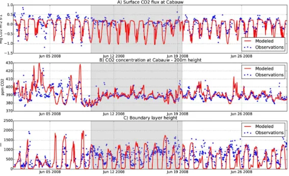
Figure 2.Comparison between modeled and observed CO2fluxes, concentrations and boundary layer height for the location of Cabauw for
one month in the simulated season. Performance is usually better on clear days as compared to cloudy ones, as indicated in the graph with the gray background.
3 Results
3.1 Model evaluation – how realistic are our CO2 and
114CO2simulations?
The meteorological conditions for 2008 that were simu-lated by WRF and used for the plant growth simulation in SUCROS2 were previously assessed in Bozhinova et al. (2013). Here we assess the model performance compared to observed CO2 fluxes, CO2 mole fractions, and
bound-ary layer heights. Figure 2 shows this comparison at the ob-servational tower of Cabauw, the Netherlands (data avail-able at http://www.cesar-observatory.nl). The simulated net CO2flux (NEE) compares well to observations with a
root-mean squared deviation (RMSD) of 0.26 mg CO2m−1s−1
and correlation coefficient (r) for the entire period of 0.70, which is even higher in clear days. Overestimates of NEE occur during cloudy conditions, which are notoriously diffi-cult to represent in many mesoscale models. The CO2mole
fractions compare well to observations (Vermeulen et al., 2011) and overall model performance is similar to other studies for the region (Tolk et al., 2009; Meesters et al., 2012). Similar to Steeneveld et al. (2008), Tolk et al. (2009), Ahmadov et al. (2009) the night-time stable boundary layer poses a challenge to the model. Note that the skill at mod-eling the boundary layer height can be of a particular im-portance for the correct simulation of the CO2 budget, as
it controls the diurnal evolution of the CO2mole fractions
(Vilà-Guerau de Arellano et al., 2004; Pino et al., 2012). Thus, we have included this comparison in the last panel of Fig. 2. More detailed statistics for this and other stations
and observations are listed in Table 1. We show the mean difference between the predicted and observed time series, with the according RMSD, and calculated correlation coef-ficient and coefcoef-ficient of determination (Willmott, 1982) for each location. While in Table 1 we show the statistics for the daily time-series, we also evaluated their hourly and daytime-only counterparts and the differences between each. Overall, our comparison shows that although the model overestimates the night-time CO2concentrations, it captures the observed
daytime CO2mole fractions features and their variability on
scales of hours to days satisfactorily over the full period sim-ulated for Cabauw.
We next analyze the results for the 114CO2 signature
corresponding to these CO2 mole fractions to evaluate our
skill at modeling the large scale 14CO2 over Europe.
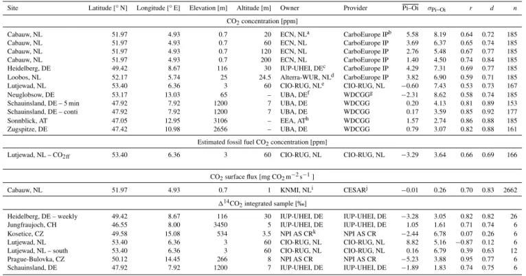
Table 1.The observational sites with data used in this study and statistics for the daily concentrations of CO2and CO2ffestimated from
CO observations, hourly flux CO2and monthly integrated114CO2observations as compared with modeled results. Here Pi–Oi represents the mean model-data difference andσPi–Oiis the spread of this difference. Both expressions carry the units described in the header of each
section.r anddare respectively the Pearson’s coefficient of correlation and the coefficient of determination.nis the number of members used in the statistical analysis.
Site Latitude [◦N] Longitude [◦E] Elevation [m] Altitude [m] Owner Provider Pi–Oi σ
Pi–Oi r d n
CO2concentration [ppm]
Cabauw, NL 51.97 4.93 0.7 20 ECN, NLa CarboEurope IPb 5.58 8.19 0.64 0.72 185
Cabauw, NL 51.97 4.93 0.7 60 ECN, NL CarboEurope IP 3.69 6.37 0.65 0.74 185
Cabauw, NL 51.97 4.93 0.7 120 ECN, NL CarboEurope IP 2.76 5.48 0.67 0.77 185
Cabauw, NL 51.97 4.93 0.7 200 ECN, NL CarboEurope IP 1.40 4.50 0.74 0.84 185
Heidelberg, DE 49.42 8.67 116 30 IUP-UHEI, DEc CarboEurope IP 4.29 7.31 0.69 0.77 185 Loobos, NL 52.17 5.74 25 24.5 Alterra-WUR, NLd CarboEurope IP 3.82 6.90 0.59 0.71 185 Lutjewad, NL 53.40 6.36 3 60 CIO-RUG, NLe CIO-RUG, NL −0.60 7.43 0.53 0.73 167
Neuglobsow, DE 53.17 13.03 65 – UBA, DEf WDCGGg −2.31 8.62 0.58 0.74 185
Schauinsland, DE – 5 min 47.92 7.92 1200 7 UBA, DE WDCGG 0.20 4.13 0.81 0.89 153 Schauinsland, DE – conti 47.92 7.92 1200 7 UBA, DE WDCGG 0.17 3.59 0.85 0.92 177
Sonnblick, AT 47.05 12.95 3106 – EEA, ATh WDCGG 1.57 2.74 0.86 0.88 185
Zugspitze, DE 47.42 10.98 2656 – UBA, DE WDCGG 0.79 3.07 0.82 0.88 161
Estimated fossil fuel CO2concentration [ppm]
Lutjewad, NL – CO2ff 53.40 6.36 3 60 CIO-RUG, NL CIO-RUG, NL −3.29 3.64 0.66 0.69 166
CO2surface flux [mg CO2m−2s−1]
Cabauw, NL 51.97 4.93 0.7 1 KNMI, NLi CESARj −0.01 0.26 0.70 0.83 2662
114CO2integrated sample [‰]
Heidelberg, DE – weekly 49.42 8.67 116 30 IUP-UHEI, DE IUP-UHEI, DE −3.28 3.05 0.82 0.82 26 Jungfraujoch, CH 46.55 8.00 3450 5 IUP-UHEI, DE IUP-UHEI, DE 1.05 1.61 0.71 0.74 6 Kosetice, CZ 49.58 15.08 534 3.5 NPI AS CRk NPI AS CR −2.44 6.78 0.07 0.26 6
Lutjewad, NL 53.40 6.36 3 60 CIO-RUG, NL CIO-RUG, NL 8.82 5.16 −0.87 0.12 6
Lutjewad, NL – south 53.40 6.36 3 60 CIO-RUG, NL CIO-RUG, NL 0.16 6.79 0.39 0.63 12 Prague-Bulovka, CZ 50.12 14.45 266 8 NPI AS CR NPI AS CR −5.23 3.88 0.95 0.77 6 Schauinsland, DE 47.92 7.92 1200 7 IUP-UHEI, DE IUP-UHEI, DE −1.89 1.83 0.74 0.75 6 aECN – Energy Research Center of the Netherlands, the Netherlands; contact person – Alex Vermeulen, [email protected]
bCarboEuropeIP – CarboEurope Integrated Project; http://www.carboeurope.org
cIUP-UHEI – Institute of Environmental Physics, University of Heidelberg, Germany; contact person – Ingeborg Levin, [email protected] dAlterra-WUR – Alterra, Wageningen University, the Netherlands; contact person – Eddy Moors, [email protected]
eCIO-RUG – Center for Isotope Research, University of Groningen, the Netherlands; contact person – Harro Meijer, [email protected] fUBA, DE – Federal Environmental Agency, Germany; contact person – Karin Uhse, [email protected]
gWDCGG – World Data Center for Greenhouse Gases; http://ds.data.jma.go.jp/gmd/wdcgg/
hEEA, AT – Environmental Agency Austria, Austria; contact person – Marina Fröhlich, [email protected] iKNMI – Royal Netherlands Meteorological Institute, the Netherlands; contact person – Fred Bosveld, [email protected] jCESAR – Cabauw Experimental Site for Atmospheric Research, the Netherlands; http://www.cesar-observatory.nl
kNPI AS CR – Nuclear Physics Institute, Academy of Sciences of the Czech Republic, Czech Republic; contact person – Ivo Svetlik, [email protected]
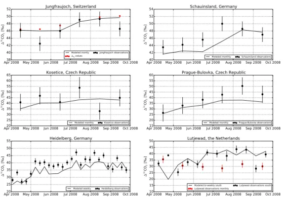
described in Turnbull et al. (2009b) we sampled a model layer in the free troposphere instead of at the modeled sur-face to better represent the observations. At all other sites we sample the pressure-weighted signature of the boundary layer, applying a minimum boundary layer height of 350 m during the night to avoid sampling too low surface signa-tures in a too stable nighttime boundary layer. The com-parison shows we capture reasonably well the seasonal cy-cle for most sites, however the model generally underesti-mates the114CO2. This is partly caused by the omitted
bio-spheric disequilibrium term, which accounts on average for up to 1.5 ‰ at these latitudes. Additional bias could be intro-duced through our choice of background site. In their study, Turnbull et al. (2009b) showed that the signature of free tro-pospheric air in the northern-hemispheric mid-latitudes can vary within 3 ‰ and additionally the signatures at mountain background sites (as Jungfraujoch) are slightly influenced by local fossil fuel emissions.
In the lowest left panel of Fig. 3 we show the comparison for Heidelberg, where observations are collected as weekly
night-time (between 19:00 and 07:00 local time) integrated samples. On higher temporal resolution our model estimates reproduce the temporal variations of the observations well. Still, the already discussed underestimation in 114CO2 is
also present at this site, which is located near a large ur-ban area with considerable fossil fuel emissions. During the period from May to August, this underestimation is on av-erage 5 ‰ in the model (∼1.8 ppm of fossil fuel CO2). In
the lowest right panel of Fig. 3 we show the comparison between the observed and modeled signatures at Lutjewad for the wind-specific measurements at this site in addition to the observed monthly samples that were continuously in-tegrated. The monthly114CO2observations for 2008 from
this location show atypical seasonality with a lack of the ex-pected summer maximum, and 10 to 20 ‰ lower114CO2
than the observations in Jungfraujoch and Schauinsland in that year. Although this suggests a large fossil fuel CO2
sig-nal for 2008, we could not find further evidence of this in the rest of the Lutjewad observational record (CO, CO2),
Apr 2008 May 2008 Jun 2008 Jul 2008 Aug 2008 Sep 2008 Oct 200838 40 42 44 46 48 50 52 ∆ 14CO 2 [ ] Jungfraujoch, Switzerland Modeled montly
∆bg values
Jungfraujoch observations
Apr 2008 May 2008 Jun 2008 Jul 2008 Aug 2008 Sep 2008 Oct 200840 42 44 46 48 50 52 54 ∆ 14CO 2 [ ] Schauinsland, Germany
Modeled monthly Schauinsland observations
Apr 2008 May 2008 Jun 2008 Jul 2008 Aug 2008 Sep 2008 Oct 200820 25 30 35 40 45 50 55 60 65 ∆ 14CO 2 [ ]
Kosetice, Czech Republic
Modeled monthly Kosetice observations
Apr 2008 May 2008 Jun 2008 Jul 2008 Aug 2008 Sep 2008 Oct 200815 20 25 30 35 40 45 50 55 60 ∆ 14CO 2 [ ]
Prague-Bulovka, Czech Republic
Modeled monthly Prague-Bulovka observations
Apr 2008 May 2008 Jun 2008 Jul 2008 Aug 2008 Sep 2008 Oct 200820 25 30 35 40 45 50 55 ∆ 14CO 2 [ ] Heidelberg, Germany
Modeled weekly Heidelberg observations
Apr 2008 May 2008 Jun 2008 Jul 2008 Aug 2008 Sep 2008 Oct 200810 15 20 25 30 35 40 45 50 ∆ 14CO 2 [ ]
Lutjewad, the Netherlands
Modeled bi-weekly south
Lutjewad observations monthly Lutjewad observations south
Figure 3.Comparison between observed and modeled atmospheric114CO2integrated samples for six observational sites. Red circles in the Jungfraujoch graph show the monthly fit used as the signature of the background CO2(1bg) in our calculations. Observations are monthly
continuously integrated samples at Jungfraujoch, Schauinsland, Kosetice, and Prague. At Heidelberg the weekly samples integrate only during the night-time. At Lutjewad the bi-weekly samples only integrate during periods of southerly winds, and the monthly integral over all sectors (discussed in the main text) is shown in red.
et al., 2010), which our model matches rather well. Since the measurements themselves seem valid, this feature in the continuous monthly Lutjewad 114CO2 data remains
unex-plained. We will however take a closer look at the temporal variability of the different114CO2components and the
gen-eral model performance at Lutjewad for the more accurately simulated southerly wind sector.
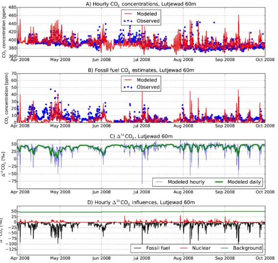
Figure 4 shows the 6-month hourly comparison of sim-ulated and observed CO2 and fossil derived CO2for
Lutje-wad. The latter is derived from14C-corrected high-resolution CO observations (van der Laan et al., 2010). Statistics for the comparison are also shown in Table 1. The fossil fuel sig-nal dominates over any variability in the background, clearly defining periods with enhanced transport of fossil fuel CO2
to the location (late April, start of May, start of July, start of August) as compared to less polluted air transported from the North Sea (mid-May, mid-June). The larger mismatch in particular periods (second half of April, start of May) can be attributed to the specific way the CO observations are cal-ibrated using the 3-year fit of the 14C-CO ratio at the site. While this would ensure that on an annual scale the actual
14C-CO relation is reached, on the bi-weekly scale of the 14C observations this sometimes results underestimation of
the14C-CO ratio compared to the observed values and con-sequently overestimation of the estimated fossil fuel CO2.
For more information, see van der Laan et al. (2010).
In the last panels we see this influence on the resulting 114CO2signature and especially its high temporal
variabil-ity that is not captured in the typically integrated monthly samples. Note that even though station Lutjewad is far away from nuclear emission sources, the signal from nuclear ac-tivity (shown in the last panel) can sometimes be of the same order of magnitude as the fossil fuel signal. This shows that it is important to evaluate the nuclear influence at every mea-surement site using a model like presented here, as it will contribute to the uncertainty in the recalculation of fossil fuel CO2.
3.2 Fossil fuel vs. nuclear emissions influence
on114CO2
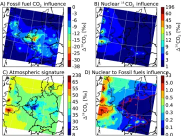
The lowest 114CO2 values in the domain are modeled in
the regions with high fossil fuel emission in Germany (the Ruhrgebiet), and the highest114CO2is near the large
emit-ting sites in western France and UK. This pattern can be clearly seen in Fig. 5a–c where results averaged over the lower 1200 m of the atmosphere over the full 6 months are shown. Note that the nuclear enrichment reaches much higher amplitude than the opposite effect by the fossil CO2,
but its influence on the atmospheric114CO2 is usually
Figure 4.6 months of hourly results for Lutjewad at 60 m height. Comparison between observed and modeled(a)CO2concentrations,
(b)CO2ffconcentrations(c)atmospheric114CO2and(d)the contribution of different compounds for the resulting114CO2. The transport
of air that is enriched in fossil fuel CO2is directly connected to the variations in the114CO2signal at the location, but these are not captured
by current observations due to their low temporal resolution.
part of our domain, where it captures the influence from the spent fuel reprocessing plant in La Hague (France) and several newer generation nuclear reactors in the UK. Even then, the influence of the nuclear enrichment averaged over 6 months is typically about 1 to 6 ‰ in areas that are not in direct vicinity of the sources. As a comparison, the fossil fuel influence in our domain on the same temporal and spa-tial scale is mostly between−3 and−15 ‰ outside the very polluted area of the Ruhrgebiet, Germany.
As the nuclear enrichment will (partially) mask the effect of fossil fuel CO2on the atmospheric114CO2, we show in
Fig. 5d the average 6-month ratio of the influences due to nu-clear and fossil fuel sources in our domain. Again, in most of the eastern and central parts of our domain the nuclear influ-ence is less than 10 % the fossil fuel influinflu-ence. This differs from the western part of our domain, where the ratio varies between 3 times smaller to about the same magnitude as the fossil fuel contribution and even to a more than 5 times larger influence in the area around the nuclear sources. The area
affected depends on the strength of the source, and in our case the influence of most water-cooled reactors rarely ex-ceeds the grid cell of the source, while for the gas-cooled re-actors the influence can be seen up to 50 km distance. These findings are consistent with Graven and Gruber (2011). The magnitude of the enrichment and size of the area influenced are both highly variable and strongly dependent on the atmo-spheric transport. As a result, in months with dominant east-erly winds the nuclear enrichment has a minimum effect in our domain, as most of the nuclear emissions are transported towards the Atlantic ocean and out of our area of interest. However, in months with dominant westerly winds, which is the prevailing wind direction, the nuclear14CO
2spreads
widely over the domain.
Figure 5.Spatial distribution for the 6-month averaged(a)fossil fuel CO2emissions influence,(b)nuclear14CO2emissions
influ-ence,(c)resulting114CO2signature in the atmosphere and(d)the
ratio between the nuclear and fossil fuel influences on the spheric signature, all averaged over the lower 1200 m of the atmo-sphere. While the largest influence over Europe is from fossil fuel CO2, the effect of the nuclear emissions of14CO2can be of
com-parable magnitude for large areas in France and UK.
70 % confidence interval of the emission factors (“low esti-mate” and “high estiesti-mate” runs). In Fig. 6 we show these re-sults as the absolute difference when compared to the mean run. While our largest source of nuclear emissions – lo-cated in La Hague, France, has directly reported emissions of14CO
2and is thus not subject to uncertainty in the
emis-sion factors, considerably higher or lower14CO
2signatures
could be associated with the nuclear estimates in the United Kingdom, southern Germany and central France.
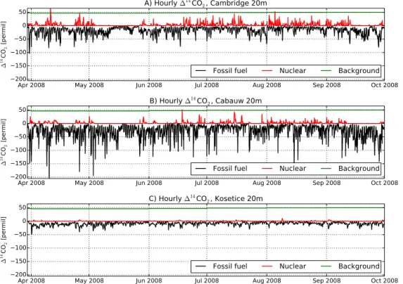
For sites located in northern and central France, southern Germany and the UK the nuclear enrichment means that cor-rections are needed that account for the nuclear influence in the observed 114CO2 before estimating the fossil fuel
influence. As an illustration, we show in Fig. 7 the influ-ence of the different anthropogenic emissions for three lo-cations with different characteristics in our domain: Cam-bridge (UK), Cabauw (the Netherlands) and Kosetice (Czech Republic). The locations were chosen to be in rural or agri-cultural areas, without large local CO2emissions. As seen in
Fig. 7, the western part of our domain (represented by Cam-bridge) has an equal influence from fossil fuel and nuclear emissions; the center (represented by Cabauw) experiences some events with relatively high nuclear emissions influence, but is influenced mostly by the very high fossil fuel emis-sions in this region (on average about 3 times higher than in Cambridge). In the east (represented by Kosetice) there is no significant signal of influence of nuclear emissions, but the influence of fossil fuel emissions is also considerably lower.
3.3 114CO2plant vs. atmospheric samples
In our previous work (Bozhinova et al., 2013) we described a method to model the114CO2in plant samples as the first
step in quantifying the differences between such samples and integrated atmospheric samples. Here we build on this work by calculating the plant signature resulting from uptake of spatially and temporally variable atmospheric114CO2. The
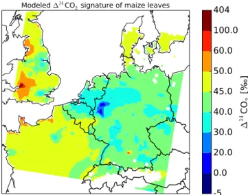
results for modeled samples from maize leaves at flowering, are shown in Fig. 8. Clearly, spatial gradients in114CO2in
plants are sizeable compared to the measurement precision of approximately 2 ‰. The regions with high influence from anthropogenic emissions from Fig. 5, namely the Ruhrgebiet in western Germany and the Benelux are also visible in the modeled plant signature, and so are some hot spots around larger european cities, like Frankfurt, Paris, London and oth-ers. It is important to point out that in addition to fossil fuel and nuclear gradients, plants develop at a different rate in different parts of the domain, and even the different parts of a plant (roots, stems, leaves, fruits) grow during different time periods.
The plant-sampled114CO2includes the effect of the
co-variance between the atmospheric 114CO2 variability and
the variability in the assimilation of CO2 in the plant
dur-ing growth, which is absent in traditional integrated samples where the absorption of CO2is based on constant flow rate
through an alkaline solution and thus only varies with the CO2 concentration present in the flow (Hsueh et al., 2007).
In Fig. 9 (left) we show this effect of the plant growth on the resulting plant114CO2 signature when comparing the
resulting plant signature with the daytime atmospheric aver-age we provide to our crop model. We should stress, that this is the magnitude of the error one should expect if the plant-sampled114CO2is assumed equal to the atmospheric mean 114CO2for the growing period of the plant. For many parts
of Europe in our simulated period this error is approaching the measurement precision of the114CO2 analysis (of
ap-proximately ±2 ‰). In the region located between the ar-eas with high fossil fuel and large nuclear emitters, however, the magnitude of the error can be several times larger. This is likely due to the absorption of some very high signature values in periods when the wind direction is directly from the nuclear source. Actual plant samples, taken during dif-ferent period than the one investigated here (namely 2010– 2012), will be used to further investigate these signatures in a follow-up publication.
Nuclear 14CO2 influence at
the surface in control run
0 1 2 3 4 5 10 25 50 184
∆
14CO
2
[
]
Absolute difference with high estimate results
0 1 2 3 4 5 10 50
∆
14CO
2
[
]
Absolute difference with low estimate results
0 1 2 3 4 5 10 50
∆
14CO
2
[
]
Figure 6.Spatial distribution for the uncertainty in the nuclear14CO2influence simulated for August and September, due to the uncertainty
in the emission factors associated with different reactor types. (Left) The nuclear influence modeled with the central estimate of the reactor emission factors; (middle) the absolute difference between the lower estimate and central estimate; (right) the absolute difference between the higher estimate and the central estimate. Low and high estimates refer to the 70 % confidence interval for the emission factors.
Apr 2008 May 2008 Jun 2008 Jul 2008 Aug 2008 Sep 2008 Oct 2008 200
150 100 50 0 50
∆
14CO
2
[p
ermi
l]
A) Hourly ∆14CO
2, Cambridge 20m
Fossil fuel Nuclear Background
Apr 2008 May 2008 Jun 2008 Jul 2008 Aug 2008 Sep 2008 Oct 2008 200
150 100 50 0 50
∆
14CO
2
[p
ermi
l]
B) Hourly ∆14CO
2, Cabauw 20m
Fossil fuel Nuclear Background
Apr 2008 May 2008 Jun 2008 Jul 2008 Aug 2008 Sep 2008 Oct 2008 200
150 100 50 0 50
∆
14CO
2
[p
ermi
l]
C) Hourly ∆14CO
2, Kosetice 20m
Fossil fuel Nuclear Background
Figure 7.Time series for the relative importance of nuclear vs. fossil fuel influence on the resulting atmospheric114CO2for three locations in our domain – near Cambridge (UK), Cabauw (the Netherlands) and Kosetice (Czech Republic).
to correctly account for nuclear influences such as through a modeling system could be important.
3.4 Direct estimation of the fossil fuel CO2emissions
While the entire emission map of Europe might be difficult to verify, most of the fossil fuel CO2 emissions are
pro-duced at only a number of locations. For instance, 10 % of all emissions in our domain come from only 30 grid cells and more than half of these are located in densely populated cities or urban conglomerations. This might provide an op-portunity for a better fossil fuel estimate of the highest emit-ting regions in Europe even when only selected locations
are visited in a plant sampling campaign. One could for in-stance assume that the114CO2signatures in plants in these
high-emission areas directly reflect the local anthropogenic sources, and a straightforward determination of their14CO2
signature would suffice to estimate emissions using a sim-ple box-model approach. We show in the following analysis that this simplification can lead to large errors though, and a more complete modeling framework like ours is needed for a proper interpretation of114CO2.
Modeled ∆14CO
2 signature of maize leaves
-5
0.0
20.0
30.0
40.0
45.0
50.0
60.0
100.0
404
∆
14
CO
2
[
]
Figure 8.Modeled absolute114CO2signature of maize leaves at flowering. Both the highly industrialized areas in Germany, where the atmospheric114CO2is lower than the background, and the
en-riched areas near the big nuclear sources in France and UK are vis-ible also in the plants. Even on this resolution we see in the plant signature the hot spots around Paris, London, Frankfurt, and many other big cities.
emissions over a 60 km×60 km area around 25 large Euro-pean cities, mix them through a 500 m deep boundary layer (typical 24 h average for our domain), and assume the air to have a residence time of 3.3 h (corresponding to a typical wind speed of 5 ms−1through a 60 km domain), we can make
a simple estimate of the resulting114CO2signature relative
to the background from Jungfraujoch. This box-model esti-mate is shown in Fig. 10 as the continuous straight line, in which the downward slope with increasing emissions is con-trolled mostly by the assumed residence time and the pre-scribed boundary layer height.
If we compare this linear relationship with the simulated 114CO2signatures over these cities simulated with the full
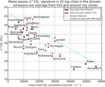
model developed in this paper (including its detailed hor-izontal advection, vertical mixing, and nuclear influence), one can see the large variability and substantial bias one would incur using the simple box-model approach. Up to 8 ‰ differences from this line would be found for Paris and Cologne, while the nuclear influence would lift Birming-ham plant samples back toward the Jungfraujoch background 114CO2despite its emissions being similar to Berlin. Even
if the full model-derived slope of approximately −4.85 ‰ per 10 000 mol km−2h−1could be reproduced with the
box-model, the coefficient of determination (R2) would be just over 0.7, meaning that close to 30 % of the spatial variance in emissions across Western Europe will not be captured in the simple approach. We therefore caution strongly against a simplified quantitative interpretation of114CO2signatures,
both in plants and in the atmosphere.
Figure 9.Difference between114CO2modeled in plants and the
daytime atmospheric average (left) and between modeled plants with and without taking the nuclear influence into account (right). While the left figure shows the error that should be expected if the plant growth is not taken into account and the plant signature is as-sumed to be equal to the atmospheric average, the right one shows the error that will be introduced if nuclear emissions of14CO2are not accounted for in the model simulation.
With a typical 114CO2 single measurement precision
of about ±2 ‰ and the full model-derived slope given above, we can tentatively estimate that even a perfect modeling framework will have a remaining uncertainty of 4000 mol km−2h−1for area-average emissions in these
top-25 emitters over Europe. This is quite substantial (20–50 %) for most of them, with the possible exception of the cities in the German Ruhr area (5–15 %). We therefore see an im-portant role for a monitoring program of114CO2signatures
in which emissions from all major sources are captured in multiple samples from multiple locations to minimize depen-dence on single observations and single atmospheric trans-port conditions. A modeling framework that can capture the specific characteristics of the regional atmospheric transport, fossil fuel emissions, and nuclear contributions like the one presented here would bring added value to the interpretation of such data.
4 Discussion
Our modeling results show that over a significant part of our domain, the nuclear influence on the atmospheric114CO2
signature will be more than 10 % (ratio=0.1 on Fig. 5d) of the estimated fossil fuel influence, introducing consider-able uncertainty to the method of using114CO2to calculate
the fossil fuel CO2addition to the regional atmosphere. The
strongest gradients of114CO2in Western Europe are found
in the relatively polluted region in western Germany and the Netherlands due to the high population density and large in-dustry sector there, and hence high CO2emissions. As was
shown for California by Riley et al. (2008), more detailed
14CO
2observations in this region can possibly prove useful
0 10000 20000 30000 40000 50000 60000 Fossil Fuel CO2 emissions [mol km−2 h−1]
10 15 20 25 30 35 40 45 50
∆
14CO
2
[
]
Paris
Dortmund Bremen
Rotterdam Dresden Sheffield
Munich
Berlin Leeds Hamburg
Birmingham
Brussels Nuremberg
Hannover
Dusseldorf Stuttgart
Frankfurt
The Hague Prague
Leipzig
Cologne London
Amsterdam Copenhagen
Essen
Maize leaves
∆14CO
2
signature in 25 top cities in the domain,
emissions are average from 5x5 grid around city center
Only fossil fuel influence Fossil fuel and nuclear 14CO2
Nuclear influence Simple estimate with 500m BLH
Figure 10.Comparison between the results of the simple box model (see main text) and the modeled maize leaves114CO2signature at
city center and fossil fuel CO2 emissions averaged for 5×5 grid
around the city center on 12 km horizontal resolution.
ensures that uncertainties arising from nuclear emissions will be at their minimum.
This result relies partly on the underlying emission maps for the anthropogenic (fossil fuel) CO2and (nuclear)14CO2
emissions. We should consider various factors that are un-certain or unknown at this point for these emissions (Peylin et al., 2011; Graven and Gruber, 2011) – such as temporal characters, vertical resolution and even small irregularities in the spatial allocation of the emission sources. All our an-thropogenic emissions are currently introduced in the lowest (surface) layer of our model, but according to the emission database used (IER, Stuttgart), most of the industrial emis-sion stacks are located on average at 100 to 300 m height. Using this information in our model will likely result in the emitted CO2being transported away faster, and result in less
local enrichment. This is also true for our nuclear emissions sources, but information on their vertical emission heights is more difficult to find.
For the fossil fuel CO2emissions we apply temporal
pro-files that disaggregate monthly, weekly and diurnal signals from the provided annual emissions. For the nuclear emis-sions such profiles are unknown and information on their temporal heterogeneity is not publicly available. In this study we consider these emissions as continuous and constant throughout the year. This is a relatively safe assumption for the emissions from nuclear power plants as their 14CO2 is
a by-product of the normal operation of the reactor. Tempo-rary shutdowns for scheduled maintenance that covers peri-ods of weeks and sometimes months would invalidate this as-sumed emission pattern. Continuous constant emissions are not likely for reprocessing sites, where the emissions will depend on the type and amount of fuel being reprocessed.
Additionally, there is uncertainty if these emissions are re-leased continuously or in a few large venting events, where the venting procedures are moreover likely to be reactor-type dependent. Currently, we lack the information to account for such complications.
When using flask samples for 14CO2 measurement
nu-clear enrichment can relatively easily be recognized. How-ever, in integrated air and plant samples this signal will be av-eraged over the total sampling period. Depending on weather variability, local fossil fuel CO2addition and the proximity
to the nuclear sources, the enrichment in 114CO2 can
of-ten be within the measurement precision (of approximately ±2 ‰) as we have shown. Thus, integrated samples likely have too low time resolution and sensitivity to attribute nu-clear emissions, and areas where this influence is high would profit from flask sampling of114CO2 in addition to
inte-grated plant sampling. Because plant samples can be used only as complementary observations during particular sea-sons and depending on the species sampled a dual monitor-ing approach with flasks and integrated samples seems best. Based on our results, a better characterization of the tempo-ral structure of the nuclear emissions is a prerequisite for any
14CO
2-based monitoring effort in Europe.
Our study is subject to known uncertainties in atmo-spheric transport of mesoscale models. An inaccurate sim-ulation of wind speed and direction (Lin and Gerbig, 2005; Gerbig et al., 2008; Ahmadov et al., 2009) or boundary layer height development (Vilà-Guerau de Arellano et al., 2004; Steeneveld et al., 2008; Pino et al., 2012) will affect the transport of emission plumes and resulting mole fractions. Resolving more meso-scale circulations, and improved rep-resentation of topography can be particularly advantageous, as they can cause large gradients in CO2(de Wekker et al.,
2005; van der Molen and Dolman, 2007). While WRF-Chem is used for a variety of atmospheric transport studies (among others: Tie et al., 2009; de Foy et al., 2011; Lee et al., 2011; Stuefer et al., 2013), more general air quality studies have shown that an ensemble of models can forecast air pollu-tion situapollu-tions more accurately than a single model (Gal-marini et al., 2004, 2013). While in our research we fo-cused on the transport of CO2and14CO2, other chemically
active tracers (e.g. CO, NOx) that are regularly measured
and connected with anthropogenic emissions could be used too. Including222Rn as an additional tracer can help low-ering the uncertainty associated with the vertical mixing in the model and provide correction factors to be applied to the other passive tracers, as shown in van der Laan et al. (2010), Vogel et al. (2013).
Considering future uses of114CO2observations as
addi-tional constraint on the carbon cycle, we should note that at-mospheric inversions currently typically use only afternoon observational data. In that case, plant-sampled114CO2
ob-servations may provide a better representation of the af-ternoon atmospheric114CO2signals than conventional
However, the use of plant samples is typically limited to the summertime, which is a period with lower anthropogenic CO2 emissions, more vertical mixing and larger biospheric
fluxes. This will correspond to larger uncertainty in the recal-culation of the fossil fuel CO2emissions compared to
win-tertime.
We explored the possibility that a relatively simple box-model can be used to calculate the emissions directly from 114CO2observations, and showed its inability to capture the
variability in114CO2signals across 25 European cities.
Us-ing such a simple box model has high inherent uncertainty for the reconstructed emissions, a portion of which is a direct consequence of the114CO2measurement precision.
Our results suggest that a combination of the available sampling methods should be used when planning a 14CO2
observational network for fossil fuel emissions estimates. In-tegrated air and plant samples alone can provide a longer pe-riod observations at a lower cost, but are less useful for eval-uation of large nuclear influences in shorter periods. Flask samples are much better suited for this, however their con-tinuous analysis is too costly. A possible compromise could be to obtain flask samples for a limited period alongside integrated samples for new sampling locations. This would already provide information about the possible nuclear en-richment and the wind directions from which it usually oc-curs. Additionally, while integrated air samples are the cur-rent standard for quasi-continuous observations of 14CO2,
plant samples can be obtained at a much higher spatial reso-lution without additional infrastructure investment. Their use is however constrained to the sunlit part of the day and gen-erally the summer season, and the exact time and locations where the chosen crop grows.
5 Conclusions
In this work, we demonstrated the ability of our modeling framework to simulate the atmospheric transport of CO2
and consequently the atmospheric114CO2 signature in
in-tegrated air and plant samples in Western Europe. Based on our results we reach the following conclusions.
1. Simulated spatial gradients of114CO2are of
measur-able size and the 6-month average CO2ffconcentrations
in the lower 1 km of the atmosphere across Western Eu-rope are between 1 to 18 ppm.
2. Enrichment by14CO2from nuclear sources can partly
mask the Suess effect close to nuclear emissions, par-ticularly in large parts of UK and northwestern France. This is consistent with previous studies (Graven and Gruber, 2011) and we show that in these regions the strength of the nuclear influence can exceed the influ-ence from fossil fuel emissions.
3. The simulated plant 114CO2 signatures show spatial
gradients consistent with the simulated atmospheric
gradients. Plant growth variability induces differences between the simulated plant and the daytime atmo-spheric mean for the period of growth, of a magni-tude that is mostly within the measurement precision of ±2 ‰, but can be up to±7 ‰ in some areas.
4. Integrated114CO2samples from areas outside the
im-mediate enrichment area of nuclear emission sources are not sensitive to occasional advection of enriched air due to their long absorption period. However, to prop-erly account for the nuclear enrichment term on smaller time scales, improvements in temporal profiles of nu-clear emissions are needed.
5. New114CO2 sampling strategies should take
advan-tage of different sampling methods, as their combined use will provide a more comprehensive picture of the atmospheric114CO2temporal and spatial distribution.
Acknowledgements. This work is part of project (818.01.019), which is financed by the Netherlands Organisation for Scien-tific Research (NWO). Further partial support was available by NWO VIDI grant (864.08.012). We acknowledge IER (Stuttgart, Germany) for providing the anthropogenic CO2emissions maps,
IAEA PRIS for the nuclear reactor information and NCEP and ECMWF for the meteorological data. We thank I. Levin (University of Heidelberg), I. Svetlik (Academy of Sciences, Czech Repub-lic)A. Vermeulen (ECN), S. Palstra and R. Neubert (CIO), E. Moors (Alterra), M. Fröhlich (EAA, Austria), K. Uhse (UBA, Germany) and F. C. Bosveld (KNMI) for providing the observational data used in this study. We further want to thank H. Graven (Imperial College London, UK), N. Gruber (Swiss Federal Institute of Tech-nology, Switzerland), and I. van der Laan-Luijkx and M. Combe (Wageningen University, the Netherlands) for the scientific support and useful comments provided for this manuscript.
Edited by: M. Heimann
References
Ahmadov, R., Gerbig, C., Kretschmer, R., Körner, S., Röden-beck, C., Bousquet, P., and Ramonet, M.: Comparing high res-olution WRF-VPRM simulations and two global CO2 trans-port models with coastal tower measurements of CO2,
Biogeo-sciences, 6, 807–817, doi:10.5194/bg-6-807-2009, 2009. Anderson, E., Libby, W., Weinhouse, S., Reid, A., Kirshenbaum, A.,
and Grosse, A.: Natural Radiocarbon from Cosmic Radiation, Phys. Rev., 72, 931–936, doi:10.1103/PhysRev.72.931, 1947. Bozhinova, D., Combe, M., Palstra, S., Meijer, H., Krol, M., and
Peters, W.: The importance of crop growth modeling to interpret the114CO2signature of annual plants, Global Biogeochem. Cy.,
27, 792–803, doi:10.1002/gbc.20065, 2013.
de Foy, B., Burton, S. P., Ferrare, R. A., Hostetler, C. A., Hair, J. W., Wiedinmyer, C., and Molina, L. T.: Aerosol plume trans-port and transformation in high spectral resolution lidar mea-surements and WRF-Flexpart simulations during the MILA-GRO Field Campaign, Atmos. Chem. Phys., 11, 3543–3563, doi:10.5194/acp-11-3543-2011, 2011.
de Wekker, S. F. J., Steyn, D. G., Fast, J. D., Rotach, M. W., and Zhong, S.: The performance of RAMS in representing the con-vective boundary layer structure in a very steep valley, Environ. Fluid Mech., 5, 35–62, doi:10.1007/s10652-005-8396-y, 2005. Djuricin, S., Pataki, D. E., and Xu, X.: A comparison of tracer
meth-ods for quantifying CO2sources in an urban region, J. Geophys.
Res.-Atmos., 115, D11303, doi:10.1029/2009JD012236, 2010. Dudhia, J.: Numerical study of convection observed during the
Win-ter Monsoon Experiment using a mesoscale two-dimensional model, J. Atmos. Sci., 46, 3077–3107, 1989.
Ek, M., Mitchell, K., Lin, Y., Rogers, E., Grunmann, P., Koren, V., Gayno, G., and Tarpley, J.: Implementation of NOAH land sur-face model advances in the National Centers for Environmental Prediction operational mesoscale Eta model, J. Geophys. Res.-Atmos., 108, 8851, doi:10.1029/2002JD003296, 2003.
Francey, R., Trudinger, C., van der Schoot, M., Law, R., Krum-mel, P., Langenfelds, R., Steele, L. P., Allison, C., Stavert, A., Andres, R., and Rodenbeck, C.: Atmospheric verification of an-thropogenic CO2 emission trends, Nature Climatic Change, 3,
520–524, doi:10.1038/nclimate1817, 2013.
Friedlingstein, P., Houghton, R., Marland, G., Hackler, J., Bo-den, T., Conway, T., Canadell, J., Raupach, M., Ciais, P., and Quéré, C. L.: Update on CO2emissions, Nat. Geosci., 3, 811– 812, 2010.
Galmarini, S., Bianconi, R., Addis, R., Andronopoulos, S., As-trup, P., Bartzis, J., Bellasio, R., Buckley, R., Champion, H., Chino, M., D’Amours, R., Davakis, E., Eleveld, H., Glaab, H., Manning, A., Mikkelsen, T., Pechinger, U., Polreich, E., Pro-danova, M., Slaper, H., Syrakov, D., Terada, H., and Auw-era, L. V. D.: Ensemble dispersion forecasting – Part II: Applica-tion and evaluaApplica-tion, Atmos. Environ., 38, 4619–4632, 2004. Galmarini, S., Kioutsioukis, I., and Solazzo, E.:E pluribus unum:
ensemble air quality predictions, Atmos. Chem. Phys., 13, 7153– 7182, doi:10.5194/acp-13-7153-2013, 2013.
Gerbig, C., Körner, S., and Lin, J. C.: Vertical mixing in atmo-spheric tracer transport models: error characterization and prop-agation, Atmos. Chem. Phys., 8, 591–602, doi:10.5194/acp-8-591-2008, 2008.
Graven, H. D. and Gruber, N.: Continental-scale enrichment of at-mospheric14CO2from the nuclear power industry: potential
im-pact on the estimation of fossil fuel-derived CO2, Atmos. Chem. Phys., 11, 12339–12349, doi:10.5194/acp-11-12339-2011, 2011. Graven, H. D., Guilderson, T. P., and Keeling, R. F.: Observations of radiocarbon in CO2at La Jolla, California, USA 1992–2007:
Analysis of the long-term trend, J. Geophys. Res.-Atmos., 117, D02302, doi:10.1029/2011JD016533, 2012a.
Graven, H. D., Guilderson, T. P., and Keeling, R. F.: Observa-tions of radiocarbon in CO2 at seven global sampling sites in the Scripps flask network: Analysis of spatial gradients and seasonal cycles, J. Geophys. Res.-Atmos., 117, D02303, doi:10.1029/2011JD016535, 2012b.
Gurney, K., Mendoza, D., Zhou, Y., Fischer, M., Miller, C., Geethakumar, S., and Can, S. D.: High resolution fossil fuel
com-bustion CO2emission fluxes for the United States, Environ. Sci.
Technol., 43, 5535–5541, 2009.
Hsueh, D. Y., Krakauer, N. Y., Randerson, J. T., Xu, X., Trum-bore, S. E., and Southon, J. R.: Regional patterns of radiocarbon and fossil fuel-derived CO2in surface air across North America,
Geophys. Res. Lett., 34, L02816, doi:10.1029/2006GL027032, 2007.
Koffi, E. N., Rayner, P. J., Scholze, M., Chevallier, F., and Kamin-ski, T.: Quantifying the constraint of biospheric process pa-rameters by CO2concentration and flux measurement networks
through a carbon cycle data assimilation system, Atmos. Chem. Phys., 13, 10555–10572, doi:10.5194/acp-13-10555-2013, 2013. Kuc, T., Rozanski, K., Zimnoch, M., Necki, J., and Korus, A.: An-thropogenic emissions of CO2and CH4in an urban environment,
Appl. Energ., 75, 193–203, 2003.
Lee, S.-H., Kim, S.-W., Trainer, M., Frost, G. J., McKeen, S. A., Cooper, O. R., Flocke, F., Holloway, J. S., Neuman, J. A., Ryer-son, T., Senff, C. J., SwanRyer-son, A. L., and ThompRyer-son, A. M.: Mod-eling ozone plumes observed downwind of New York City over the North Atlantic Ocean during the ICARTT field campaign, Atmos. Chem. Phys., 11, 7375–7397, doi:10.5194/acp-11-7375-2011, 2011.
Levin, I. and Hesshaimer, V.: Radiocarbon – a unique tracer of global carbon cycle dynamics, Radiocarbon, 42, 69–80, 2000. Levin, I. and Karstens, U.: Inferring high-resolution fossil fuel CO2
records at continental sites from combined14CO2and CO
ob-servations, Tellus B, 59, 245–250, 2007.
Levin, I. and Kromer, B.: Twenty years of atmospheric14CO2
ob-servations at Schauinsland station, Germany, Radiocarbon, 39, 205–218, 1997.
Levin, I. and Rödenbeck, C.: Can the envisaged reductions of fossil fuel CO2emissions be detected by atmospheric observations?,
Naturwissenschaften, 95, 203–208, 2008.
Levin, I., Munnich, K., and Weiss, W.: The effect of anthropogenic CO2 and 14C sources on the distribution of14C in the
atmo-sphere, Radiocarbon, 22, 379–391, 1980.
Levin, I., Schuchard, J., Kromer, B., and Munnich, K. O.: The con-tinental European Suess effect, Radiocarbon, 31, 431–440, 1989. Levin, I., Kromer, B., Schmidt, M., and Sartorius, H.: A novel approach for independent budgeting of fossil fuel CO2 over Europe by14CO2 observations, Geophys. Res. Lett, 30, 2194,
doi:10.1029/2003GL018477, 2003.
Levin, I., Hammer, S., Kromer, B., and Meinhardt, F.: Radiocarbon observations in atmospheric CO2: determining fossil fuel CO2
over Europe using Jungfraujoch observations as background, Sci. Total. Environ., 391, 211–216, 2008.
Levin, I., Naegler, T., Kromer, B., Diehl, M., Francey, R. J., Gomez-Pelaez, A. J., Steele, L. P., Wagenbach, D., Weller, R., and Wor-thy, D. E.: Observations and modelling of the global distribution and long-term trend of atmospheric14CO2, Tellus B, 62, 26–46,
doi:10.1111/j.1600-0889.2009.00446.x, 2010.
Levin, I., Kromer, B., and Hammer, S.: Atmospheric114CO2trend
in Western European background air from 2000 to 2012, Tellus B, 65, 20092, doi:10.3402/tellusb.v65i0.20092, 2013.