Designed by the Bio-Inspired
Physarum
Algorithm
Shin Watanabe, Atsuko Takamatsu*
Department of Electrical Engineering and Bioscience, Waseda University, Shinjuku-ku, Tokyo, Japan
Abstract
In this paper, we propose designing transportation network topology and traffic distribution under fluctuating conditions using a bio-inspired algorithm. The algorithm is inspired by the adaptive behavior observed in an amoeba-like organism, plasmodial slime mold, more formally known as plasmodium of Physarum plycephalum. This organism forms a transportation network to distribute its protoplasm, the fluidic contents of its cell, throughout its large cell body. In this process, the diameter of the transportation tubes adapts to the flux of the protoplasm. ThePhysarumalgorithm, which mimics this adaptive behavior, has been widely applied to complex problems, such as maze solving and designing the topology of railroad grids, under static conditions. However, in most situations, environmental conditions fluctuate; for example, in power grids, the consumption of electric power shows daily, weekly, and annual periodicity depending on the lifestyles or the business needs of the individual consumers. This paper studies the design of network topology and traffic distribution with oscillatory input and output traffic flows. The network topology proposed by thePhysarumalgorithm is controlled by a parameter of the adaptation process of the tubes. We observe various rich topologies such as complete mesh, partial mesh, Y-shaped, and V-shaped networks depending on this adaptation parameter and evaluate them on the basis of three performance functions: loss, cost, and vulnerability. Our results indicate that consideration of the oscillatory conditions and the phase-lags in the multiple outputs of the network is important: The building and/or maintenance cost of the network can be reduced by introducing the oscillating condition, and when the phase-lag among the outputs is large, the transportation loss can also be reduced. We use stability analysis to reveal how the system exhibits various topologies depending on the parameter.
Citation:Watanabe S, Takamatsu A (2014) Transportation Network with Fluctuating Input/Output Designed by the Bio-InspiredPhysarumAlgorithm. PLoS ONE 9(2): e89231. doi:10.1371/journal.pone.0089231
Editor:Dante R. Chialvo, National Research & Technology Council, Argentina
ReceivedOctober 23, 2013;AcceptedJanuary 16, 2014;PublishedFebruary 26, 2014
Copyright:ß2014 Watanabe, Takamatsu. This is an open-access article distributed under the terms of the Creative Commons Attribution License, which permits unrestricted use, distribution, and reproduction in any medium, provided the original author and source are credited.
Funding:This work is partly supported by a grant of Strategic Research Foundation Grant-aided Project for Private Universities from MEXT, No. S1001027 and Grant-in-Aid for JSPS Fellows, No. 24.4255. The funders had no role in study design, data collection and analysis, decision to publish, or preparation of the manuscript.
Competing Interests:The authors have declared that no competing interests exist. * E-mail: [email protected]
Introduction
Transportation networks such as power grids are, in general, designed under certain static supply-demand conditions. However, in most situations, whether the network is that of nature or a man-made system, the inputs/outputs into/from the networks fluctuate rather than remain constantly static. One such example is an ant foraging trail network, in which ants cannot constantly prey upon their foods because the activities of the prey animals fluctuate daily or seasonally. The feature also holds for man-made networks. For instance, the number of passengers commuting by rail is maximized in the mornings and evenings and the peak times shift among stations in suburbs and city areas on weekdays. Addition-ally, the transportation patterns on weekends are quite different from those on weekdays. The second man-made example is power grids. The pattern of electricity consumption is distributed according to the lifestyles or business style of consumers, which was recently confirmed using clustering analysis on a town in Japan [1]. More specifically, the consumption pattern fluctuates daily, weekly, and seasonally, and the peak time depends on the consumers.
Optimization of networks under fluctuating conditions is difficult to be conducted in a straightforward manner by conventional
methods within linear- and nonlinear-programming frameworks. In this paper, we propose designing traffic distribution in networks under fluctuating conditions using an algorithm inspired by the
organismPhysarum.
ThePhysarumalgorithm, which mimics the shortest path-finding behavior of the plasmodial slime mold organism [2], formally
calledPhysarum polycephalum, was developed by Tero et al. [3]. The
plasmodium of Physarum is a giant amoeba-like multinucleated
unicellular organism. It contains thousands of nuclei, so the cell
size can get very large, ranging from 10mm to 1 m. To distribute
protoplasm, including nutrients, oxygen, and organelles, through-out this large cell body, the organism has developed a peculiar transportation network consisting of tubular structures. The diameter of the tubes adapts to the flux of the protoplasm: The tubes on the paths connecting multiple food sites become thick in accordance with the growth of the protoplasmic flow, while the other paths become thin and finally disappear when there is little or no flow. Consequently, the organism is able to generate the
shortest paths connecting multiple food sites [2,4]. ThePhysarum
in wireless sensor networks [8]. Although, in the above examples, it was applied under static conditions, the algorithm can also be applied under fluctuating conditions owing to its adaptive behavior.
This paper studies the design of network topology and traffic distribution under oscillating conditions, which is the simplest type of fluctuating environment. The network consists of nodes and links, which, in power grids for example, correspond to consumers, power plants, electric poles, and power lines. A multiplicity of consumers uses electricity with daily periodicity (oscillating condition). The peak consumption times vary according to the consumers, and are defined by phase lags.
In the Methods section, we outline how thePhysarumalgorithm
is modified to deal with problems involving oscillating conditions and define performance functions. We then present the network
designs under oscillating conditions proposed using the Physarum
algorithm and evaluate them using our performance functions, in the Results section. In the Discussion section, a stability analysis for a simple network is considered in our discussion of the numeric result. Finally, we discuss the effect of the oscillating condition and the phase lags.
Methods
PhysarumAlgorithm
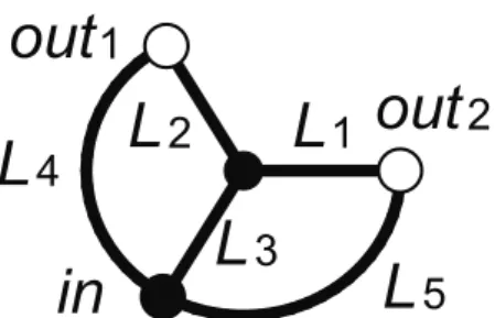
In this section, we modify the originalPhysarumalgorithm [3] to
deal with the example network depicted in Fig. 1. The shaded and unshaded large circles, respectively, represent nodes for input
(denoted as in) and output (denoted as out1,2) of transported
materials, such as protoplasm inPhysarum, current in power grids,
and people in railroad grids. The linklij connecting the nodesi
andjhas the following properties: lengthLij, conductivityDij, and
traffic volume flux Qij. Their meanings in each application are
summarized in Table 1.
The flux at each node conserves
P i
Qij~
0, j=in,out1,2,
{Iin, j~in,
Iout1,2, j~out1,2,
ð1Þ
whereIin andIout1,2 are the fluxes at inandout1,2, respectively.
The total flux to/from the system should be balanced:
Iin~Iout1zIout2: ð2Þ
The fluxQijis given by
Qij~Dij
Lij(pi{pj) , ð3Þ
wherepiandpjrepresent, respectively, the pressure at nodesiand
j. Substituting Eq. (3) for Eq. (1),piis obtained under the givenLij
Figure 1. Network topology used by thePhysarumalgorithm for numerical calculation. doi:10.1371/journal.pone.0089231.g001
Table 1.Correspondence of variables.
Variables General Physarum Power Grid
Lij length of link length of tube length of electric wire Dij conductivity tube thickness
(!r4 ij)
electric conductivity (!r2
ij) Qij flux of traffic
volume
flux of protoplasm current
andDij.Qijis then calculated using Eq. (3) again. In the numerical calculations,Lij~1:0is set at all links.
As mentioned in the introductory section, the conductanceDij
adapts to flux. Therefore, the conductance is assumed to evolve according to the following differential equation:
dDij
dt ~f(jQijj){Dij, ð4Þ
meaning that the tube grows depending on the flux (the first term on the right hand side of the equation) while it degenerates (the second term). It is natural in biological systems for the growth rate
to be saturated by an upper limit. Thus, function f(:) can be
defined as a sigmoid function:
f(jQijj)~ jQijj m
1zjQijjm : ð5Þ
This function is widely found in biological cooperative processes
[9]. The parametermis the key parameter governing the dynamics
of this system. Whenmw1, the tube grows only slightly when the
flow is extremely weak, although the growth speed is accelerated when it once starts to grow, then it is finally saturated at one.
When m~1, the function is categorized into the Michaelis–
Menten type, which represents the simplest enzymatic reaction. Whenmv1,f(:)represents fast initial growth and slow saturation, suggesting no meaning related to biological processes.
Application to Networks with Oscillating Conditions
The outputs atout1,2are assumed to oscillate as follows:
Iout1~1zsinvt, Iout2~1zsin (vtz ) , ð6Þ
where v is angular frequency and represents a phase lag
between the outputs. In Eq. (6),v~2p|102is assumed so that
the period of oscillationT~2p=v~10{2is small enough to the
time constant of the degeneration process of Dij, which is
estimated as one. We confirmed that the outline of the results in
this paper is valid over the frequency range
2p|10{1ƒvƒ2p|107, namely, over the period range
10{7ƒTƒ101(see}1 in File S1 for details).
Converged Value of Dij
We repeat the computation of Eq. (4) with Eqs. (1)–(3), and Eq.
(6) until Dij converges within a certain accuracy. In fact, Dij
continues to oscillate slightly even after a long evolution period
(Figs. A and B in}1 in File S1). Therefore, the completion of the
convergence is judged according to the following criterion.
First, a variation amount ofDijat timetis defined as follows:
(t)~1
m X
ij
Dij(tznT){Dij(t)
2
, ð7Þ
where n(~100) is the number of cycles in the input/output
oscillation, andmis the total number of links. The convergence of
Dijis judged to be complete when (t)vc:10{26(the value ofec
is set by the reasoning below). Consequently, the averaged value
D
Dij at timetznT is calculated using the following definition:
D Dij(t)~1
T ðtzT
t
Dij(s)ds: ð8Þ
After the convergence is ascertained,DDij (t)is denoted asDDij~ . The link is removed (DDij~ set to zero) when DDij~ becomes less than a
certain threshold Dmin:10{13. The value is sufficiently smaller
than the order of the maximum value ofDijD~ (
~
110{1). Finally, thenetwork topologies and traffic distributions (magnitude of
conductances) recommended by the Physarum algorithm are
obtained (Figs. 2 and 3). Note that the threshold value for
judgment ofDij-convergence cis sufficiently smaller thanDmin.
Performance Functions
We now introduce three performance functions to evaluate the
performance of the networks recommended by the Physarum
algorithm: power or transportation loss, building and/or mainte-nance cost, and vulnerability in network topology.
(current)2|(electric resistance)in a wire.
Conseq-lij is defined asQ2
ij multiplied byLij=Dij~ }2
P~1
T ðT
0
X
ij Q2ij(t)
Lij
~
D Dij
( )
dt, ð9Þ
where the loss is averaged over a period of input/output oscillation becauseQij oscillates.
CostBis that for building and/or maintaining a network, which
is expected to be proportional to the total volume of the network.
Because the cross section of each link is proportional toDijin the
case of power grids, as described in Table 1, B is defined as
follows:
B~X
ij
LijDDij~ : ð10Þ
Note thatB~PijLij
ffiffiffiffiffiffi
~
D Dij q
should be adopted when
consider-ing the original Physarum network because the relation between
conductivity and a tube of radiusrij is described asDij!r4
ij (see
also Table 1) [3,6].
VulnerabilityVis defined as the probability that the connection
out1orout2frominis divided when one of the links in the network
is randomly deleted. The deletion frequency is assumed to be
proportional to the length of the link whenLij is not
homoge-neous, where the probability is normalized by the total length of
the network, Ltot. Consequently, the vulnerability is defined as
follows:
V~X
ij Gij Lij
Ltot , ð11Þ
where disconnectivityGijfor a linklijis set to one if transportation flows out fromincan reach neitherout1norout2; otherwise, it is
set to zero.
ϵ
Loss P is defined using an analogy to electric energy loss, which is
calculated with
Results
We considered two cases, constant and oscillating flux at input and output nodes, and evaluated the network topologies and traffic
distributions recommended by the Physarumalgorithm using the
three performance functions.
Constant Condition
Before capturing the effect of oscillatory input/output on the network design, we tested the effect with constant input/output. We set the fluxes to constant values,Iin~2,Iout1,out2~1, in Eq. (1).
The numerical calculation started from a homogeneous initial
condition ofDij~1:0or a non-homogeneous condition according
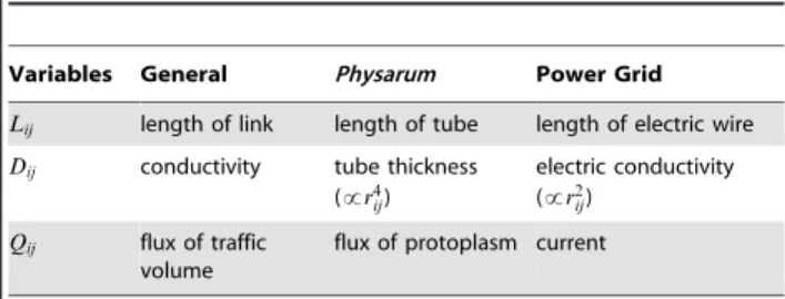
to normal distribution with mean 1.0 and standard deviation 0.1. We observed eight types of network topologies in the parameter range0vmƒ5:0as shown in Fig. 2.
The network topology changes from dense to sparse depending
on m. When m is smaller (m 1:4), the network forms a mesh
accompanied by circular structures (Figs. 2Aand 2B). When m
becomes larger (m 1:4), the network forms a tree structure
(Figs. 2Cand 2D). The mesh networks are categorized into two
types, complete mesh (type 1; Fig. 2A) and partial mesh (types 2–5;
Fig. 2B). The tree networks are categorized into two types,
V-shaped (types 6 and 7; Fig. 2C) and Y-shaped (type 8; Fig. 2D)
networks. The Y-shaped networks appear whenm 1:8. The paths
from the input are partially shared in the Y-shaped network, while they are directly connected to the two outputs in the V-shaped network.
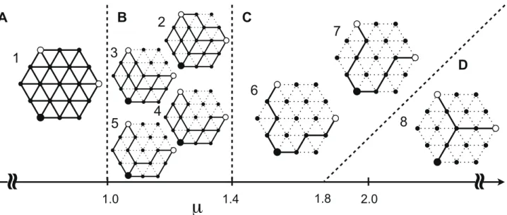
Oscillating Condition
We set the input/output flux oscillating using the definition in Eq. (6). The numerical calculation started from a homogeneous
initial condition of Dij~1:0 or non-homogeneous conditions
according to normal distribution with mean 1.0 and standard deviation 0.1. We observed 20 types of network topologies in the
parameter range0vmƒ5:0, as shown in Figs. 3, S1 and S2. In
this case, the dependence of network topology onmis similar to
that of the constant condition: when 0vmv1, complete mesh
(type 1) appeared. Asmincreased over 1, the topology changes to
partial mesh (types 2–5 and 9–19). Finally, when mw1:5,
V-shaped (types 6 and 7) or Y-V-shaped (type 8) networks were observed. It should be noted that the variation of the topologies becomes broader than in the case of the constant condition when
1 m 1:8: a variety of partial meshes, i.e., networks of types 9–19
besides types 2–5, were observed.
The network topology depends not only onmbut also on phase
lag and on the initial conditions ofDij. The characteristics are
particularly evident in mw1. Figure 4 shows the network types
observed according tom, , and the initial conditions ofDij. For
m 1:7, primarily partial meshes were observed (see Fig. S2 for
details). Dependence of the topology on can be seen more clearly
whenm 1:7: the V-shaped network is more frequently observed
Figure 2. Dependence of network topology under constant input and output.Initial values of Dij were either set as homogeneous (Dij~1:0for all links) or were distributed according to a normal distribution with mean 1.0 and standard deviation 0.1. Solid and dashed lines of the
network diagrams denote surviving and removed links, respectively.AComplete mesh (type 1),0vmv1.BPartial mesh (types 2–5),1ƒm 1:4.C V-shaped network (types 6 and 7),m 1:4.DY-shaped network (type 8),m 1:8. When the initial conditions ofDijare exactly homogeneous, the V-shaped network appears in the range of1:4 m 2:2and the Y-shaped network appears in the range ofm 2:3. Type numbers correspond to those of Figs. 3 and S1.
doi:10.1371/journal.pone.0089231.g002
Figure 3. Network types calculated with oscillating inputs and outputs.A type number is assigned to each topology. The full list of network topologies is represented in Fig. S1. The data are those for the homogeneous initial conditions ofDij. The plots of mesh, partial mesh, V-shaped and Y-shaped networks, are colored in black, red, blue, and green, respectively. The dependence of type of partial mesh on is shown in Fig. S2.
Figure 4. Relation between network types and the parametersmand under oscillating conditions. AHomogeneous initial condition of
Dij~1:0 {DExamples of non-homogeneous initial condition ofDij: Initial values ofDijwere distributed according to a normal distribution with
mean 1.0 and standard deviation 0.1. Black, gray, and white squares denote partial mesh, V-shaped and Y-shaped networks, respectively. The specific type-number of partial mesh depends on both parametersmand (Fig. S2), and also on the initial condition ofDij, which is not shown here in detail.
doi:10.1371/journal.pone.0089231.g004 B
Figure 5. Performance depending on parametersmand . ALossP.BCostB.C VulnerabilityV. Circles, triangles and squares denote performances when ~0,p=2,p, respectively. The crosses inCdenote the performances of the constant condition. The data are those for the homogeneous initial conditions ofDij. The case starting from non-homogeneous initial conditions is demonstrated in}3 in File S1.
when the two outputs are in phase ( *0) and the observation ratio of the Y-shaped network increases accordingly as the lag
approaches anti-phase ( *p). Note that the dependence of the
topology on is also subject to the initial distribution of Dij in
detail (compare the diagramsAof homogeneous condition andB–
Dof three different non-homogeneous conditions in Fig. 4).
Evaluation of the Networks
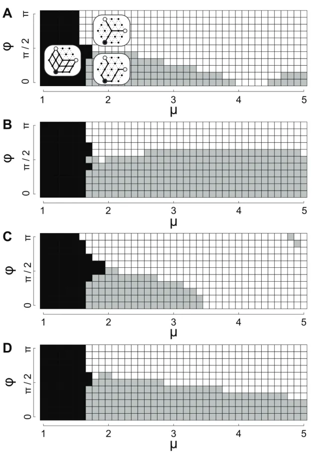
Figure 5 shows the performances P, B, and V estimated for
each combination of parametersmand , where each network is
calculated from the homogeneous initial conditions ofDij. Smaller
values mean better performances in these analyses. Loss P
increases until aroundm~1:7, then slightly decreases, irrespective
of , as shown in Fig. 5A. Notably,Pfor ~p is clearly always
smaller than those for ~0andp=2. The discontinuity in the plots
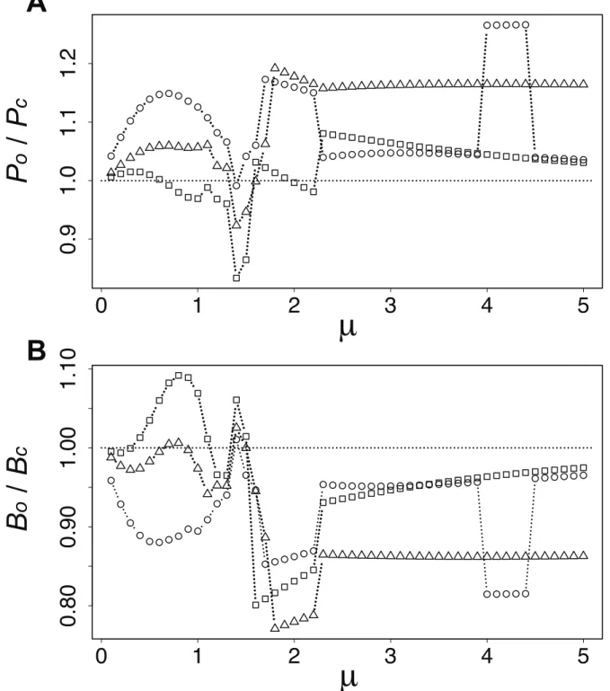
Figure 6. Comparison of the performances for the networks designed under constant and oscillatory conditions. ARatio in loss,
Po=Pc.BRatio in cost, Bo=Bc. Circles, triangles, and squares respectively denote ~0,p=2,p. The data are those for the homogeneous initial conditions ofDij.
for ~0when4 m 4:4is caused by the discontinuous change
of network topology. CostBdecreases rapidly until aroundm~1,
then it becomes almost constant, as shown in Fig. 5B.
Vulnera-bilityV equals0whenm 1:5, as shown in Fig. 5Cbecause the
network includes circular structures (Figs. 2A and B). Asmexceeds
around 1.5, V jumps to 1.0 because the network includes no
circular structure. In conclusion, the network is well balanced at
1 m 1:5. The results for the non-homogeneous initial conditions
ofDijare valid for virtually the same feature as in the case for the
homogeneous conditions (see}3 in File S1 for details).
Benefit Derived from the Introduction of Oscillatory Condition
To investigate the benefit derived from the introduction of the oscillatory condition, we calculated the ratio of the performances
between the constant and oscillatory input/output, as shown in
Fig. 6. Note that the performancePcandBcwere estimated with
oscillatory input/output against the networks obtained under
constant condition by thePhysarumalgorithm. The performances
Po and Bo were estimated with oscillatory input/output against
the networks obtained under the oscillatory condition, which are the same as those of Fig. 5.
A ratio with value smaller than 1.0 suggests that the performance of the network considering the oscillatory condition is better. LossPfor the oscillatory condition is better than that for
the constant condition only when1:4 m 1:5. In contrast, costB
almost always shows better performance in the oscillatory condition. The cost can be reduced to about 80% in the best
performance. The effect of vulnerability is captured in Fig. 5C:
Vulnerability is improved by considering the oscillatory condition
when1:3 m 1:8.
Discussion
Stability Analysis of Network Topology
To understand the parameter dependence of the network topology, we conducted stability analyses of network topologies and estimation of their basin size against a network with small compositions of nodes and links (Fig. 7).
In this subsection, the notation of linklij is redefined aslk. In accordance with this definition, the equations for conductances D~(D1, ,D5)are rewritten instead of using Eq.(4) as follows:
dDk
dt ~f(jQkj){Dk, k~1, ,5: ð12Þ Figure 7. The simple network used for stability analysis.The link
lengths were set as L1~L2~L3~1:0 andL4~L5~2:0so that any path length fromintoout1,2is 2.
doi:10.1371/journal.pone.0089231.g007
Figure 8. Twelve equilibria for the network in Fig. 7 represented in network-topology form. AComplete mesh,B–Fpartial mesh,G Y-shaped network,H–JV-shaped network,KandLthe others.
The equation (6) is redefined as Iout1~0:5(1zsinvt),
Iout2~0:5f1zsin (vtz )g, where the magnitude of the input/ output flux is set as half of those in Eq. (6) because the network size is now reduced.
In Eq. (12),Dkhas two time scales: slow and fast. The fast time
scale is caused byv, which gives fluctuations with small amplitude
toDk. Accumulation of the small asymmetric fluctuations finally
derives a slow drift inDk. The final network topology must be
determined mainly by the slow dynamics. Therefore,Dk can be
averaged over a period of the fast dynamics when we focus only on
slow dynamics, which is denoted as DDk hereafter. The slow
dynamics ofDDk can be written as follows:
dDDk
dt ~ffk{DDk:gk
where ffk:1 T
ðT
0
ffjQk(t)jgdt:
ð13Þ
The steady state of Eq. (13),dDDk
dt ~0, is considered then the
solutions of the equationgk~0, namely equilibria, are denoted as
D~ DD
1, ,DD5
. The magnitudes of individual elements ofD
determine the topology of the network. Note thatQk, and alsoffk,
are a function of DDk owing to Eq.(3). Therefore, we solved
equationgk~0using Newton’s method, whereffi is obtained by
numerical integration of f(:) according to the above definition
using Eqs. (1)–(3), (5). The integration offfjQk(t)gover the period
of output oscillation in Eq. (13) depends on because of the
nonlinearity of the function (see}4 in File S1 for details).
We obtained 12 equilibria of D, as summarized in Fig. 8,
where the topologies are drawn based on the magnitude of the elements’ values, DD
1, ,DD5. The topologies can be roughly
classified into complete mesh (Fig. 8A), partial mesh (Figs. 8B–F),
Y-shaped (Fig. 8G), V-shaped (Figs. 8H–J) networks, and others
(Figs. 8K and L) similar to those of Fig. 2 and S1. The V-shaped
network is, furthermore, divided into subcategories: symmetric
(Fig. 8H, denoted by the V-shaped network in Fig. 9), and
asymmetric (Figs. 8I–J, denoted by the V9-shaped network in
Fig. 9).
We conducted linear stability analysis for each equilibriumD.
The Jacobian matrixJofg~(g1, ,g5)is defined using Eq. (13)
as follows:
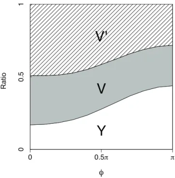
Figure 9. Observation ratio for small network.The network in Fig. 7 was used. Y, V, and V9respectively denote the network topologies represented in Figs. 8G, 8H, and 8I–J. The parameterm~2:0was set. In each calculation against , all combinations amongDi~0:1,0:2, ,1:0 for all linksi~1,2, ,5(specifically, a total of105combinations) were tested as initial conditions. The networks such as the ones shown in Fig. 8KandLwere also observed but the observation ratios were extremely small, e.g., 0 when 0ƒ ƒ0:7p, 0.002 when ~0:8p, 0.018 when
~0:9p, and 0.03 when ~p. doi:10.1371/journal.pone.0089231.g009
Figure 10. Maximum eigenvalues depending on when ~0.Circles, triangles, and squares, respectively, denotelmaxat the equilibria of
complete mesh (Fig. 8A), partial mesh (Fig. 8E), and Y-shaped (Fig. 8G). Crosses representltc for V-shaped (Fig. 8H) networks.
doi:10.1371/journal.pone.0089231.g010
Jkl ~ Lgk
LDDl , k,l~1, ,5
~ Lffk
LDDl { LDDk
LDDl
~ Lffk
LDDl {1 (k~l),
Lffk
LDDl (k=l):
ð14Þ
Because it is difficult to calculate Eq. (14) directly, we estimated
the Jacobian matrix at D (denoted as J hereafter) using the
following approximate form:
Lffk
LDDl
j
D~D^
ffk(DzDDl){ffk(D)
jDDlj , ð15Þ
whereDDlis a vector with anl-th element valueddand the others
zero, e.g., DD2~(0,d,0,0,0). For the numerical calculation,
d~10{5 was used. We then calculated the eigenvalues for J,
l1, , l5. When max½Re(l1), ,Re(l5):lmaxv0, the
equi-libriumDis determined as stable.
The above method is not appropriate to examine whether the
V-shaped network (Fig. 8H) is globally stable because changing the
V-shaped network (Fig. 8G) to other network types, such as complete
or partial mesh (Fig. 8A, D, E, orF), requires at least two additional links. In Eq. (14), only a single additional link can be considered. Therefore, instead of calculating eigenvalues, we estimate a time
constant ltc converging to D from a vicinity. We tested four
combinations of deviations from the V-shaped equilibrium, (d,d,d,d,d), (d,d,d,d,{d), (d,d,d,{d,d), (d,d,d,{d,{d). Finally,
we defined the maximum time constant asltc.
Figure 10 summarizes the dependence of the maximum
eigenvalues lmax (or ltc for the V-shaped network) on the
parameter m. The single stable equilibrium, complete mesh, is
found in the region ofmƒ1:0. The complete mesh remains stable
overmw1:0followed by participation of the Y-shaped, V-shaped,
and partial mesh networks. The complete and partial meshes
become unstable whenm exceeds 1.3. The stability change from
complete mesh, via partial mesh, to Y-shaped or V-shaped network resembles that of the larger network (Fig. 3). However, no significant difference can be found in the features of the stability
among different phase-lags ~0, p=2 and p (Fig. S3) while
appearance of Y-shaped or V-shaped network apparently depends
on in the larger network, as seen in Fig. 4. The dependence
would be caused by the difference in the basin sizes between the Y-shaped and V-Y-shaped networks. Figure 9 shows the observation
ratio of the Y-shaped and the V-shaped networks. Both types are always observed but the ratio of the Y-shaped network increases in
accordance with . The change in basin size depending on could
explain the observation that the Y-shaped network is more frequently observed in anti-phase lag in the larger network, as seen in Fig. 4.
Summary and Conclusion
In this paper, we proposed using the Physarum algorithm to
design transportation network topologies and traffic distribution under oscillating conditions. The results of numerical experiments indicate that this approach is valid and has the following benefits:
1) Only one parameter m can control the morphology of the
network. The client using the network can choose a particular parameter according to which they consider to be the most important among loss, cost, and vulnerability.
2) By introducing oscillating condition, building and/or main-tenance cost is reduced to a maximum of 80% that of cases in which conditions are static.
3) Phase lag among outputs results in a wide variety of network
morphology when mw1 (sigmoidal growth in the
conduc-tance).
Table 2 summarizes the first item. Partial mesh can be recommended when the client requests a system with loss, cost, and vulnerability well-balanced. The third index, vulnerability, should be noted when considering power grids. The meshed network has a low vulnerability index but it includes loop connections, which are prone to cascading failure problems. When some nodes or links in a meshed network are damaged, the current that would normally go through those links must be distributed to the surrounding links. However, if the current goes beyond the capacity of the surrounding links, the damage
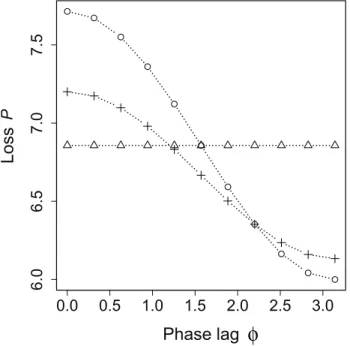
Figure 11. Relation between lossP and of small network. Circles, triangles, and crosses respectively denote Y-shaped network (Fig. 8G), V-shaped network (Fig. 8H), and complete mesh (Fig. 8A). The total volume ( = cost) for each network is normalized by that for the complete mesh so that the three networks are made with the same cost.
doi:10.1371/journal.pone.0089231.g011
Table 2.Evaluation of the network type for each item.
m
Network\
Evaluation Loss Cost Vulnerability Cascading
,1.0 Complete mesh A+
C A+
C
1.0–1.4 Partial mesh B A A+ C
.1.4 V-shaped or Y-shaped
B or C A+ C A+
Az: best, A: good, B: acceptable, C: bad.
propagates rapidly to the outer surrounding links. This results in large-scale blackouts [10,11]. Considering these phenomena, V-shaped and Y-V-shaped networks are recommended rather than partial mesh. For railroads and highways, in which cascades need not be considered, partial mesh can be recommended. The cascading problem was not treated as a performance function in this paper because, for the sake of simplicity, the capacity of the current for each link was not considered. This will be dealt with in future work.
For the second item, if a client considers the reduction of power loss more important than building and maintenance cost, a network that is designed under static conditions is recommended. The recommendation can be reversed by considering the third item, phase lag. Then, the problem of loss can be overcome.
For the third item, the Y-shaped network is observable more frequently than the V-shaped network as the phase lag gets larger
when mw1:4. This topological selection delivers a maximum of
20% loss reduction to the system. Notably, the loss decreases when the lag approaches anti-phase away from in-phase, as shown in Fig. 11. This result theoretically supports a justification of the ‘‘peak shift’’ action developed in Japan for reducing electric power after the Fukushima nuclear disaster in 2011. The peak shift action shifts usage of electricity from on-peak to off-peak periods. This allows the electric power consumption in power grid systems to flatten during the day and to be reduced in peak periods. By introducing this action, the number of standby power plants can be reduced: Such the plants, e.g., thermal ones, are on standby to regulate power generation flexibly and to avert power shortages in peak periods. Our results suggest that peak shift action contributes to a reduction in not only the number of standby power plants but also in power loss in the grid.
Natural systems may gain advantages by self-organizing their network. Argentine ants are known to make supercolonies, which consist of multiple colonies with a single family. They form V-shaped or Y-V-shaped trails connecting the multiple colonies [12]. Army ants build dendritic trails–large-scaled Y-shaped branching structures [13]. Tao et al. showed, by a computer simulation, that virtual ants building Y-shaped trails can gain more food than those building V-shaped trails when the foods appear in anti-phase at two sites [14]. By considering the number of ants as cost, the result can be interpreted as the ants selectively building Y-shaped
networks under constraints of constant cost and fluctuating environment. As a result of the selection, the ants can convey food with minimum loss. Of course, it is known that slime mold,
the model organism inspires the Physarum algorithm itself,
constructs Y-shaped, V-shaped and dendritic networks depending on environmental conditions [15–17]. The slime mold and the ants selected the optimum way without any systematic plan long before humans analyze such as these.
Supporting Information
Figure S1 Full list of network topologies with oscillating condition.The topology number corresponds to that of Figs. 2 and 3.
(EPS)
Figure S2 Relation between the types of partial mesh
and . 1ƒm 1:9. The type number corresponds to that of Fig.
S1. (EPS)
Figure S3 Maximum eigenvalues depending onm when
~0,p=2,p. A ~0.B ~p=2.C ~p. Circles, triangles, and
squares, respectively, denote lmax at the equilibria of complete
mesh (Fig. 8A), partial mesh (Fig. 8E), and Y-shaped (Fig. 8G).
Crosses representltcfor V-shaped (Fig. 8H) networks.
(EPS)
File S1 Footnotes. (PDF)
Acknowledgments
We thank Y. Hayashi, H. Shen, H. Hino, N. Murata, and S. Wakao of Waseda University for useful discussions about power grids and electricity consumption patterns. We also thank R. Kobayashi and K. Ito of Hiroshima University for stimulating discussions about the Physarum
transportation network and ant foraging trails.
Author Contributions
Conceived and designed the experiments: AT SW. Performed the experiments: SW. Analyzed the data: SW. Wrote the paper: SW AT.
References
1. Hino H, Shen H, Murata N, Wakao S, Hayashi Y (2013) A versatile clustering method for electricity consumption pattern analysis in households. IEEE Trans Smart Grid 4: 1048–1057.
2. Nakagaki T, Yamada H, Toth A (2000) Maze solving by an amoeboid organism. Nature 407: 470.
3. Tero A, Kobayashi R, Nakagaki T (2007) A mathematical model for adaptive transport network in path finding by true slime mold. J theor Biol 244: 553–564. 4. Nakagaki T, Yamada H, Toth A (2001) Path finding by tube morphogenesis in
an amoeboid organism. Biophys Chem 92: 47–52.
5. Tero A, Takagi S, Saigusa T, Ito K, Bepper DP, et al. (2010) Rules for biologically inspired adaptive network design. Science 327: 439–442. 6. Watanabe S, Tero A, Takamatsu A, Nakagaki T (2011) Traffic optimization in
railroad networks using an algorithm mimicking an amoeba-like organism, Physarumplasmodium. Biosystems 105: 225–232.
7. Adamatzky A (2010)PhysarumMachines: Computers from slime mold. World Scientific.
8. Li K, Thomas K, Torres C, Rossi L, Shen CC (2010) Slime mold inspired path formation protocol for wireless sensor networks. In Dorigo M et al., editors ANTS 2010, Heidelberg: Springer 299–311.
9. Keener JP, Sneyd J (1998) Mathematical physiology, Interdisciplinary Applied Mathematics, Vol. 8. Springer.
10. Sachtjen ML, Carreras BA, Lynch VE (2000) Disturbances in a power transmission system. Phys Rev E 61: 4877–4882.
11. Dobson I Carreras BA, Lynch VE, Newman DE (2007) Complex systems analysis of series of blackouts: Cascading failure, critical points, and self-organization. Chaos 17: 026103-1-026103-13.
12. Latty T, Ramsch K, Ito K, Nakagaki T, Sumpter DJT, et al. (2011) Structure and formation of ant transportation networks. J R Soc Interface 8: 1298–1306. 13. Burton JL, Franks NR (1985) The foraging ecology of the army antEction rapax
an ergonomic enigrama? Ecol Entomol 10: 131–141.
14. Tao T, Nakagawa H, Yamasaki M, Nishimori H (2004) Flexible foraging of ants under unsteadily varying environment (cross-disciplinary physics and related areas of science and technology). J Phys Soc of Jpn 73: 2333–2341. 15. Nakagaki T, Kobayashi R, Nishiura Y, Ueda T (2004) Obtaining multiple
separate food sources: behavioural intelligence in the Physarumplasmodium. Proc R Soc B: Biological Sciences 271: 2305.
16. Takamatsu A, Takaba E, Takizawa G (2009) Environment-dependent morphology in plasmodium of true slime moldPhysarum polycephalumand a network growth mode. J Theor Biol 256: 29–44.