431
Abstract
The geological modeling of stratiform deposits can become very complex, often making use of geological envelopes of small thickness and requiring the use of sub-blocks (based on Cartesian coordinates) to produce a coherent block model. However, geological events after the formation of the deposit (folds, faults, etc.) can change the direction of spatial continuity of certain attributes, with the mixing of samples belong-ing to different formation eras (in the case of stratiform deposits) in the same elevation. This study presents a solution for deposits with stratigraphic grades combined with samples of different origins. The solution is a two-dimensional estimate obtained by accumulating the thicknesses of P2O5 in a phosphate deposit (as compared to tradi-tional statistical analysis in three dimensions).
Keywords: accumulation, ordinary kriging, phosphate.
Resumo
A modelagem geológica de depósitos estratiformes pode-se tornar muito com-plexa, muitas vezes fazendo uso de envelopes geológicos de pequena espessura e exigindo o uso de sub-blocos (com base em coordenadas cartesianas) para produzir um modelo de blocos coerente. No entanto, eventos geológicos após a formação do depósito (dobras, falhas, etc.) podem mudar a direção da continuidade espacial de certos atributos, com mistura de amostras pertencentes a épocas de formação geoló-gicas diferentes (no caso de depósitos estratiformes) na mesma elevação. Esse estudo apresenta uma solução para depósitos com teores estratigráicos combinados com amostras de diferentes origens. A solução é uma estimativa bidimensional obtida pela acumulação da espessura de P2O5 em um depósito de fosfato (em comparação com a análise estatística tradicional em três dimensões).
Palavras-chave: acumulação, krigagem ordinária, fosfato.
Diego Machado Marques
Mining Engineer, MsC, PhD,
Mining Engineering Department, UFRGS, Porto Alegre, Rio Grande do Sul, Brasil [email protected]
Ricardo Hundelshaussen Rubio
Industrial Engineer, Msc, PhD Candidate, Mining Engineering Department, UFRGS, Porto Alegre, Rio Grande do Sul, Brasil [email protected]
João Felipe Coimbra Leite Costa
Mining Engineer, Msc, PhD.
Mining Engineering Department, UFRGS, Porto Alegre, Rio Grande do Sul, Brasil [email protected]
Evangelina Maria Apparicio da Silva
Mining Engineer, Msc, Vale S.A, Belo Horizonte, Minas Gerais, Brasil [email protected]
The effect of accumulation in
2D estimates in phosphatic ore
O efeito da acumulação em 2D
em estimativas de minério fosfático
Mining
Mineração
1. Introduction
The estimate of an attribute (grade, thickness, etc.) using geostatis-tical data requires certain assumptions, and among them is the assumption that the attribute presents autocorrelation in time and/or space. These estimates are based on temporal/spatial continuity for the attribute, which in turn is based on the sample values of the attributed model. In many cases, the database is geo-positioned using a Cartesian coordinate system. However, the
con-tinuity of the phenomenon may not be compatible with this type of coordinate. At the time of formation of mineral de-posits, the minerals are crystallized or deposited in positions consistent with an active geological process, and this process determines the continuity of at-tributes related to the constitution of the rocks (e.g. mineral grades). Geological events subsequent to the formation of the deposit, such as folding, can change the direction of continuity of certain
at-tributes (Koppe et al., 2006). There are some ways around this issue, such as coordinate transformations (McArthur, 1987; Deutsch, 2002) and accumulation in two dimensions (2D) (Krige, 1981).
432 REM: R. Esc. Minas, Ouro Preto, 67(4), 431-437, oct. dec. | 2014
it adds complexity to the estimation process. Besides requiring additional steps to obtain the inal grades, it can generate inconsistencies if not executed properly, with, for example, extreme values exceeding the minimum and maximum grades of the original data.
This article aims to present the steps in the estimation of a phosphatic deposit (P2O5) through the accumula-tion process in 2D, showing all the necessary steps for its implementation. In addition, the reasons for choosing to perform the estimation in 2D rather than the conventional three dimensions
(3D) are shown. The deposit studied had several layers of phosphatic ore interspersed with layers of waste rock.
The positions of the Highwall and the Footwall were determined using data from drillholes. The results of the modeling showed almost horizontal layers, with a slight folding, and large variations in thickness
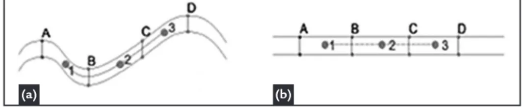
The determination of the spatial continuity of the deposit could be under-mined by mixing samples of the same level (elevation), Z, belonging to a dif-ferent geological formation era (distinct stratigraphic levels), correlating samples
that may be on the Highwall in a drill-hole at one given Z coordinate and on the Footwall in another drillhole at the same Z coordinate, as shown in Figure 2(a) (holes A, B, C and D). In view of this, the unfolding (transformation of Cartesian coordinates to stratigraphic coordinates) of the deposit could be a way of improving the results of the analysis of spatial continuity, given that in deposits of sedimentary origin, the values from sediments of the same geological age (stratigraphically on the same horizon) tend to have high spatial correlation (Figure 1 (b)).
Figure 1. Theoretical example of how folds in the geological phenomenon (a) may affect the analysis of spatial continuity, and (b) how unfolding of the layer can reduce the problem. It can be noted in (a) that, independent of the orientation of the ellipsoid search of samples, those of the same geological
era (1, 2 and 3) will be the same, if prop-erly analyzed. After the transformation (b), samples of the same geological era (1, 2 and 3) have the same orientation and coordinates in the search plan.
Finally, in certain cases, the Eu-clidean distance is an inadequate mea-sure (as in the Figure 2) and should be
replaced by, for example, a "curved" distance measurement in layers with folds (Dagbert et al. 1984).
To determine whether the study should be performed in 3D with sup-port, or in 2D, accumulating grades by the thickness, the series of tests pre-sented below were performed.
2. Methodology
The sample data from a drill-ing campaign were obtained from d r i l l c ore s of d i f f e re nt le n g t h s (different bases).
These data from distinct bases can be used for accurate geological modeling, but to estimate grades (from a statistical point of view) using them may create bias in the results.
The database provided for
geo-statistical modeling had a total of 1643 samples in the layer of interest. Because of the characteristics of the mineral deposit, it was impossible to regularize the bases of the samples, i.e. setting all the samples to a constant length for geostatistical analysis. In addition, the database was composed of data from four drilling campaigns, each with speciic goals and its own protocol for
sample preparation, taking no account of a standard sample size, varying be-tween 0.1 and 2.12 m.
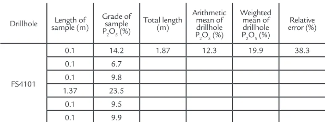
The bias created by the use of that data unmodiied is shown in Table 1, where data for a drillhole obtained by the fourth drilling campaign is shown. Note that the layers adjoining the con-tact region show a small sample thick-ness (some with high grade).
Figure 2
Cross section of
interest layer (north–south) 1000 2000 3000 4000 5000 6000 7000 8000
-20
-30
-40
-50
-60
Ele
vation (m)
Isatis
NE (m)
(a) (b)
433
Sample regularization usually in-volves combining existing sample values; i.e. it is a procedure that involves numeri-cal numeri-calculation of the weighted means of the grades in larger volumes than the original samples. Typically, such a com-position is linear in nature, involving calculation of a weighted mean of adjacent samples uniformly over a greater length than a single sample length (Sinclair and
Blackwell, 2002). Some of the common reasons for sample regularization are: to provide an equal basis (support) for geo-statistical analysis, and reduce the number of extreme values and the variability that these values may cause.
There are several different methods for the regularization that can be used, depending on the nature of the mineraliza-tion and type of mining process. Common
regularization methods are: regularization by the height of the bench, regularization by constant length, and regularization by ore zone.
The only method applicable (without breaking the samples into smaller inter-vals) is the regularization method by ore zone. The result of this adjustment may be seen in Figure 3, where each sample represents a drillhole.
Figure 3 Histogram of the length of the sample of interest after the regularization by ore zone.
After sampling regularization, it can be seen that there is a great variability in
thickness. Thus, a sample set does not ex-ist on the same basis, preventing a study in
3D without bias, as seen in the theoretical example shown in Figure 4 and Table 2.
Figure 4 Theoretical example of regularization by ore zone.
Drillhole sample (m)Length of Grade of sample P2O5 (%)
Total length (m)
Arithmetic mean of drillhole P2O5 (%)
Weighted mean of drillhole P2O5 (%)
Relative error (%)
FS4101
0.1 14.2 1.87 12.3 19.9 38.3
0.1 6.7
0.1 9.8 1.37 23.5
0.1 9.5
0.1 9.9
434 REM: R. Esc. Minas, Ouro Preto, 67(4), 431-437, oct. dec. | 2014
All possibilities were analyzed for correction of basis, to try to determine a method without bias, and the only pos-sible solution found by this study was the accumulation of the database in 2D. The following steps were performed:
• accumulation of all data by the
length of the sample;
• analysis of spatial continuity
of the accumulated variables and the length of the sample (thickness);
• deinition of the search strategy
for estimation;
• estimation of cumulative and
variable thickness;
• validation of estimates; • de-accumulation;
• validation of the results of the
de-accumulation.
3. Accumulation
The regionalized variables (VRs) must be such that all linear combina-tions of their values keep the same mean. If f(x) represents the grade of a sample, the sum of samples multiplied by their weight (in this example, the length of the sample), Σiλi*f(xi), is the arithmetic mean (1/n)*Σif(xi), which must have the same mean grade (Journel and Huijbregts, 1978).
The process of regularization en-sures that the sample regionalized
vari-ables have the same length and therefore the same basis, which is necessary for the implementation and use of geostatistical analysis. But in some cases, this is not enough (e.g. chemical variables associ-ated with particle size fractions) or not applicable (e.g. small, thick layers of ore). In the case of a thin layer of iron ore, one usual method of estimation is the use of an auxiliary variable obtained by multiplying the grade by the thickness (i.e. accumula-tion). The estimated grades are obtained
indirectly by the relationship between the estimated cumulative variable and the esti-mated thickness. This practice stems from variations in the basis (thickness) and the problem of the non-additive nature of the content of the resulting variable (Marcotte and Boucher, 2001).
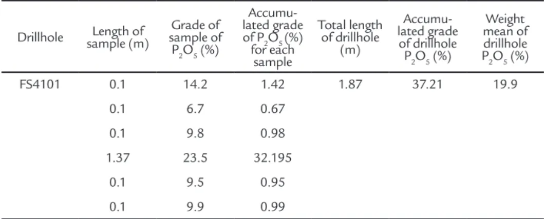
An accumulation process for trans-forming a set of 3D data to a 2D data set is divided into two steps. In the irst step, for each sample, the chemical variable is multiplied by its length, as in Equation 1.
(1)
where:
•
Z
ci = accumulated sample value;
•
Z
i= grade of the sample;•
L
i= length of the sample. In the second step, the sum of theac-cumulations is divided by the total length
after providing the weighted mean grade of the drillhole. At the end of the process,
there is a set of 2D data. A simple example illustrates the procedure – see Table 3.
Table 3
Example of the accumulation process used in this study.
Drillhole sample (m)Length of sample of Grade of P2O5 (%)
Accumu-lated grade of P2O5 (%) for each
sample
Total length of drillhole
(m)
Accumu-lated grade of drillhole P2O5 (%)
Weight mean of drillhole P2O5 (%)
FS4101 0.1 14.2 1.42 1.87 37.21 19.9
0.1 6.7 0.67
0.1 9.8 0.98
1.37 23.5 32.195
0.1 9.5 0.95
0.1 9.9 0.99
Z
ci
= Z
i+ L
ii= 1,2,...,n
Length ofdrillhole (m) drillhole PGrade of 2O5 (%) Arithmetic mean P2O5 (%) Weight mean P2O5 (%) Relative error P2O5 (%)
0.67 12 14.33 15.25 6.03
0.67 13
1.34 18 Table 2
Summary statistics for the theoretical example of regularization by ore zone.
Table 2 summarizes the mean calculations ignoring the differences
in basis between samples, and com-pares them with results considering the
grades by thickness in the calculation of the mean.
Accumulation creates a new set of 2D data, where each value
repre-sents the grade of a drillhole from ac-cumulated survey data (multiplied by
435
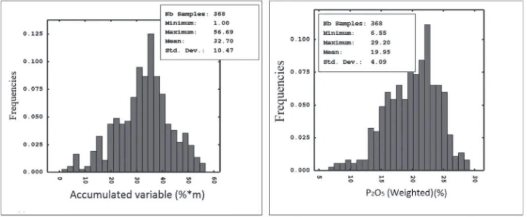
Figure 5 Histogram of (a) the accumulated variable and (b) the
variable of interest, the P2O5 layer.
To obtain a representative statistic for the deposit, an unbinding method was applied, namely the method of PoIygonal
Declustering (Isaaks and Srivastava, 1989). The weighted and declustering mean of the grades of P2O5 was 18.39%.
This mean grade will serve as a basis for validating the inal model, after the esti-mation process de-accumulation.
4.2. Structural analysis
The analysis of the spatial charac-teristics (similarity patterns) of region-alized variables relating to a mineral deposit is usually preceded by a criti-cal examination of the geology of the deposit and a full analysis of the data. There are several mathematical tools
to measure the spatial continuity of a mineral deposit, including madograms, covariograms, correlograms, etc. Stud-ies of autocorrelation in geostatistics are often referred to as variography because of traditional emphasis on the variogram or semivariogram (Sinclair
and Blackwell, 2002).
There is a strong anisotropy in the major directions of continuity (for both variables), as can be seen in the Figure 6. The result is summarized in Equation 2 and 3 (sph refers to a spherical shape).
Figure 6 (a) Directional variogram of variable thickness and
(b) directional variogram of the accumulated variable of P2O5.
Statistical analysis of the data is useful in helping to understand natural phenomena and especially the grades of the mineral deposits. Statistical analyses were performed with the accumulated data and the data was weighted. The weighted data was used as reference for validation of the inal results. For each survey, the
cumulative variable was divided by the length, resulting in a weighted average for the survey. This weighted variable (as it will be called from now on) is extremely important because it serves as a basis for the validation of the estimated model, as well as a reference for possible post-processing of the results (if necessary).
The layer of interest has 368 drill-holes with information on P2O5. Histo-grams with the accumulated data and weighted data on P2O5 can be seen in Figure 5 (a) and (b), respectively. Note that there are no multiple populations in the histo-grams, validating the geological model for this domain. Also, there are extreme values.
4. Results
4.1. Exploratory data analysis
in this study will be conducted using the accumulated variables (auxiliary variables) and the total length of
min-eralization in each drillhole. The grade of the variable of interest is obtained by an indirect method, which divides
the estimated auxiliary variable by the estimated thickness of the layer on the same node of the grid or block.
436 REM: R. Esc. Minas, Ouro Preto, 67(4), 431-437, oct. dec. | 2014
To estimate the accumulated P2O5 variable and the variable thickness, the ordinary kriging method was used (Matheron, 1963). The estimation was performed using a 2D block model. The blocks had X and Y dimensions of 50 m, and after the process of de-accumula-tion, had variable heights (Z-coordinates of the blocks in the geologic modeling procedure).
To perform the estimation by
ordinary kriging, the search ellipsoid was aligned with the variogram of the corresponding variable. A minimum of six and a maximum of 16 samples at a distance of 3000–2000 m in N135 and N45 were required. The search ellipsoid was divided into eight angular sectors. To avoid problems of de-accumulation after the estimates, it is important that the search strategy of the accumulated variable and the accumulator (in this
case, the thickness variable) is the same, and if necessary, the same variogram should be used for the estimation. In this case, it was possible to estimate each variable with its own variogram without further problems when mak-ing the de-accumulation. Figure 7 (a) shows the results of estimation for the variable thickness. Figure 7 (b) shows the estimation results for the cumulative variable P2O5.
(a) (b)
Figure 7
Location map with the results of the estimates for (a) variable thickness and (b) accumulated variable P2O5.
For each block of the estimated layer, the result of the accumulated vari-able P2O5 was divided by the estimated
value of the thickness. The results are shown in Figure 14 (b). A quick com-parison of the measured variable P2O5
(Figure 8 (a)) and the de-accumulated variable P2O5 (Figure 8 (b)) shows a good visual validation.
Figure 8
Location map of the (a) weighted variable of P2O5 (data) and (b) variable de-accu-mulation of P2O5.
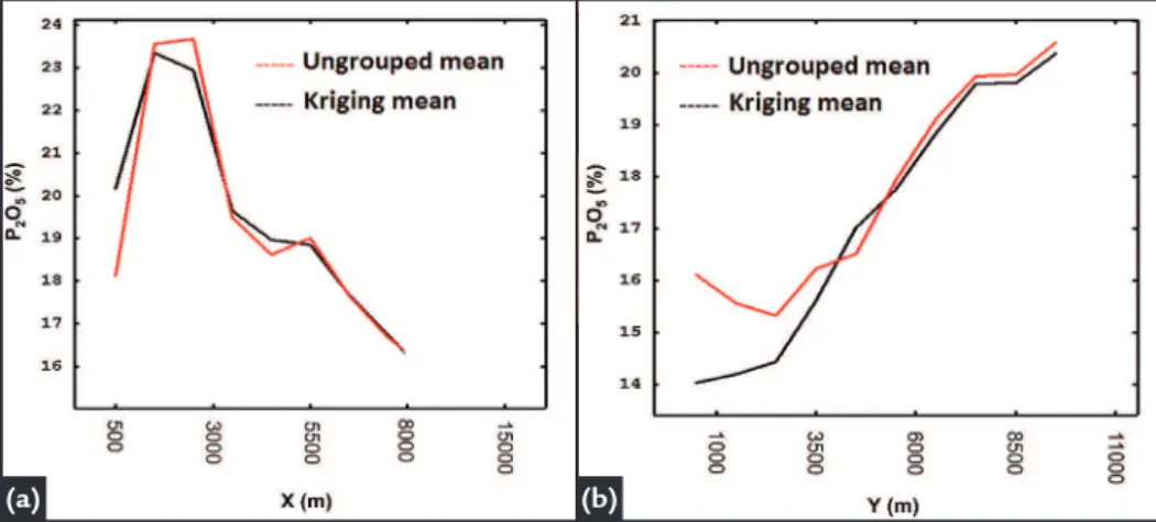
Besides visual validation, a valida-tion of the global mean was undertaken. The mean of the declustering weighted data was 18.39% and the estimate gave a result of 18.11% P2O5. Another way to validate the estimation is through the analysis of derivation (Swath Plot).
The analysis derivation performs a local validation, where the average block is compared with the average of the data in narrow bands in various directions of the block model. The validation was performed in two directions: along the east (slices every 500 m) and along the
north (slices every 500 m). The results can be seen in Figure 9 (a) and (b). In these igures, the red line represents the values read from ungrouped data by ‘nearest neighbor’ and the black line represents the values from the model obtained by kriging.
(a) (b)
4.3. Estimates
Importantly, both variables show the same directions of continuity, which
was expected. This does not mean that the direction of major continuity of variable
P2O5 is the same as that presented in the cu-mulative variable, although it is very likely.
(1)
437
Received: 12 September 2014 - Accepted: 25 October 2014. Estimates will only be adequate
if the initial data receives the correct treatment. The correction of the samples using regularization is essential to the practice of geostatistics, and the wrong choice of method can lead to a signiicant bias in the estimates. As demonstrated in this case study, the use of samples with different bases causes bias of the data mean.
Furthermore, regardless of the
adjustment of the sampling method, this bias can be propagated by spatial conti-nuity analysis, leading to inappropriate calculation of the weights of the samples in the estimation process.
As the case study with a stratiform deposit shows, with low thickness, there is the possibility of using unfolding tech-niques, a dynamic anisotropy search (in the estimate) and/or sub-blocks.
However, as no adequate basis
correction method was found to permit analysis of spatial continuity in 3D, these methods were discarded.
Although being an indirect es-timation method, the analysis and estimation of spatial continuity of the variables in 2D showed satis-factory results. Estimates made by this method require additional steps and more time to be realized than conventional estimates.
6. References
DEUTSCH, C. V. et al. Geostatistical reservoir modeling. New York: Oxford Univer-sity Press, 2002. 376p.
ISAAKS, E. H., SRIVASTAVA, M. R. An introduction to applied geostatistics. New York: Oxford University Press, 1989. 561p.
JOURNEL, A. G., HUIJBREGTS, C. J. Mining Geostatistics. London: Academic Press, 1978. 600p.
KOPPE, V.C., COSTA, J.F.C.L., KOPPE, J.C. Coordenadas cartesianas x coordena-das geológicas em geoestatística: aplicação à variável vagarosidade obtida por per-ilagem acústica. REM – Revista Escola de Minas, v. 59, n. 1, p. 25-30, 2006. KRIGE, D. G. Lognormal-de Wijsian Geostatistics for ore evaluation. Johannesburg:
SAIMM, 1981. 51p.
MARCOTTE, D., BOUCHER, A. The estimation of mineralized veins: a compara-tive study of direct and indirect approaches. Exploration and Mining Geology, v. 10. n. 3, p. 235-242, 2001.
MATHERON, G. Principles of geostatistics. Economic Geology, v. 58, p. 1246-1266, 1963.
MCARTHUR, G. J. Using geology to control geostatistics in the Hellyer Deposit. Mathematical Geology, v. 20, n. 4, p. 343-366, 1998.
SINCLAIR, A. J., BLACKWELL, G. H. Applied Mineral Inventory Estimation. Cambridge: Cambridge University Press, 2002. 381p.
5. Conclusions
(a) (b)
Figure 9 Analysis of drift (a) east and (b) north. The red line represents the contents ob-tained by ‘nearest neighbor’ (‘declustering