LONG-TERM PLANNING OF A CONTAINER TERMINAL UNDER DEMAND UNCERTAINTY AND ECONOMIES OF SCALE
Antonio G.N. Novaes
1*, Bernd Scholz-Reiter
2,
Vanina M. Durski Silva
1and Hobed Rosa
1Received November 3, 2010 / Accepted May 31, 2011
ABSTRACT.Governments of many developing countries are presently granting concessions to private organizations to operate container terminals. A key element in this process is the technical and economic evaluation of the project. In practice, the demand levels over time are volatile. The first part of the paper deals with a capacity expansion problem with stochastic demand. Next, an optimization model employs a dynamic programming routine to find the best epochs to install new berths. Ship waiting times are computed with queuing models and are introduced into the main model as upper restrictions based on international practice. Finally, a real options analysis is performed with the objective of evaluating the effects of an even-tual abandonment of the project at a pre-defined time horizon. The model is then applied to the container terminal of the Port of Rio Grande, Brazil.
Keywords: container terminals, capacity expansion, dynamic programming, abandon option.
1 INTRODUCTION
Governments in many developing countries traditionally regarded ports as national strategic assets which should remain under public control. However, in some cases container ports occasionally suffer from several critical problems that contribute to high logistics costs through-out the economy. These problems include equipment obsolescence, inefficiencies in labor devel-opment and labor allocation, lack of harbor capacity, and inefficiencies in the port administration model. Waiting times for berthing, on the other hand, are usually too high and yard space is often insufficient. In order to alleviate public investments normally scarce, it became common in developing countries the granting of concessions to private companies to operate port terminals. To give support to this operation, a crescent need for robust computer models intended to analyze port developments and their economic feasibility has been reflected in the literature.
*Corresponding author
1Federal University of Santa Catarina (UFSC), Florian´opolis, SC.
The optimization of logistics activities within maritime container terminals has attracted the attention of researchers and practitioners for more than forty years. Novaes & Frankel (1966) analyzed the generation process of unitized cargo (container, pallet, roll-on, roll-off) in a port and its relation to liner shipping, with the aid of a bulk queuing model. Taborga (1969), in his pioneering work on port planning, applied dynamic programming and queuing models to define the optimal epochs to add new berths to the terminal, and at same time choosing the best port technology with the objective of maximizing seaport returns. The economic appraisal of port in-vestments was analyzed by Goss (1967). Over the past recent years, the typical operating scheme of a container terminal has changed significantly. Larger container ships that call a modern port are often “classified ships” (Daganzo, 1990; Huanget al., 2007), in the sense that an appropriate berth slot is allocated to the vessel prior to its arrival. A non-classified ship, on the other hand, may have to wait until a berth of appropriate length becomes available to accommodate it. This means that the classical queuing models, that assume afirst-in,first-outservicing discipline, are no long adequate to represent this kind of port operation. New empirical approximate queuing approaches have been proposed to partially bypass this limitation (Huanget al., 2007; Morrison, 2007). In parallel, a number of researchers have relied on simulation techniques in order to plan resource utilization at a container terminal (Legato & Mazza, 2001; Kiaet al., 2002; Shabayek & Yeung, 2002), thus bypassing the queuing formulation drawback. But one serious limitation of the simulation approach in the context of developing countries is the lack of extensive and detailed data to be used in the models.
The use of containers for intercontinental maritime transport has dramatically increased around the world in the last decade (Notteboom, 2004). From about 150 million twenty-feet equivalent units (TEU) in 1996, the world container turnover has reached 496 million TEU in 2008. A further increase is expected in the upcoming years. Although the flow of containers in Brazil is approximately 1% of the world movement, the participation of containers in the country’s foreign trade has increased more than 11% a year in the period 1996-2008 (The World Bank, 2008). Brazil is following a trajectory of economic growth. Part of this growth is fueled by international trade, which is expected to continue to increase in line with Brazilian economic expansion. In such a scenario, port container terminals play an important role and represent a key asset of Brazil’s logistics system. In fact, the country has one of the longest coastlines in the world and the existence of container terminals in points of the Atlantic coast is an important advantage in international trade. However, in spite of this location advantage, the Brazilian port system suffers from some critical problems that contribute to high logistics costs throughout the economy. Among other limitations, the lack of harbor capacity, excessive ship waiting times, and inefficiencies in port administration are worth mentioning. Thus, improvements in port efficiency would have a major impact on reducing overall logistic costs.
and government policies (Daschkovska & Scholz-Reiter, 2009; G ¨unther & Kim, 2005; Kim & G¨unther, 2007). As a consequence, the forecasted demand levels tend to show a relatively high degree of uncertainty. The lack of reliable operational data, on the other hand, precludes in many cases the use of more detailed methods of analysis such as simulation techniques, for example. The objective of this paper is to present a robust, yet simple approach, to develop a long-term container terminal planning and evaluation model intended to analyze a port concession project in a developing country like Brazil. One characteristic of the methodology is the use of the basic data available in most developing countries. This paper is the improvement of the contents of two previous papers presented at academic conferences, namely Novaeset al. (2010a, 2010b). Although the analytical techniques used in this work are not new (capacity expansion modelling, queuing models to estimate waiting times, dynamic programming, real options), the contribution of the paper is essentially an integration of the techniques in one unique model framework, with the objective to solve practical problems of container port planning in developing countries, where the availability of data is often limited and the economic background is usually volatile. The paper is structured as follows: a mathematical formulation which allows for the introduction of demand uncertainty in the capacity expansion modelling is described in Section 2. A critical review of queuing model developments intended to estimate ship waiting times are analyzed in Section 3. The basic real option concepts and the application of the Black-Scholes equation (Smit & Trigeorgis, 2004) to an abandonment option are described in Section 4. TheTeconcontainer terminal of the Port of Rio Grande, Brazil, object of our application, is analyzed next in Section 5. The structure of the capacity expansion model is discussed in Section 6, including the description of a dynamic programming model used to minimize the net present value of berth investments, and its application to the case under analysis. In Section 7, the value of an abandonment option to be exercised at a pre-defined horizon during the project lifetime is estimated with the objective of improving its economical feasibility. Finally, conclusions are drawn in Section 8.
2 CAPACITY EXPANSION WITH DEMAND VOLATILITY
Capacity expansion is the process of adding facilities over time in order to satisfy rising demand (Manne, 1961; 1967). Capacity expansion decisions generally add up to a massive commitment of capital. The efficient investment of capital depends on making appropriate decisions in ex-pansion undertakings, in such a way the demand remains satisfied over an extended time period, with a minimum discounted lifespan cost. The literature shows, along the last forty years, an evolving sequence of capacity expansion models, starting with a simple deterministic and linear demand formulation (Manne, 1961), and extending it to non-linear, probabilistic demand situa-tions (Manne, 1967; Freidenfelds, 1980, 1981; Higle & Corrado, 1992; Beanet al., 1992; Novaes & Souza, 2005; Novaeset al., 2010a).
2.1 The cost function
The project will increase its own value by adopting the investment plan that minimizes N P V. The classicalN P V calculation presupposes that unknown-risk future monetary values are sum-marized by their expected values. Assuming no backlogs in demand are admitted, the net present value of investments, costs, and salvage value is
N P V =I0+ n
X
i=1
Iiexp(−r ti)− n
X
i=1
SVtiexp(−r t)+ T
Z
t=0
C(t)exp(−r t)dt (1)
where I0 is the investment at time t = 0, Ii is the value of the money inversion of orderi, (1≤i≤n),ris the annual continuous interest rate,ti is the time instant when the investmentIi is made,C(t)is the system operating cost at timet,T is the duration of the project, andSVti is
the salvage value of the project at timeT.
The cost functions associated with port operations reported in the literature vary slightly among authors (Huanget al., 2007). Usually these equations incorporate ship costs and berth operating costs in different forms. With regard to berth operating cost, we assume that it depends only on the demand level (throughput). In our approach, demand is an external variable, not depending on port servicing prices and service levels. Additionally, no demand backlog is admitted to occur, i.e. it is assumed that the port will provide adequate facilities before full congestion may occur. Consequently, the integral in the right hand side of expression (1) is constant in our capacity expansion model, and therefore does not affect the minimization of N P V. Thus, the capacity expansion model adopted in this application assumes only port investments and its salvage values, which reduces expression (1) to
N P V =I0+ n
X
i=1
Iiexp(−r ti)− n
X
i=1
SVtiexp(−r t) . (2)
Later, when analyzing cash flow and the abandon option, terminal operating costs and servicing prices will be introduced (see Section 7).
2.2 Economies of scale
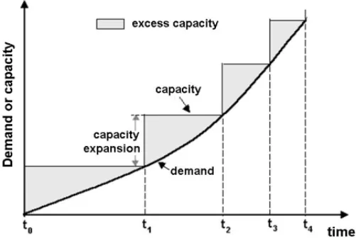
An important characteristic of most capacity problems is the recognition of economies of scale, i.e. large installations usually cost less per produced unit than small ones. But, if the demand level is continuously rising on the long run and demand backlogging is not permitted, excess capacity will occur (Fig. 1). Thus, there is a trade-off between scale economies and excess capacity cost, leading to a compromised optimal solution.
Figure 1– The classical capacity expansion process (Manne, 1961).
costs (including construction, administration, logistics, etc.) fall by a constant and predictable percentage. Mathematically the experience curve is described by a power law function
I(m)=I(1)m−θ (3) where I(1)is the value of the building cost of the first unit, I(m)is the value of the investment on themthunit, andθis the elasticity of building cost with regard to the number of units built in sequence. A experience curve that depicts a 25% cost reduction for every doubling of the number of built units is called a “75% experience curve” indicating that unit cost drops to 75% of its original level when installing the second item of the series, and so on. Letδbe the experience factor, obtained via (3) as
δ=I(2)
I(1)=2−θ (4) Applying logarithms to (4) one has
θ = −lnδ
ln 2 (5)
and the total investment related to the installation ofmunits in series is
I(m)=I(1) n
X
j=1
j−θ. (6)
Letmi be the number of berths to be installed simultaneously at time τi, and Ii(mi) the corre-sponding investment. To incorporate returns to scale in the analysis, we substitute variableI(mi)
i forIi in equation (1), thus adding the decision variablemi into the model.
2.3 Capacity expansion modelling 2.3.1 The linear expansion model
assumed that the facility has an infinite economic life and, whenever demand catches up with the existing capacity, xadditional unities of same capacity are installed. No backlog in demand is admitted. The objective is to determine the optimal capacity additionx, and the consequent time interval1T between increments. The time origin is the pointt0, followed by regeneration points att0+1T,t0+21T,t0+31T, that represent instants at which the previously existing excess capacity has just been wiped out. Note that when the system has reached t0+1T, the future looks identical with the way it appeared at timet0. The investment necessary to add a capacity increment of sizex, is assumed to be given by a relationship in the form of a power function, with economies of scale
I(x)=kxa, (k>0;0<a<1) . (7)
The demand, in this case, varies linearly over time and is expresseddt =μt, withμ > 0. The objective function to be minimized is of type (2). Let N P V(x)be a continuous function of xthat represents the sum of all discounted future investments looking forward from a point of regenerationt. We may write down the following recursive equation (Manne, 1961)
N P V(x)=kxa+e−r tN P V(x) . (8)
The first term on the right hand side of (8) represents the investment cost incurred at the begin-ning of the current cycle. Since it is assumed that the facilities have an infinite economic life, the salvage value of the project in this case is nil. The second term represents the sum of all installation costs incurred in subsequent cycles, discounted from the next point of regeneration back to instantt0, with a continuous interest rater. It follows directly that
N P V(x)= kx a
1−exp(−r t). (9)
But, sincet=x/μ, expression (9) becomes
N P V(x)= kx a
1−exp(−r x/μ). (10)
The optimal expansion size xˆ is obtained by minimizing N P V(x)with respect to x, and the optimal expansion time interval1t is given by1t = ˆx/μ(Manne, 1961, 1967). Manne (1961) extended his deterministic model to a stochastic demand formulation, with an underlying linear growing rateμand standard variationσ (Hull, 1997; Novaes & Souza, 2005). Such a model is based on Brownian motion theory, specifically the Bachelier-Wiener diffusion process in contin-uous time. One is interested in determining the instanttwhere demand first exceeds the installed capacity. At that time additional facilities will be supplied. In stochastic process terminology, one seeks the first passage time at point x, with probabilityu(t,x). The following difference equation applies to the problem (Manne, 1961; Novaes & Souza, 2005)
where p is the probability that one incremental step 1x is directed to increasing x, and q = 1− p is the probability that the step1x is directed to the opposite direction. Expand-ing expression (11) accordExpand-ing to Taylor’s theorem up to terms of second order, and dividExpand-ing both sides by1t, one gets
∂u(t,x)
∂t =(q−p)
1x
1t
∂u(t,x) ∂x +
(1x)2
21t
∂2u(t,x)
∂x2 (12)
The Laplace transform ofu(t,x)is
U(r,x)=
∞ Z
t=0
u(t,x)e−r tdt, (13)
wherer, in this formulation, is both the transformer parameter and the discount interest rate (Manne, 1961). Applying the Laplace transform to each side of (12), and recalling the boundary conditionu(0,x) = 0, one gets a second-order linear differential equation with respect to x. Its characteristic equation has two real roots
λ1= μ σ2
1+ s
1+2rσ 2
μ2
and λ2= μ σ2
1− s
1+2rσ 2
μ2
. (14)
After some transformations and simplifications (Manne, 1961), one gets
U(r,x)=eλ2x. (15)
Note thatλ2is a function ofμ,σ, andr, being independent of the quantityx. Sinceu(t,x)dt represents the probability with which exactlytyears have elapsed between two successive points of regeneration, the probability analogue of (8) is (Manne, 1961)
N P V(x)=kxa+
∞ Z
t=0
u(t,x)e−r tN P V(x)dt. (16)
Just as in the deterministic case, the first term on the right hand side of (16) is the present cost of installing a facility of capacity x. The second term of (16) is the probability that the next point of regeneration will occur int units of time, discounting the corresponding cost back to the present, and integrating over allt. Departing from (16), and recalling the basic definition of Laplace transform (13), one has (Manne, 1961)
N P V(x)
k = xa
1−U(r,x). (17)
Substituting (15) forU into (17), one has
N P V(x)= kx a
1−exp(λ2x)
From (14) it follows thatλ2<0 forμ >0, andr >0. Comparing (10) and (18), it is seen that the following equivalence holds (Beanet al., 1992)
r∗= −μλ2=
μ
σ
2
s
1+2r
σ
μ
2
−1
, (19)
meaning the linear stochastic model can be solved through an equivalent deterministic model in which the original discount rater is substituted by the modified rater∗ (Srinivasan, 1967; Freidenfelds, 1980; Beanet al., 1992; Higle & Corrado, 1992). Manne (1961) indicated that, in the deterministic model, the optimal expansion sizexˆincreases as the discount rateris lowered. For the probabilistic model, Manne (1961) showed that the greater the variance σ2, the lower will be the value ofr∗, and the higher will be the optimal valuex.ˆ
2.3.2 Generalization to non-linear demand cases
Assume now thatd(t), the demand for product or service, is a semi-Markov process{d(t),t ≥0} (Beanet al., 1992). One is interested in selecting a sequence of capacity expansions to satisfy the demandd(t)over an infinite horizon at minimum expected discounted cost using a contin-uous interest rater. A continuous semi-Markov process{d(t),t ≥0}is said to be transformed Brownian motion with underlying rateμand standard variationσ if there exists a non-negative increasing deterministic transformation h such that d(t) = h(d(t)), where{d(t),t ≥ 0}is (linear) Brownian motion with drift μ > 0 and volatilityσ > 0. The functionh is referred to as the transforming function. Bean et al. (1992) demonstrated that if{h(d(t)),t ≥ 0}is a transformed Brownian motion as defined above, the interest rate r∗ to be used in the equival-ent deterministic problem is given by the same expression (19) obtained by Manne (1961) for demand following an ordinary (linear) Brownian motion. In other words,r∗ is independent of the transformationh. In more general terms, Beanet al. (1992) demonstrated that a stochastic capacity expansion problem may be solved via a deterministic problem formulation in which (a) the random expansion epochsτ (x)are replaced by their expected values; and (b) the original continuous discount factorris replaced by its equivalent valuer∗given by (19). In general terms, capacity expansion models with general cost structures and with demand based on a transformed Brownian motion can be solved with the equivalent deterministic problem and the equivalent discount factor (Beanet al., 1992).
2.3.3 First passage time
The Laplace transform of the probability distributionu(t,x), given by (15), allows to compute the expected value and the variance of the first passage time to the levelx. One has (Novaes & Souza, 2005)
E[τ] = −∂U(r,x) ∂r
r=0
and
var[τ] = −∂
2U(r,x)
∂r2
r=0
− {E[τ]}2= xσ 2
μ3 =
σ
μ
2
E[τ]. (21)
For the general case withd(t)=h(d(t))one has (Novaes & Souza, 2005)
E[τ] = h(x)
μ and var[τ] =
σ μ
2
E[τ]. (22)
3 QUEUING APPROXIMATIONS FOR CONTAINER PORT PLANNING
Researchers and practitioners have applied queuing models to port planning for more than forty years (Novaes & Frankel, 1966; Taborga, 1969; Noritake, 1978; Noritake & Kimura, 1983; Huang & Wu, 2005; Huanget al., 2007). The first papers dealt with general cargo operations and no product specialization, with the berthing process represented by aM/M/cqueue in Kendall’s notation (Page, 1972), and with afirst-come,first-serveddiscipline. Novaes & Frankel (1966) utilized bulk queues in their research work, but the objective of the analysis was not to compute ship waiting times, but to analyze the cargo generating process at the port. Along the years, the handling of cargo at ports became more and more specialized. As a consequence, the queue models that best fit the ship waiting time process have changed, with the Erlang Ek1/Ek2/c
and theM/Ek/cKendall types being the most commonly used in container terminal planning (Huanget al., 1995; Kozan, 1997; Huanget al., 2007). The Erlang distribution has the following probability density function
f(x)=λkxk−1e−λx(k−1)!, (t≥0,k=1,2, . . . ,∞) , (23)
wherexis the random variable under analysis,λis the mean arrival rate, andkis the order of the distribution. The Erlang distribution can be viewed as being composed bykphases, each phase formed by a negative exponential distribution with the same average length 1/λ. The parameter kis an integer, and fork=1 the distribution repeats the negative exponential distribution. The mean and the standard variation for the Erlang distribution (23) areE[x] =k/λandσx =√k/λ, respectively. In general, the Erlangian queue is represented byEk1/Ek2/c, where the interarrival times and service times are distributed according to Erlang distributions of order k1 and k2, respectively. Other queue models can also be treated mathematically. The reader is referred to Fogliatti & Mattos (2007).
3.1 Approximate methods
(Page, 1972). Expressing the mean waiting time as a fraction of the mean service time, Page’s interpolation formula is
q(Ek1/Ek2/c)∼= 1−v2
a
v2swq(D/M/c)+(1−v2s)va2w (M/D/c)
q +va2vs2w (M/M/c)
q (24)
whereq(Ek1/Ek2/c) is the relative waiting time for a E
k1/Ek2/cqueue, andq
(D/M/c),q(M/D/c) andq(M/M/c)are the relative waiting times for the queuesD/M/c,M/D/candM/M/c, respec-tively. In (24),va andvs are coefficients of variation of the inter-arrival time and of the service time distribution functions respectively, given by
va =σta
E[ta] and vs =σts
E[ts], (25)
wheretaandts are the ship inter-arrival time and the service time, respectively. For the Erlang queueEk1/Ek2/c, one hasva =1√k1andvs = 1√k2. Letλbe the mean ship arrival rate at the terminal and μthe mean service rate. Page (1972) presented numerical results in table format, which requires interpolation for intermediate values ofρ, the average berth utilization factor given byρ =λ/μc, which must be less than the unit to let the queue attain a steady state solution. Furthermore, Page’s tables are restricted toc≤10.
Another approximation, valid for the queueM/Ek/c, is (Cosmetatos, 1976; Huanget al., 2007)
Wq=
π0ρ(λ/μ)c λc!(1−ρ)2
(
1+k 2k +
1−1
k
(1−ρ)(c−1) √
4+5c−2 32ρc
)
, (26)
where π0is the probability of having no elements in the line waiting, according to a M/M/c queue. Recalling thatρ =(λ/μc),E[ts] =1/ts andq =W1/E[ts], substituting these expres-sions in (26), and making the necessary simplifications, one has the Cosmetatos’ formula
q = π0(ρc) c
cc!(1−ρ)2
(
1+k 2k +
1−1 k
(1−ρ)(c−1) √
4+5c−2 32ρc
)
, (27)
whereq is the mean waiting time expressed as a fraction of the mean service time. Since most of the main container terminals in the world show aM/Ek/cqueuing system, the above formula is extensively used in their planning process. Another approximate formula (Sakasegawa, 1976; Morrison, 2007), which is applied to the general queueG I/G/c, is defined as
q ∼= v 2 a+v2s
2
!
ρ−1+√2c+2
c(1−ρ)
!
. (28)
4 THE REAL OPTIONS APPROACH TO PROJECT EVALUATION
In basic terms, the classical discounted cash flow technique assumes that the organization will accept an investing alternative if the net present value of the project cash flow, computed with an appropriate discount rate, is positive. The calculation of the of the N P Vproject presupposes that unknown-risk future cash flows be summarized by their expected values. It is given by
N P V′ = − I0− n
X
i=1
Iiexp(−r ti)+ n
X
i=1
SVtiexp(−r T)
+ T
Z
0
R(t)−E(t)exp(−r t)dt,
(29)
where R(t)is the revenue of the project at timet and E(t)is the sum of all expenditures at timet, with the other variables having the same meaning as in (1). The project is accepted as economically feasible when N P V′ >0. In (29) ship waiting-time costs are not considered as expenditures since vessels belong to external organizations. Instead, constraints limiting ship waiting times are added to the model. These constraints are based on best maritime practices among leading container terminals of the world, in a benchmarking process.
4.1 A real options overview
It is widely recognized that the traditional discounted-cash flow approach to the appraisal of capital investment projects, such as the aboveN P Vrule, cannot properly capture management’s flexibility to adapt and revise later decisions in response to unexpected market developments (Trigeorgis, 1996). The value of an investment with options, on the other hand, is usually greater than the one obtained with the traditional approach because an option truncates possible losses at some point in time. In order to reduce possible negative effects, some measures are taken beforehand in order to limit losses to pre-defined values (Trigeorgis, 1996; Hull, 1997). Thus, one is able to withstand riskier situations, limiting losses to a bearable, pre-established level. In general, a firm’s ability to anticipate and to respond flexibly to such changes reduces its expected downside risk and thus lowers costs, and/or raises its revenues. In fact, flexibility adds value to most financial undertakings (Trigeorgis, 1996).
In addition to financial options (stock options, forwards, future contracts, etc.), the term real option refers to the extension of financial option theory to real, physical assets (Mun, 2002; Smit & Trigeorgis, 2004). The main categories of real options are growth options, the option to expand, the option to wait, the option to switch inputs, outputs, or processes, the option to reduce scale (downsizing), and the abandonment or exit option (Smit & Trigeorgis, 2004). Abandonment options are important in capital-intensive industries where management want to have the flexibility to capture some resale value for assets if their in-use value to the company falls (Novaes & Souza, 2005). This is the kind of real option that will be applied and discussed in this paper.
4.2 Valuing an abandonment real option
Basically, there are three general methods to solve real options problems: thepartial differential equation approach, the dynamic programmingapproach, and the simulation approach (Mun, 2002). The method employed in this paper, the Black and Scholes equation, belongs to the first group and is based on the Wiener-Ito process (Trigeorgis, 1996; Mun, 2002; Smit & Trigeorgis, 2004). Growth models of money-related variables generally presuppose that deviations are not linear, being expressed as a proportion (a percentage) of the asset value. Let S be a money-related variable for which we want to study the variation d S/S. One writes the corresponding Ito process equation (Hull, 1997)
d S
S =μdt+σd z or d S=μSdt+σSd z, (30) whereμSis the expected instantaneous growth rate,σ2is the volatility, andd zis a Wiener pro-cess (Hull, 1997). When (30) is observed, the valueSof the asset follows a log-normal process (Hull, 1997). Departing from equation (30), and considering a generic functionG of S andt, Ito derived a lemma that bears his name. Let Sbe the value of an asset such that the variable d S/Sfollows the Ito process. Assume that f is the price of an option or another derivative of the asset under consideration, with its value depending on S andt. Departing from Ito’s lemma and making substitutions and simplifications, the Black and Scholes differential equation is obtained (Hull, 1997)
∂f
∂t +rfS
∂f
∂S + 1 2σ
2S2∂2f
∂S2 =rf f (31)
where:
S = the present value of the asset;
f = the price of the derivative, which is a function ofS,t,randσ; rf = the risk-free interest rate.
Assume that demand grows stochastically and exponentially with an underlying growing rateμ
and standard variationη. The integration of (30), makingη = 0, yields the expected growth function ofS
where S0 is the value ofS att = 0. Considering the process evolution from instant t −1 to instantt, one has
S(t)=S(t−1)exp(ut) , (33) leading to
ut =ln[S(t)] −ln[S(t−1)]. (34)
Taking a time series containingn values ofut, one estimates its mean and standard deviation. The timetis usually measured in days, weeks, or months, so we have to compute the equivalent annual standard deviation in order to evaluate the volatilityσto be used in the calculations (Hull, 1997). It is interesting to observe that the Black-Scholes equation separates the risk-free return on the investment, represented byrf, from the risk generated by the market variability, expressed by its volatilityσ. For a European put option the boundary condition to solve (31) is (Hull, 1997)
put=max{X−S,0} for t =TA, (35)
whereXis the exercise price andTAis the time to expiration. The integration of (31), subject to (35), yields
put=Xexp(−rfTA)N{−d2} −S N{−d1}, (36) whereN{∙}is the cumulative unit normal probability distribution, with
d1
ln
S X
+(rf +0.5σ2)TA 1
σ√TA
and d2=d1−σ √
T. (37)
The value of a European call option is similarly determined assuming the appropriate boundary condition (Hull, 1997)
call=S N{d1} −Xexp(−rfTA)N{d2}. (38)
The Black-Scholes equation gives a way of computing the economic impact of a real option as, for example, the exiting or abandonment option. One way of obtaining the value of an abandon-ment option is to make the strike price X equal to the salvage value of the abandoning project at time TA, and the value of the underlying asset S equal to the present value of the project cash flow. The correspondingputoption is calculated with (36) and its value is added to the net present value of the project, improving its economic performance. It must be pointed out that the Black-Scholes equation formulation assumes normal distributions to represent stochas-tic variables. But random variables associated with demand in real options problems may show high kurtosis levels, contrary to the normal distribution which is not skewed. In the applica-tion to be described forth, the available data do not allow for kurtosis calculaapplica-tion, and thus the Black-Scholes equation gives, in fact, an approximate solution.
is retained, the expected value to be realized by the firm is S. Admitting that both X and S are lognormally distributed (Schnabel, 1992), Margrabe’s exchange option pricing model is (Margrabe, 1978)
f =X N{d1} −S N{d2}, (39) where X is the discounted value of the project asset when abandonment occurs and S is the discounted value of the project’s value-in-use (Schnabel, 1992). Here f is a call option on the abandonment value, and a put option on the project’s value-in-use (Margrabe, 1978; Schnabel, 1992). Margrabe (1978) shows that the option (39) is worth more alive than dead, which implies that its holder will not exercise it until the last possible moment. In other words, f is a European type option.
Letσpbe the volatility of the abandonment process. Margrabe (1978) decomposesσp2into two components,σX2andσS2, according to the following formula
σp2=σX2 −2σXσSρ+σS2, (40)
where σX is the volatility associated with the abandonment of the project,σS is the volatility associated with the value-in-use of the project, andρis the correlation between X andS (Mar-grabe, 1978; Schnabel, 1992). IfσX = 0, Margrabe’s model reduces itself to the Black and Scholes original abandonment option formulation. Since in practical applications the abandon-ment value is not deterministic (i.e.,σX >0), the use of Margrabe’s model is of advantage when analyzing abandonment options. The value of the option f, if positive, is added to the net present valueN P V′, given by (29), improving the economic performance of the project. If f ≤0, the abandonment scheme is not economically feasible, and therefore must be discarded or modified. The employment of the Black-Scholes equation to compute the economic impact of an abandon-ment option such as the one analyzed in this paper is not free from criticism.
5 THETECONCONTAINER TERMINAL
5.1 An overview of the terminal
In order to illustrate the practical application of the methodology to a container port terminal located in a developing country, we have used operational information obtained from the Port of Rio Grande, located in the south of Brazil. Its container terminal –Tecon– is operated on a 24-hour/day basis by a private company, Wilson and Sons, since 1997, under a 25-year concession period, renewable for an equal time, and granted by the Brazilian Government. The concession is of the “landlord port” type, in which the domain of the port authority is restricted to the provision of the infrastructure, while investment in the superstructure and terminal operation is the responsibility of the licensed private company (Cullinaneet al., 2005; Cullinane & Song, 2002).
continue to go up in line with Brazilian economic expansion. Brazil’s exports by value and by volume have grown significantly during the last thirty years. More importantly, the data indicates that export value has increased more rapidly than export volume. For example, the index of manufactured goods by value, increased almost 23-fold over the period examined. The volume of these exports, however, increased only about 12-fold over the same period of time. Overall, the value of total exports grew 50% more than their volume. Thus, the opportunity cost of marginal time spent in logistics activities has become higher. In this context, time, reliability, just-in-time delivery, and security are critical considerations now. Therefore, the ability to trade with other countries and to grow competitively will be increasingly intertwined with the country logistics system (The World Bank, 2008).
In this context, ports are a key asset in Brazil’s logistics context, serving the entire coastline, one of the longest in the world. However, in spite of the locational advantage, the port system suffers from several critical problems that impair its development and contribute to high logistics costs throughout the economy. These include equipment obsolescence, inefficiencies in labor devel-opment and labor allocation, lack of harbor capacity, and inefficiencies in port administration. Waiting times for berthing are too high and yard space is insufficient in several ports (The World Bank, 2008). Thus, the employment of robust and up-to-date techniques to analyze terminal expansions and its economic evaluation can lead to better port performance, promoting higher efficiency and competition.
The main products exported through theTeconare tobacco, thermoplastic resins, shoes, frozen poultry, furniture, leather, and auto-parts. Presently, the terminal has three berths, with a total extension of 850.0 m, and 12.5 m depth. Container ship waiting times are greater than the ones observed in other international leading ports of similar capacity. For instance, 33% of container ships that arrived in Rio Grande during 2008, waited more than 12 hours, and 14% waited more than 24 hours. These figures are similar to the results shown by the Port of Santos, the largest in the country, where 35% of ships waited more than 12 hours and more than half of these waited more than 24 hours in the same time period (The World Bank, 2008). In 2008, theTeconoperated 356,575 containers, equivalent to 598,196 TEUs.
5.2 Data analysis
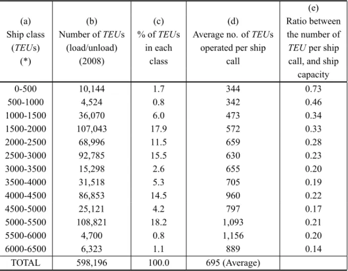
Although employing a good deal of real data in the analysis, obtained directly from the port administration, we have added some hypothetical variables in order to simulate the future de-velopment of the terminal. Table 1 shows the distribution of containers (both load and unload), and expressed in TEU among the various ship capacity classes, at theTecon in 2008. About 45% of the container flow was performed by ships in the capacity range 1500-3000 TEU. On the other hand, about 37% of the movement was done by Post-Panamax ships in the capacity range 4000-5500 TEU. In 2008, the average number of containers loaded/unloaded per ship call was approximately 695 TEU.
Table 1– Port of Rio GrandeTecon– container movement per ship class.
(a) (b) (c) (d)
(e)
Ship class Number ofTEUs % ofTEUs Average no. ofTEUs
Ratio between
(TEUs) (load/unload) in each operated per ship
the number of
(*) (2008) class call
TEUper ship call, and ship
capacity
0-500 10,144 1.7 344 0.73
500-1000 4,524 0.8 342 0.46
1000-1500 36,070 6.0 473 0.34
1500-2000 107,043 17.9 572 0.33
2000-2500 68,996 11.5 659 0.28
2500-3000 92,785 15.5 630 0.23
3000-3500 15,298 2.6 655 0.20
3500-4000 31,518 5.3 705 0.19
4000-4500 86,853 14.5 960 0.22
4500-5000 25,121 4.2 797 0.17
5000-5500 108,821 18.2 1,093 0.21
5500-6000 4,700 0.8 1,156 0.20
6000-6500 6,323 1.1 889 0.14
TOTAL 598,196 100.0 695 (Average)
(*) TEU: twenty-foot-long container equivalent unit.
However, when one analyzes the ratio between the number of TEUs operated per ship call, and the corresponding ship capacity, this index drops expressively with ship size. For instance, for ships in the range 5000-5500 TEU, the number of containers operated per ship call is only 21% of the ship capacity, while for vessels in the 500-1000 TEU range, the ratio is more than double that figure.
Another important index, considered when analyzing terminal productivity, is the average num-ber of containers loaded/unloaded per ship-hour. Letδ represent the fraction of forty-foot con-tainers on the total number of boxes. The berth productivity index, expressed as a number of containers transferred per hour, per ship (load/unload), can be estimated as
pr=(nTEU
1+σ )×
1 E
ts
, (41)
wherenTEU is the mean number of TEUs transferred per ship call (loaded/unloaded) and E[ts] is the average berth occupancy time. The variable did not vary significantly in the period 2001-2009, with a trend towardδ =0.70, value that has been adopted in the application.
On the other hand, E[ts]can be estimated as a function of nTEU, as depicted in Figure 2, and expressed approximately as
Figure 2– Relationship between the average berth occupancy time and the number of TEUs transferred per ship call.
It can been seen that there is a decreasing return to scale in terms of the time necessary to load/unload a ship, as a function ofnTEU. As a general rule, the container ships travelling south-bound in the Atlantic East Coast of South America stop in Santos and proceed directly to Buenos Aires, Argentina. In the way back, they stop in Montevideo (Uruguay), and next in Rio Grande. Thus, the vessels arrive atTeconwith a light load, generally carrying only the containers em-barked in Buenos Aires and Montevideo, plus the units to be discharged at the Tecon. One important characteristic of the Rio Grande’sTeconoperation observed in the last years is that the growth of demand is satisfied mostly by increasing the number of ship calls, instead of augment-ing the number of containers per stop. As a result, theTecondepth of 12.5 m is not a restriction today and probably not in the near future too, but it could be a severe constraint if the shipping lines substantially change their operating strategy such as, for instance, the establishment of a hub pole in Rio Grande (SCP, 2006).
Figure 3 shows the monthly evolution of theTeconthroughput from January 1999 to December 2009. Up to December 2003 the throughput (expressed in TEU) grew at an average rate of 21% a year. Due to the recent international crisis, theTeconthroughput evolution showed a downward inflection, but the trend is already changing, as seen in Figure 3. The volatility of the monthly series of throughput, from January 1999 to December 2009, is now computed. To do this (Hull, 1997) one converts these absolute monthly values D(t)= t = 0,1,2, . . .into relative returns u(t) = D(t)/D(t −1), t = 0.1,2, . . ., and then taking the natural logarithms, thus forming a series
Figure 3– Rio Grande’sTecon: Monthly throughput 1999-2009(TEU).
The coefficient of variation ofu(t)in the series is 0.201. Converting it to annual basis, one gets the demand volatilitycv=σ/μ=0.201√21=0.70, which will be used in our analysis. Ship inter-arrival times at the Teconare considered next. The analysis of 846 container ship arrivals in 2008 led to a mean inter-arrival time of 10.3 hours. Figure 4 shows the fitting result of a negative exponential distribution to the data. Ship service time, on the other hand, comprises the period of time the vessel effectively occupies a berth. Analyzing the same 2008 ship sample, the mean service time was 13.7 hours. An Erlang distribution withk =6 was fitted to the data, as shown in Figure 5. Although similar studies reported in the literature have indicated Erlang distributions of order 3 (Huanget al., 1995, 2007), theTeconresult can be justified by the shorter spread of the number of containers loaded/unloaded per ship call, as compared to other container ports around the world.
Figure 4– Ship inter-arrival time distribution.
Figure 5– Ship service time distribution.
6 TECON CAPACITY EXPANSION PLANNING
6.1 Model structure
respect-ing upper limits imposed by best maritime practices observed internationally. In Subsection 2.1, the following relation was defined
N P V =I0+ n
X
i=1
Iiexp(−rτi)− n
X
i=1
SVti exp(−r T) . (44)
In addition to the objective function (44) to be minimized, constraints limiting ship waiting time are added to the model. These constraints are based on best maritime practices among leading container terminals of the world, in a benchmarking process, but since the resulting improvement will not be instantaneous, their upper values are assumed to continuously decrease along time. Let Wq(t)be the maximum tolerable ship waiting time at instant t. Thus, the estimated ship waiting time at timetmust respect the constraint
Wq(t)≤W(t) . (45)
The berth loading/unloading productivity index is represented by the mean number of containers that are loaded/unloaded per ship, per hour. Considering a project lifetime ofT =25 years, we divided it into five-year periods, as indicated in Table 2, column (a). Column (b), of Table 2, shows the maximum ship expected capacity to be observed in each period. Column (c) shows the required berth length to receive ships with the capacities listed in column (b). Column (d) indicates the mean ship capacity in each epoch. Column (e) shows the expected numbernTEU of TEU operated per ship call in each time horizon. The mean berth occupancy time E[ts]is exhibited in column (f). Finally, the berth productivity index, represented by the mean number of containers loaded/unloaded per ship-hour, are shown in column (g). These figures are the expected coefficients to prevail during the lifetime of the project. The growth of the variable nTEU at theTeconwas assumed to follow a polynomial expression witht
nTEU(t)=695+19.11t+1.0036t2, (46) with t expressed in years. The values of nTEU computed via (46) for the time horizons of the project are exhibited in column (e), of Table 2. For each t, the value of nTEU(t)is com-puted. Thus, with (42), the variable E[ts]is estimated. Finally, the values of pr(t)are com-puted using expression (41). Column (g), of Table 2, depicts satisfactory berth productivity values to be respected along the lifetime of the project. In fact, the productivity of Tecon in 2003 was 21 containers/ship/hour (SCP, 2006), which has improved substantially during the last years, reaching about 30 containers/ship/hour in 2008. Thus, the productivity levels indicated in Table 2 represent, in fact, feasible targets, and were adopted in the optimization model.
6.2 The equivalent discount rate
Table 2– ExpectedTeconberth operating parameters per time horizon.
(a) (b)
(c) (d) (e) (f) (g)
Time Max. expected
Berth Mean ship nTEU
E[ts] pr(t)Berth horizon ship capacity
length (m) capacity (*) (hours) productivity
(years) (TEU) (TEU) (**) (***)
0-5 5500 280 3250 695 13.7 30
5-10 6000 300 3500 816 16.4 30
10-15 8000 340 4700 987 17.7 33
15-20 10000 360 6000 1207 19.3 37
20-25 12000 380 7100 1479 21.0 42
>25 14000 480 8300 1800 22.8 47
(*) Number of TEUs transferred per ship call; (**) average berth occupancy time per ship call; (***) containers/ship/hour.
of assets traded in the local economy. LetrˆM be the discrete average rate of return of such a portfolio. The risky assets contemplated by the investor have returns that are not known with certainty at the time the investments are made. TheCAPMasserts that the correct measure of risk of the asset is a coefficient calledbeta. The basic equation is
r′=r′f + ˆrM −r′f
β , (47)
wherer′is the expected rate of return,r′f is the risk-free rate of return, andβis a measure of the relative risk of the asset with reference to the whole portfolio (Campbellet al., 1997).
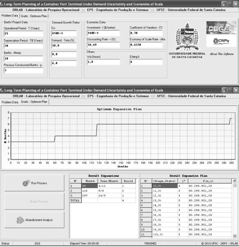
The risk-free return is the interest rate offered by entities that are entirely creditworthy during the period of a loan, such as the rates paid by the US Treasury and by some European government bonds. In theTeconapplication we have considered Brazilian figures, assumingr′f =0.036 or 3.6% a year,rˆM =0.10 andβ =1.2, leading tor′ =0.1128. The corresponding continuous-time discount rate isr = ln(1+r′)= 0.1069. The equivalent discount rate to be used in the model is given by (19), puttingσ/μ=cv=0.70, which is the volatility of the throughput series (Manne, 1961; Freidenfelds, 1981; Novaes & Souza, 2005). Applying (19) withr =0.1069, one hasr∗ =0.1048, value to be used in our analysis. As seen in Subsection 2.3.2, the impact of the stochastic behaviour of demand on the results is totally reflected by the discount rate reduction fromrtor∗(Higle & Corrado, 1992; Beanet al., 1992).
6.3 Investments on berth expansions
It is assumed, in the model, that the mean ship waiting time constraint (45) follows an expo-nentially decaying function, with Wq = 12 hours at timet = 0, reaching Wq = 2 hours at t =10 years, andWq=1 att =14 years, withWq=1 hour afterwards. In fact, due to budget restrictions, inefficiencies in port administration, lack of coordination between the terminal and shipping lines and cargo forwarders, among other factors, it is expected thatTeconperformance will not improve in a very short time period.
It was admitted that a berth investment is linearly depreciated in 30 years, with nil value at the end of its lifespan. Suppose a berth is installed at time t, with an investment It. The salvage value of the berth at the termination timeT of the project is (Fig. 6)
v=It
T
B−T+t TB
for t≤T and TB−T +t >0, (48)
withv=0 otherwise, whereTBis the berth depreciation time.
Time
= Salvage Value
Figure 6– Salvage valueSVof an investmentIt at timet.
6.4 The Dynamic Programming Algorithm
The dynamic programming concept has been broadly used in the literature to solve sequential decision problems of many kinds. Specifically, it can be used to optimize decision processes over time, which is the case of the problem treated in this paper. Dynamic Programming is, in essence, a general approach to optimization, rather than a mathematical algorithm as, for in-stance, the Simplex method used to solve linear programming problems. One essential feature of the dynamic programming approach is the reduction of a multivariate problem to a succession of single variable cases. At each stage of the optimization process the analysis of the resulting values of these single variables, with the appropriate decision rules, defines apolicy. The proce-dures of dynamic programming are based on thePrinciple of Optimalitydue to Richard Bellman: an optimal policy has the property that, whatever the initial state and the initial decision are, the remaining decisions must constitute an optimal policy with regard to the state resulting from the first decision (Bellman & Dreyfus, 1962).
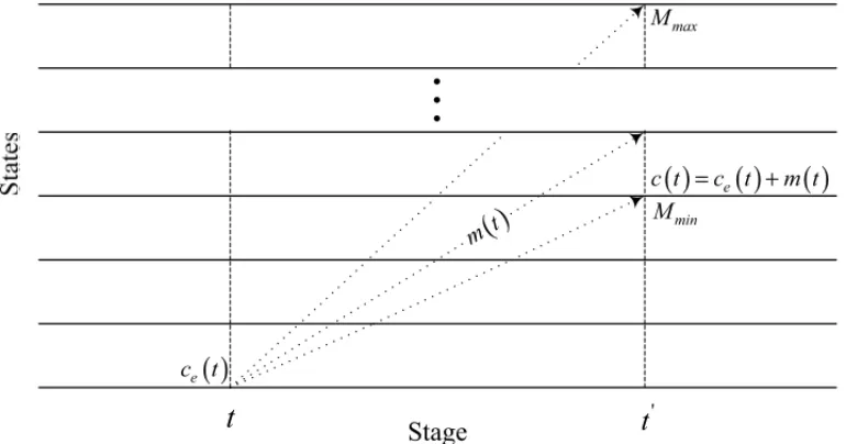
berths to the container terminal. The states of the process, on the other hand, represent the number of berths that will be available at staget, including the ones installed at previous stages plus the berths to be added at time t. At each stage of the process the minimum number of required berths Mmin is externally imposed in order to guarantee ρ(t) < 1, andWq(t) ≤ Wq(t). These restrictions help in reducing computational time, since the model investigates only feasible states. Thus, at each stage, the model first computes the minimum required number of berths. Letce(t) >0 be the number of berths already in operation at the beginning of stage t, and letm(t)be the quantity of berths to be added at that stage. The following procedure yields the value ofMmin:
Step 0: Initializece(t)and makem(t)←0.
Step 1: Makec(t)→ce(t)+m(t)and computeρ(t)=λ(t)[μ(t)c(t)]andWq(t)=q∙E[ts]. Step 2: Ifρ(t)≥1 orWq(t) >Wq(t), then makem(t)←m(t)+1 and go back to Step 1. Step 3: ReturnMmin←c(t).
Assuming the two operating restrictionsρ(t) <1 andWq(t)≤ Wq(t)are respected, the max-imum number of berths to be considered in the analysis is imposed by external considerations, mainly budget constraints and physical expansion limitations. In the former procedure the aver-age ship arrival rate is defined asλ(t)=D(t)
(360∙24∙nTEU)and the berth average servicing rate isμ(t) = 1/E[ts], wherenTEU is given by (46) and E[ts]by (42). All states that satisfy ρ(t) <1 andWq(t)≤Wq(t)are technically feasible, and therefore, can be evaluated according to the objective function (44).
The dynamic programming transitions from the generic staget1to the generic staget2are de-picted in Figure 7. In accordance to this evolving structure, the problem is solved in backward steps adopting the following algorithm (Hastings, 1973):
Step 0: Initialize the values ofce(0),Mmax, and other parameters of the problem. Step 1: Assign value zero to the terminal states.
Step 2: Repeat Steps 3, 4, 5 e 6 for each instantt.
Step 3: ComputeMminand repeat Steps 4, 5 e 6 for each feasible state.
Step 4: Repeat Steps 5 e 6 for each capacity expansion decisionm(t), until the maximum level Mmaxis reached.
Step 5: Compute the objective function value for decisionm(t), at the present staget. Step 6: If the present decision is better than the previous one, label it as temporary optimal. Step 7: Stop. Return the optimal capacity expansion sequence.
( )
'
( )
=( )
+( )
( )
Stage
Figure 7– Schematic evolution of the dynamic programming model.
limited to ten. Of course, in terms of dynamic programming this is a small size problem. When dealing with large problems it is possible that the classical dynamic programming approach be limited by dimensional restrictions. In such a case, approximate dynamic programming algo-rithms (Powell, 2007) can be used.
6.5 Capacity expansion results
Table 3– Optimal capacity expansion results.
Expansion date Number of berth Berth extension Investment value Year Month to be installed to be added (m) (US$ million)
4 11 1 280 67.2
9 8 2 2×300=600 126.0
24 9 1 380 81.6
Total 4 1,260 274.8
7 ECONOMIC FEASIBILITY ANALYSIS 7.1 The basic scenario
Suppose a private firm is negotiating, with the public port agency, the concession to operate the Tecon terminal for a period of 25 years. At the end of the concession period the government agency agrees to fully reimburse the private operator with a sum equal to the non-depreciated part of the investments made on berths and equipments, following the scheme indicated in Sub-section 6.3. The port agency also requires that the proponent pay a lump sum of 65 million dollars to the government at the signature of the contract.
The economic evaluation to be described next was performed considering the point of view of the proponent firm. Of course, a similar analysis should be performed by the public port agency, considering not only its own economic and financial objectives, but the social impacts as well. Such analysis is not done here due to lack of space and because it would involve considerations of quite different nature. In addition, if the private operator will decide to abandon the project at a certain date, it would mean that the market value of the project at that moment would perhaps not cover the non-depreciated part of the investments. Then, the government agency might not accept to reimburse the private operator to cover the non-depreciated part of the investments fully. But contractual clauses are binding and depend on other factors as, for example, public incentives to attract private investments, political strategies, etc. Of course, other contractual terms can be tested with this methodology, which is not done here due to space limitations. In order to compute the N P V′ value of the project, the prospective operator estimates a net margin of 11 dollars per transferred T EU. Thus, the value of R(t)−E(t)in relation (29) is simply 11×D(t), where D(t)is the throughput at timet, expressed in TEUs. The volatility
σpof the project is obtained with relation (40). The values ofσSandσX can be estimated by simulation. In this application, however, we assume hypothetical values due to space limitations. LetσS=0.70 be the volatility of the project’s value-in-use. With regard toσX, the abandonment option is composed by two parts: the present value of the cash flow accrued by the project during the period 0 < t ≤ TA and the present value of the salvage value to be accrued at time TA. The latter has a deterministic value in this application, since, under the contractual terms, the government accepts to pay a pre-defined amount of money to the private operator at the end of the deal. Thus, one hasσX < σS, sayσX = 0.40. The correlation betweenσX andσS was assumed to beρ=0.4, leading toσp=0.72.
In the sequel, the prospective operator analyzes the possibility of proposing an abandonment option to the port agency. The discounted value of the project asset abandonment value is
X = − I0+ iA
X
i=1
Iiexp(−rfti)+ TA
Z
t=0
[R(t)−E(t)]exp(−rft)dt
+ ϕX iA
X
i=1
SVtiexp(−rfTa), such that ti ≤TA,
(49)
where 0≤ ϕX ≤1 is a reducing factor to be applied to the salvage value, andiAindicates the order of the last investment such thatti A ≤TA. The prospective operator will try to increase the value ofϕ, while the port agency will argue in the opposite direction. In fact, the state agency wants to discourage an early abandonment of the project by reducing the value ofϕX as much as possible. At the end of the discussion, both parties agree to setφX =0.8. The discounted value of the project’s value-in-use, on the other hand, is
S = − I0+ n
X
i=iA+1
Iiexp(−rfti)+ T
Z
t=TA
[R(t)−E(t)]exp(−rft)dt
+ n
X
i=iA+1
SVtiexp(−rfT), such that ti >TA.
(50)
Now, the whole salvage value of the project will be reimbursed to the private operator, as agreed, covering the non-depreciated part of the investments at timeT.
The prospective operator tried different values of TA, but the project remained infeasible for TA <17 years. For TA = 17 years andrf =0.05827 (equivalent tor′f = 0.06 discrete dis-count rate), the Margrabe model producedS=91.21 million and X =30.29 million. Applying relation (39) withσp = 0.72 and the above values of S and X, one gets f = 17.21 million, which is the value of the put/call option according to Margrabe’s method. Finally, the modified net present value of the project is equal toN P V′ = −0.43+17.21 =16.77 million (Fig. 9). WithTA =17 years the project is feasible now, and the project should be submitted to a sensi-tivity analysis before it is presented to the port agency for further discussion and approval.
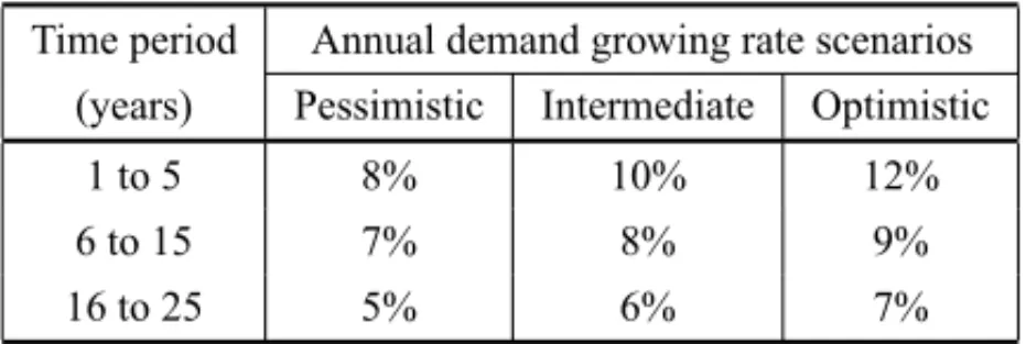
7.2 Sensitivity analysis
Figure 9– The abandonment option economic result.
Table 4– Demand forecasting curves.
Time period Annual demand growing rate scenarios (years) Pessimistic Intermediate Optimistic
1 to 5 8% 10% 12%
6 to 15 7% 8% 9%
16 to 25 5% 6% 7%
two berths implemented simultaneously, as depicted in Table 3 for the “intermediate” situation. For the “pessimistic” growth pattern no return to scale was registered. The same financing criteria adopted for the “intermediate” demand growing pattern has been applied to the “pessimistic” and “optimistic” cases. As expected, the latter produced better N P V′result, but the “pessimistic” case showed a negative N P V′ value. If the lump sum to be paid to the port agency would be reduced from 65 million dollars to 60 million, with all the other conditions unchanged, the project would be feasible for the three demand pattern scenarios. The economic result obtained forδ=0.80, on the other hand, although smaller when compared with theδ=0.75 scenario due to the inexistence of returns to scale, repeated the same scheme, with the “pessimistic” pattern requiring a 5 million dollars reduction in the lump sum payment. Changing fromδ =0.80 to
δ =0.85, the results were the same since no returns to scale were incorporated into the model. Thus, in order to have a positive result for the three alternative scenarios depicted in Table 4, the prospective operator could argue to get a reduction of 5 million dollars in the down payment, maintaining all the other factors defined in Subsection 7.1 unchanged.
8 CONCLUSIONS
it economically feasible. Most part of the data was obtained from theTeconcontainer termi-nal, Port of Rio Grande, Brazil. In developing countries like Brazil, the port operational data is usually incomplete, and therefore the planning of future operations and marketing strategies are limited. On the other hand, the allocation of funds for expansions and maintenance heavily depends on political factors. With the growing trend to transfer at least part of port operations to private organizations, it becomes necessary to evaluate in more detail the economic perspec-tives of such endeavours, even considering data limitations and other restrictions. Thus, a model framework as the one presented in this paper, even with its limitations, can help the parties in the process of getting a satisfactory agreement.
ACKNOWLEDGMENTS
This research has been supported by the Brazilian CNPq/Fapesc/Pronex Project no. 1.0810-00684 and by Capes/German Research Foundation (DFG), Bragecrim Project no. 2009-2.
REFERENCES
[1] BEANJC, HIGLEJL & SMITHRL. 1992. Capacity expansion under stochastic demands.Operations Research,40(2): S210–S216.
[2] BELLMANR & DREYFUSSE. 1962.Applied Dynamic Programming.Princeton University Press, Princeton, New Jersey.
[3] CAMPBELLJH, LOAW & MACKINLAYAC. 1997.The Econometrics of Financial Markets. Prince-ton University Press, PrincePrince-ton, New Jersey.
[4] COSMETATOSGP. 1976. Some approximate equilibrium results for the multi-server queue (M/G/r).
Operational Research Quartely,27: 615–620.
[5] COUTOJP & TEIXEIRA JC. 2005. Using linear model for learning curve effect on highrise floor construction.Construction Management and Economics,23: 355–364.
[6] CULLINANEK & SONGDW. 2002. Port privatization policy and practice.Transport Reviews,22(1): 55–75.
[7] CULLINANEK, JIP & WANGT. 2005. The relationship between privatization and DEA estimates of efficiency in the container port industry.Journal of Economics and Business,57: 433–462.
[8] DAGANZO CF. 1990. The productivity of multipurpose seaport terminals.Transportation Science,
24(3): 205–216.
[9] DASCHKOVSKAK & SCHOLZ-REITERB. 2009. How can electronic seals contribute to the efficiency of global container system?Proceedings Second International Conference on Dynamics in Logistics – LDIC 2009, 144-53, Bremen, Germany.
[10] FOGLIATTIMC & MATTOS NMC. 2007. Queuing Theory.Editora Interciˆencia, Rio de Janeiro (in Portuguese).
[12] FREIDENFELDSJ. 1981.Capacity Expansion: Analysis of Simple Models with Applications. North-Holland, New York.
[13] GOSS RO. 1967. Towards an economic appraisal of port investments. Journal of Transport Eco-nomics and Policy, September, 1967, 249–271.
[14] G ¨UNTHERHO & KIMKH. 2005.Container Terminals and Automated Transport Systems.Springer, Berlin – Heidelberg.
[15] HASTINGS NAJ. 1973.Dynamic Programming with Management Applications. London: Butter-worths, London.
[16] HIGLE JL & CORRADOCJ. 1992. Economic investment times for capacity expansion problems.
European Journal of Operational Research,59: 288–293.
[17] HUANG WC, CHISAKI T & LIG. 1995. A study on the container port planning by using cost function with IND based on system.Journal of the Eastern Asia Society for Transportation Studies,
1: 263–276.
[18] HUANGWC & WUSC. 2005. The estimation of the initial number of berths in a port system based on cost-function.Journal of Marine Science and Technology,13(1): 35–45.
[19] HUANGWC, KUOTC & WUSC. 2007. A comparison of analytical methods and simulation for container terminal planning.Journal of Chinese Institute of Industrial Engineers,24(3): 200–209.
[20] HULLJC. 1997.Options, Futures, and Other Derivatives.Prentice-Hall, Upper Saddle River, New Jersey.
[21] KIA M, SHAYAN E & GHOTBF. 2002. Investigation of port capacity under a new approach by computer simulation.Computers & Industrial Engineering,42: 533–540.
[22] KIM K & G ¨UNTHER HO. 2007. Container Terminals and Cargo Systems. Springer, Berlin-Heidelberg.
[23] KOZAN E. 1997. Comparison of analytical and simulation planning models of seaport container terminals.Transportation Planning and Technology,20: 235–248.
[24] LEGATOP & MAZZARM. 2001. Berth planning and resources optimization at a container terminal via discrete event simulation.European Journal of Operational Research,133: 537–547.
[25] MANNEAS. 1961. Capacity Expansion and Probabilistic Growth.Econometrica,29: 632–649.
[26] MANNEAS. 1967. Investments for Capacity Expansion: Size, Location and Time-Phasing. Allen and Unwin, London.
[27] MARGRABE W. 1978. The value of an option to exchange one asset for another.The Journal of Finance,XXXIII(1): 177–186.
[28] MORRISONJR. 2007. Practical extensions to cycle time approximations for the G/G/m-queue with applications.IEEE Transactions on Automation Science and Engineering,4(4): 525–532.
[29] MUNJ. 2002.Real options analysis.Wiley, Hoboken, New Jersey.
[30] NORITAKE M. 1978. A study on optimum number of berths in public wharf. Proceedings of the Japanese Society of Civil Engineers,278: 113–122.