AN ANALYSIS OF TAGUCHI’S ON-LINE QUALITY MONITORING PROCEDURE FOR VARIABLES BASED ON THE RESULTS OF A SEQUENCE OF INSPECTIONS
Linda Lee Ho
1*and Roberto Quinino
2Received March 11, 2010 / Accepted November 12, 2011
ABSTRACT.In this paper, a procedure for the on-line process control of variables is proposed. This procedure consists of inspecting them-th item from everymproduced items and deciding, at each inspec-tion, whether the process is out-of-control. Two sets of limits, warning(µ0±W)and control(µ0±C), are used. If the value of the monitored statistic falls beyond the control limits or if a sequence ofhobservations falls between the warning limits and the control limits, the production is stopped for adjustment; otherwise, production goes on. The properties of an ergodic Markov chain are used to obtain an expression for the average cost per item. The parameters (the sampling intervalm, the widths of the warning, the control limitsW andC(W ≤ C), and the sequence length(h)are optimized by minimizing the cost function. A numerical example illustrates the proposed procedure.
Keywords: on-line process control, quality control by variables, Markov chain, warning limit, sequence of inspections.
1 INTRODUCTION
Taguchiet al. (1985, 1989) proposed an economical procedure to monitor on-line process con-trol with attributes as well as variables. This inspection system is automatic and allows for the sampling of only a single item at a time. In general, the proposed system can be implemented in high-speed electronics manufacturing facilities, where the testing equipment is connected to a central computer where data are taken automatically as the items that are produced are tested.
The procedure of on-line control for use in monitoring processes has been studied by many authors, such as Adams & Woodall (1989), Nayebpour & Woodall (1993), Srivastava & Wu (1991, 1995), Gong & Tang (1997), Borgeset al.(2001), Wang & Yue (2001), Dasgupta (2003), Trindadeet al. (2007), Dasgupta & Mandal (2008), Hoet al. (2007), Trindadeet al. (2007) and Quininoet al. (2010). Ho & Trindade (2009) presented a revision related to this topic and proposed an economical X control chart model for short-run production.
*Corresponding author
In Taguchi’s approach [Taguchiet al.(1989, 2004)], initially the process mean isµ=µ0(state I). At a random time, the process mean may shift from µ = µ0toµ = µ1 > µ0(state II). To control the quality of the process, after every m items have been produced, them-th item is examined. If the value of the quality characteristic does not satisfy the control limit, then production is stopped for adjustment. However, Taguchi et al. (1989; 2004) did not assume explicitly a probability function for the shift of the process mean fromµ =µ0toµ = µ1 >
µ0, and many simplifications and approximations were used to calculate the average cost per produced item and the optimum values of the sampling intervalm(hereafter denoted asm◦) and the width of the control limitC.
Adams & Woodall (1989) argued the inadequacy of Taguchi’s model and presented alternative procedures for random walk models. The optimum sampling interval and control limits obtained by direct search are presented in tables. Srivastava & Wu (1991, 1995) presented a second order approximation for Taguchi’s loss function and therefore presented closed expressions for the optimum sampling interval and control limits were also yielded.
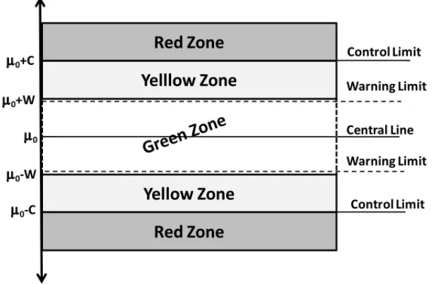
Traditionally, three horizontal lines are used to draw the standard (Shewhart) control charts: a central line (representing the average value of the quality characteristic at an in-control state) and two other horizontal lines, called the control limits (upper and lower). However, some analysts may suggest two sets of limits. The outer limits are the usual action limits and are called control limits (CL) (points that plot outside of this limit lead to a stoppage for an assignable cause) and the inner limits are called warning limits (WL). Points that fall between the warning limits and the control limits may cause suspicion that the process may not be operating properly. One may also suggest for an additional rule, similar to the additional rules described in the Western Electric Handbook (1956) to decide if the production process is in-control or not. Such additional rules are usually based on the sequence of the results of last inspections.
The purpose of this paper is to present a procedure for on-line process control by adding alter-native criteria that lead to an interruption of the production process not included in the previous listed papers. As in Taguchi’s approach, them-th item is inspected at everymproduced items. If the value of the monitored statistic falls beyond the control limits (red zone – RZ) or a sequence of h observations falls between the warning limits and the control limits (yellow zone – YZ), then the production is stopped for adjustment; otherwise, (green zone – GZ) production goes on. The parametersh,C,W and m are determined such that they minimize the average cost per item of the controlled system. Figure 1 represents schematically the new proposal.
Figure 1– Schematic representation of the inspection system.
obtained by Hoet al.(2007) is successful. This paper is organized as follows: Section 2 describes the probabilistic inspection model. In Section 3, an economic model is developed to determine the optimum designs. In Section 4, a numerical example illustrates the proposed model. The conclusions are presented in Section 5.
2 PROBABILISTIC MODEL
Consider a process that produces items and a quality characteristic of interest(X)that can be described by a Normal distribution with meanµand standard deviationσ. The process starts in-control, in other words, its process mean isµ = µ0(State I), and the process may shift to
µ =µ1,µ1 6=µ0. The duration of the process in-control condition is usually modeled by an exponential distribution for a continuous case. The geometric distribution behaves similarly to the exponential distribution, but it is typically used for the discrete case in which the duration is measured by the number of units that are produced before the shift. Following previous papers [Nayebpour & Woodall (1993), Nandi & Sreehari (1999), Jiang & Tsui (2000), Borgeset al.
Both the geometric and exponential distributions are memoryless, which facilitates mathemati-cal analysis. However, these distributions are useful for other reasons than their mathematimathemati-cal facility. Many researchers have recently used exponential or geometric distributions to describe shifts from in-control to out-of-control states. For example, Wang & Sheu (2003), Zhanget al.
(2008), Serel & Moskowistz (2008), and Lim & Cho (2009) employed exponential distributions, but Hoet al. (2007), Trindadeet al. (2007), Dasgupta (2008) and Ding & Gong (2008) used geometric distributions. Such distributions not only facilitate the development of mathematical models but also allow application to real problems, as mentioned in the cited papers.
Three horizontal lines are used to build standard (Shewhart) control charts, one drawn atµ=µ0 and two others atµ0±C(upper and lower control limits (CL)). However, one may suggest two sets of limits; the outer limits are the usual action limits (CL), and the inner limits are drawn at
µ0±W,W ≤C. To illustrate these limits (see Fig. 2), one may use different colors to identify the different zones. Points that plot outside of the control limits lead to a stoppage for an assignable cause (red zone); points that fall between the warning limits and the control limits may reveal that the process may not be operating adequately (yellow zone); otherwise, the pro-cess must operate adequately if the points fall between the warning limits (green zone).
µ
µ
µ µ
µ
Figure 2– Warning and control limits.
Let Xi,i =1,2,3, . . . ,∞, denote the observed values of some characteristic of interest at the
process mean has shifted toµ=µ1, and all of the items in the current inspection are produced atµ=µ1. The second indexkis related to the result of the inspection:
• k = −1, the observed value of the current inspection is in the red zone (xi > µ0+Cor
xi < µ0−C); the next inspection is only after a production ofmitems, and the process is stopped for adjustment;
• k=0, the observed value is in the green zone,(µ0−W ≤Xi ≤µ0+W)and the process is not adjusted;
• k =1, the observed value is in the yellow zone(µ0+W ≤ Xi < µ0+C orµ0−C <
Xi ≤µ0−W), but the value of the previous inspection was not in the yellow zone and the process is not adjusted;
• k =2, the observed value is in the yellow zone(µ0+W ≤ Xi < µ0+C orµ0−C <
Xi ≤µ0−W), like the previous inspection and the process is not adjusted;
• k =3, the observed value is in the yellow zone(µ0+W ≤ Xi < µ0+C orµ0−C <
Xi ≤µ0−W), like the two previous inspections and the process is not adjusted;
• . . .
• k =h, the observed value is in the yellow zone(µ0+W ≤ Xi < µ0+C orµ0−C <
Xi ≤µ0−W), like the(h−1)previous inspections; the process is adjusted.
Note that there is an adjustment only ifk = −1 or k =h. A total of 3(h+2)states of chain
(s,k)is used to describe the inspection process. The second index assumes integer values in the interval−1≤k≤h andk =t ≥0, which indicates a sequence oft inspected items for which the observed values are in the yellow zone. Before the probabilistic model, let us introduce the following notations:
G0 = P(µ0−W ≤ Xi ≤µ0+W|µ=µ0)
G1 = P(µ0−W ≤ Xi ≤µ0+W|µ=µ1)
Y0 = P(µ0+W ≤ Xi < µ0+C|µ=µ0)+P(µ0−C <Xi ≤µ0−W|µ=µ0)
Y1 = P(µ0+W ≤ Xi < µ0+C|µ=µ1)+P(µ0−C <Xi ≤µ0−W|µ=µ1)
R0 = P(Xi > µ0+C|µ=µ0)+P(Xi < µ0−C|µ=µ0)
R1 = P(Xi > µ0+C|µ=µ1)+P(Xi < µ0−C|µ=µ1)
The transition probabilities from state(s,k)at the moment of inspectionito state(s∗,k∗)at the moment of inspection(i+1)are elements of the matrixP
P=
A00 A01 A02 A10 A11 A12 A20 A21 A22
where Ass∗ denotes the matrix of transitory probabilities p(s,k)(s∗,k∗); s,s∗ = 0,1,2; k,
k∗ = −1,0, . . . ,h. The elements ofA00 are the transitory probabilities from states (0,k)to
states(0,k∗). That is, the process is in-control at thei-th inspection, and it also stays in-control at the(i+1)-th inspection. The non-null elements of the matrixA00are expressed in (2).
p(0,0)(0,−1)= p(0,−1)(0,−1)=p(0,h)(0,−1)= p(0,k)(0,−1)=qmR0
p(0,0)(0,0)= p(0,−1)(0,0)= p(0,h)(0,0)=p(0,k)(0,0)=qmG0
p(0,0)(0,1)= p(0,−1)(0,1)= p(0,h)(0,1)=p(0,k)(0,k+1)=qmY0
(2)
for 0<k<h, withqm =(1−π )m.
The elements ofA01 are the transition probabilities from states(0,k)to states(1,k∗). That is,
the process is in control at thei-th inspection, but the parameter shifts fromµ=µ0toµ=µ1. Thus, some items are produced atµ=µ0, and at least the inspected item is produced atµ=µ1. The non-null elements of the matrixA01are expressed in (3), as follows:
p(0,0)(1,−1)= p(0,−1)(1,−1)= p(0,h)(1,−1)=p(0,k)(1,−1)=(1−qm)R1
p(0,0)(1,0) =p(0,−1)(1,0) =p(0,h)(1,0)= p(0,k)(1,0)=(1−qm)G1
p(0,0)(1,1) =p(0,−1)(1,1) =p(0,h)(1,1)= p(0,k)(1,k+1)=(1−qm)Y1
(3)
for 0<k<h, withqm =(1−π )m.
The matrixA02is a null matrix;A10 =A20and their non-null elements are the transitory
prob-abilities withk = −1 orh. That is, the process is adjusted in the previous inspection, and it restarts in-control in the current inspection employing the sampling intervalm:
p(1,−1)(0,−1)= p(2,−1)(0,−1)= p(1,h)(0,−1)=p(2,k)(0,−1)=qmR0
p(1,−1)(0,0) =p(2,−1)(0,0) =p(1,h)(0,0)= p(2,h)(0,0)=qmG0
p(1,−1)(0,1) =p(2,−1)(0,1) =p(1,h)(0,1)= p(2,h)(0,1)=qmY0.
(4)
Similarly, the non-null elements ofA11 =A21are also transition probabilities withk = −1 or h. However, after the adjustment, the process restarts in-control, but the parameterµshifts in the current inspection. Thus, the non-null elements of these matrices are
p(1,−1)(1,−1) =p(2,−1)(1,−1)= p(1,h)(1,−1)= p(2,h)(1,−1)=(1−qm)R1
p(1,−1)(1,0)=p(2,−1)(1,0)=p(1,h)(1,0)= p(2,h)(1,0)=(1−qm)G1
p(1,−1)(1,1)=p(2,−1)(1,1)=p(1,h)(1,1)= p(2,h)(1,1)=(1−qm)Y1.
(5)
Next, we need the matricesA12andA22, which are the transition probabilities from states(1,k)
to states(2,k∗)and from states(2,k)to states(2,k∗), respectively. In these cases, the parameter shifted in the previous inspections, and the process has not been adjusted. A12 =A22 and the
non-null probabilities of these matrices are
p(1,k)(2,−1)= p(2,k)(2,−1)=R1
p(1,k)(2,0) =p(2,k)(2,0)=G1
p(1,k)(2,k+1)= p(2,k)(2,k+1)=Y1
for 0≤k <h. Note that the Markov chain built in this way incorporates information about the process (whether it is in-control or out-of-control), the length of the sequence of observations in the yellow zone and also the length of sampling intervalsmin the matrixP. MatrixPis ergodic recurrent and consequently1 = limu→∞Pu exists and does not depend on the probability of
the initial states of the process. Thus, all rows of 1are equal. By denoting the first row of the matrix1byδ =(δ(0,−1), . . . , δ(0,h), δ(1,−1), . . . , δ(1,h), δ(2,−1), . . . , δ(2,h))and solving the system of linear equationsδ=δPsubject to the restrictionP2
s=0
Ph
k=−1δ(s,k) =1,δ(s,k)can be determined. This solution can be interpreted as the proportion of inspections in state(s,k),
s=0,1,2;k= −1,0, . . . ,hover a large number of inspections.
3 COST FUNCTION
To obtain the cost function, more assumptions are needed. Once one decides to make an adjust-ment, the stoppage of the process is instantaneous. After the adjustadjust-ment, the process restarts at State I(µ=µ0). In this paper, the costs follow a structure similar to the usual economic designs, whereci is the cost for a single inspection andcais the cost for adjustment. In this paper, one item is stated as non-conforming if the observed value of the quality characteristic is beyond the specification limits(µ0±L E). Thus, the next costs related to non-conforming and discarded items are also included in the model: cn is the cost for delivering a non-conforming item (this item is sent to the customer or to the following production stage), andcDis the cost to discard the examined item. For each cycle of inspection, the(m−1)items are sent to the customer or to the following stages of production. It is assumed that all inspected items are discarded or rectified in the posterior stages once the inspection is partially destructive.
For a sufficiently large number of inspections,
δ= δ(0,−1), . . . , δ(0,h), δ(1,−1), . . . , δ(1,h), δ(2,−1), . . . , δ(2,h)
is the vector of the probability of the states of the Markov chain. LetCbe the random variables related to the cost at each cycle of inspection. We assume discrete values related to the states of the Markov chain. The cost of the state(s,k),s=0,1,2;k= −1,0, . . . ,hmay be written as
C(s,k) = ci +a(s,k)+n(s,k)+cD; s=0,1,2; k= −1, . . . ,h (7)
• ci,cD, respectively, are the costs to inspect and discard a single item, constants for all states(s,k),s=0,1,2;k= −1,0, . . . ,h;
• a(s,k)is the cost to adjust the process;
• n(s,k)is the cost to send non-conforming items to the customer or to later stages of the process.
In the next paragraphs, the different costs are detailed.
The cost for adjustment is included for states(s,k),s=0,1,2;k= −1,h. Thus,
a(s,k)=ca; s=0,1,2;k= −1,h.
• The cost to send non-conforming items to the customer or to later stages of the process:
For the states(0,k),k= −1,0, . . . ,h, all items are produced atµ=µ0; thus,
n(0,k)=cnp1(m−1);k= −1,0, . . . ,h,
withp1=1−P(µ0−L E ≤ Xi ≤ µ0+L E|µ =µ0). Similarly for the states(2,k), when all items are produced atµ=µ1, we have
n(2,k)=cnp2(m−1);
fork = −1,0, . . . ,h, with p2 =1−P(µ0−L E ≤ Xi ≤µ0+L E|µ =µ1). For the states(1,k),k= −1,0, . . . ,h,v <mitems are produced atµ=µ0, and then,m−vare produced atµ=µ1. Taking into account all possibilities
n(1,k)=cn
Pn
v=1π(1−π )v−1
(v−1)p1+(m−v)p2 1−(1−π )m
fork = −1,0, . . . ,h. For a large number of inspections and considering our setting as a renewal-reward process, the average cost per itemC E(m)is the ratio of the expected cost per inspection cycleE(V)by the quantity of items sent to the customer or to the following stages of production, expressed as
C E(m)= E(V)
m−1 =
P2
s=0
Ph
k=−1C(s,k)δ(s,k)
m−1 . (8)
Montgomery (2001) claimed that the economical design of the control chart must be evaluated jointly with some statistical criteria. He recommended strongly that the optimization of the cost function should be subject to an adequate statistical restriction. In this study, a set of additional restrictions are considered: a minimum value for the in-control average run length (A R L0)is denoted byφ0, and a maximum value for the average run length during an out-of-control condi-tion(A R Lε)is denoted byφ1. These values (φ0andφ1) are fixed as a part of the responsibility for the control system of the productive process.
The problem consists of determining the values of
m◦,W◦,C◦,h◦ = arg min (m,W,C,h)
[C E(m)]
subject to
(
A R L0≥φ0,
A R Lε ≤φ1
(9)
The values ofA R L0,A R Lεcan be calculated by employing the stationary vector
δ = δ(0,−1), δ(0,0), . . . , δ(0,h−1), δ(0,h), δ(1,−1), δ(1,0), . . . ,
δ(1,h−1), δ(1,h), δ(2,−1), δ(2,0), . . . , δ(2,h−1), δ(2,h)
and can be expressed as:
A R L0 =
δ
(0,−1)+δ(0,h)
δ(0,−1)+ ∙ ∙ ∙ +δ(0,h)
−1
;
A R Lε =
δ
(1,−1)+δ(1,h)+δ(2,−1)+δ(2,h)
δ(1,−1)+ ∙ ∙ ∙ +δ(1,h)+δ(2,−1)+ ∙ ∙ ∙ +δ(2,h)
−1
4 NUMERICAL EXAMPLES AND DISCUSSIONS
To illustrate the proposed procedure, consider the example adapted from Taguchiet al. (1989), Taguchiet al.(2004) and Trindadeet al.(2007).
A manufacturer of high-volume-integrated circuits wants to install a system to control the mea-surement of some dimension of interest. Historical data allows an estimation of the cost com-ponents asci = $0.25,cn = $20,cD = $2.0, andca = $900. The specification limits (LE) were fixed as±1.5, and the shifts from process in-control [State I(µ0 =0)] to out-of-control [State II(µ1 =1)] can be described by a geometric distribution with the parameterπ =0.001. The standard deviation of the process is known and is equal to 0.5. Managers responsible for the production system adoptφ0=370 andφ1=5 (minimum and maximum values for A R L0and
A R Lε, respectively). To calculate the optimum values, a program in MatLab was developed for this task. (Interested readers can request a copy of the program directly from the authors.)
Figure 3 shows the plots of the expected cost versus the sampling intervalm for some cases chosen to illustrate the behavior of the optimum set. The optimal design is as follows: The sampling interval ism0 = 27. The length of the sequence of observations in the yellow zone ish0 = 3. The width of the warning limit is W0 = 0.8, and the width of the control limit isC0 = 1.6; the results yield an average cost of $1.381. The current proposal is 4.4% less expensive when compared with the approach presented in Ho, Medeiros & Borges (2007). In that case, the sampling interval increases tom0=32 as the average cost also increases to $1.445 (withh =1 andW =C =1.4).
4.1 Sensitivity analysis
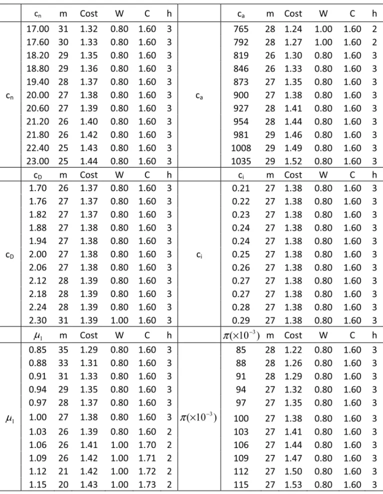
For the sensitivity analysis, each parameter is analyzed in a±15% range of values, and other parameters are kept equal to the numerical values presented at the beginning of this section.
Table 1 summarizes the results. As expected, increases in the costcnand the parametersµ1and
πyield a decrease in the values of the sampling intervalm(andvice versa). The values ofh,W
Table 1– Sensitivity analysis of the cost components and parameters.
µ1 π(×10
−3
)
µ1 π(×10
−3)
costs. Only increases inµ1produce more significant changes. An increase of 6% inµ1results in a decrease inhto 2 and increases in the values ofW0andC0, respectively, to 2.0 and 3.4.
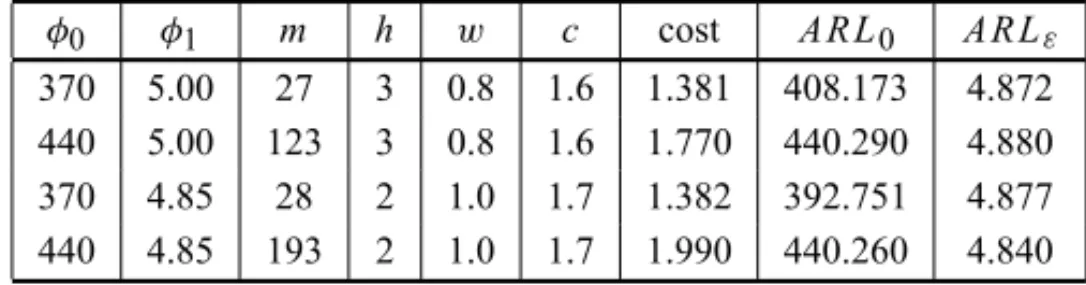
The optimum solution presented above is not influenced by the values ofφ0=370 andφ1=5, which are chosen by managers responsible for the production process because the non-restricted solution of the expression (10) [that is,m0=27;h0=3;W0=1.6,C0=3.2, $1.381] presents values of A R L0 = 408.17 and A R Lε = 4.87, which satisfy the two restrictions (φ0 = 370 andφ1=5). However, the solution may be altered depending on the values chosen forφ0and
φ1. Table 2 shows the results for some values of φ0 andφ1. An increase inφ0 (keepingφ1 constant) tends to increase the optimum interval sampling m while the values ofh, W andC
remain unaltered. An increase inφ1does not alter significantly the results; however, when both
φ0andφ1increase simultaneously, a considerable increase is observed in the sampling interval
m. The value ofmchanges from 27 to 193. As expected, the cost increases as more demanding values ofφ0andφ1are fixed.
Table 2– Optimum parameters in the functionsφ0andφ1.
φ0 φ1 m h w c cost A R L0 A R Lε
370 5.00 27 3 0.8 1.6 1.381 408.173 4.872
440 5.00 123 3 0.8 1.6 1.770 440.290 4.880
370 4.85 28 2 1.0 1.7 1.382 392.751 4.877
440 4.85 193 2 1.0 1.7 1.990 440.260 4.840
The results presented in Table 1 are very useful, but they do not help us to indicate easily which parameters have a greater impact on the cost function. Identification of such parameters is very important because the parameter values are not free of errors, and those parameters that produce more impact on the cost need more (special) attention. For that, we use a full factorial experiment with the cost as the response and the following factors: X1– the cost to inspect(ci), X2– the cost to send a non-conforming item(cn);X3– the cost to scrap an inspected item(cD),X4– the cost for adjustment(ca),X5– the process mean when the process is out-of-control(µ1)andX6 – the probability for a shift in the process mean(π ). Three levels for each factor are chosen; the value described in the beginning of this section is set as a reference level, and two other values are fixed at±15% from the reference level. Such design results in 729 possible combinations, and a multiple regression model with dummy variables will be employed. For each factor, two dummy variables are defined, as follows:
(Xj1,Xj2) =
(0,1)for 1stlevel
(1,0)for 2ndlevel (−1,−1)for 3rdlevel
the factor j isβˆj1, for the second levelβˆj2and for the third level(− ˆβj1− ˆβj2), withβˆj1and ˆ
βj2 obtained by the least squares method. The impact of factor j is proportional to the range
max(βˆj1,βˆj2,− ˆβj1,− ˆβj2)when compared with the range of the estimates of the coefficients from the other factors. Using this method, the impact of each factor is obtained and summarized in Table 3. Note that the factors X4, the cost for adjustment (ca), and X6, the probability for a shift in the process mean(π ), yield higher impacts, 31.3% and 35.1%, respectively. Thus, these factors require careful evaluation and estimation. Some descriptive statistics may help to understand these results. In Figure 4, boxplots of each factor are drawn. Observe the upward tendency of the medians of the factors pointed out as more important while the medians of the other factors are kept constant when the levels alter.
Table 3– The relative impact of the factors.
Factor Importance
cn 13.8%
cD 2.6%
µ1 16.9%
ca 31.3%
ci 0.3%
π 35.1%
5 CONCLUSIONS
In earlier papers related to this subject, the optimum corrective policy designs for Taguchi’s on-line quality monitoring procedure for variables are presented, and the sampling interval and the width of the control limits are fixed. In Ho, Medeiros & Borges (2007), the authors deter-mine the optimal sampling intervalmand the optimal control limit that minimizes the expected cost function.
In this paper, we extend the system of control by employing control zones. Three zones are stated: the green(µ0−W ≤ Xi ≤ µ0+W), yellow (µ0+W ≤ Xi < µ0+Corµ0−C <
Xi ≤ µ0−W) and red (Xi > µ0+C or Xi < µ0−C). An observed value in the green zone results in the decision that the process is in-control and the production goes on; however, one decides in favor of an adjustment of the process if the observed value belongs to the red zone; moreover, a sequential verification takes place if an observation is in the yellow zone. If a sequence ofhvalues in the yellow zone is observed, then an adjustment is decided on.
The aim is to find the values ofm,h,W andCthat minimize the average cost. According to the results presented in Section 4, the inspection control and policy presented in this paper may yield results that are at least equal to or more economical than the results obtained by Ho, Medeiros & Borges (2007).
ACKNOWLEDGMENTS
The authors would like to thank the suggestions from the two anonymous referees which have greatly contributed to the improvement of this paper. They would like to acknowledge CNPq and Fapesp for their partial financial support of this research.
REFERENCES
[1] ADAMSBM & WOODALLWH. 1989. An analysis of Taguchi’s on-line process control procedure under a random-walk model.Technometrics,31: 401–413.
[2] BORGES W, HO LL & TURNES O. 2001. An analysis of Taguchi’s on-line quality monitoring procedure for attributes with diagnosis errors.Applied Stochastic Models in Business and Industry,
17: 261–276.
[3] DASGUPTAT & MANDALA. 2008. Estimation of process parameters to determine the optimum dagnosis interval for control of defective items.Technometrics,50: 167–181.
[4] DINGJ & GONGL. 2008. The effect of testing equipment shift on optimal decisions in a repetitive testing process.European Journal of Operational Research,186: 330–350.
[5] GREENPE & SRINIVASANV. 1990. Conjoint analysis in marketing: new developments with impli-cations for research and practice.Journal of Marketing,54: 3–19.
[6] HOLL, MEDEIROSPG & BORGESW. 2007. An alternative model for on-line quality monitoring for variables.International Journal of Production Economics,107: 202–222.
[7] JIANGW & TSUIKL. 2000. An economic model for integrated APC and SPC control charts.IIE Transactions,32: 505–513.
[8] MALHOTRANK. 1999. Marketing research: an applied orientation. Prentice-Hall. Inc.
[9] NANDI SN & SREEHARIM. 1999. Some improvements in Taguchi’s economic method allowing continued quality deterioration in production process. Communications in Statistics – Theory and Methods,28(5): 1169–1181.
[10] NAKAGAWAT & OSAKIS. 1975. The Discrete Weibull Distribution.IEEE Transactions on Relia-bility,R-24 5: 300–301.
[11] NAYEBPOUR MR & WOODALL WH. 1993. An analysis of Taguchi’s on-line quality monitoring procedure for attributes.Technometrics,35: 53–60.
[12] SRIVASTAVAMS & WUY. 1995. An improved version of Taguchi’s on-line control procedure. Jour-nal of Statistical Planning and Inference,43: 133–145.
[13] SRIVASTAVAMS & WUY. 1991. A second order approximation on Taguchi’s on-line procedures. Communications in Statistics – Theory and Methods,20: 2149–2168.
[14] TAGUCHIG. 1985. Quality Engineering in Japan.Communications in Statistics – Theory and Meth-ods,14: 2785–2801.
[15] TAGUCHIG, CHOWDHURY S & WUY. 2004. Taguchi’s Quality Engineering – Handbook. John Wiley & Sons, Inc. New Jersey.
[17] TRINDADEA, HOLL & QUININOR. 2007. Monitoring process for attributes with quality deterio-ration and diagnosis errors.Applied Stochastic Models in Business and Industry,23(4): 339–358.