BOOTSTRAP CONFIDENCE INTERVALS FOR INDUSTRIAL RECURRENT EVENT DATA
Osvaldo Anacleto
1and Francisco Louzada
2*Received May 18, 2009 / Accepted June 17, 2011
ABSTRACT.Industrial recurrent event data where an event of interest can be observed more than once in a single sample unit are presented in several areas, such as engineering, manufacturing and industrial reliability. Such type of data provide information about the number of events, time to their occurrence and also their costs. Nelson (1995) presents a methodology to obtain asymptotic confidence intervals for the cost and the number of cumulative recurrent events. Although this is a standard procedure, it can not perform well in some situations, in particular when the sample size available is small. In this context, computer-intensive methods such as bootstrap can be used to construct confidence intervals. In this paper, we propose a technique based on the bootstrap method to have interval estimates for the cost and the number of cumulative events. One of the advantages of the proposed methodology is the possibility for its application in several areas and its easy computational implementation. In addition, it can be a better alternative than asymptotic-based methods to calculate confidence intervals, according to some Monte Carlo simulations. An example from the engineering area illustrates the methodology.
Keywords: industrial data, recurrent events, bootstrap, asymptotic theory, confidence intervals.
1 INTRODUCTION
In several areas, such as engineering, manufacturing and industrial reliability, we may observe recurrent event data, where the event of interest can be the repeated failures in a piece of equip-ment, systems which accumulate several repairs, or the number of bugs in a software under study, for instance. There are currently several models and methods developed for the analysis of such data, as described in Hougaard (2000). Approaches often used to model recurrent event data, which allow us to learn about an individual process, are those based on Poisson and renewal processes. (Cox & Isham, 1980; Cox & Lewis, 1966; Andersen, Borgan, Gill & Keiding, 1993; Lawless, 1987; Follmann & Goldberg, 1988; Prentice, Williams & Peterson, 1981).
*Corresponding author
For recurrent event data, it is interesting to study the number of events that occurs over the time. Adding to that, as for each event a cost can be associated, an event cost study may be also important for the analyst. From this perspective, a mean cumulative function (MCF) for the number (or cost) of events per sample unit can be defined. Nelson (1988, 1995) presented a non parametric procedure to calculate confidence intervals for this function. However, as it relies on asymptotic distributional assumptions, the quality of their results can be affected if information about the event of interest are not largely available, which results in a small sample size of units. In this context, computer-intensive methods (Davison & Hinkley, 1999; Chernik, 2008) such as bootstrap can be used to construct confidence limits for the MCF.
In this paper, we present the estimate and confidence limits proposed by Nelson, and also intro-duce a bootstrap-based technique in order to obtain confidence limits for the MCF. In Section 2, we introduce the MCF estimate proposed by Nelson (1995). Two methods to calculate con-fidence limits for the MCF are presented in Section 3, the Nelson asymptotic procedure and our proposed technique. Section 4 presents a simulation study in order to compare the two approaches discussed in Section 3 via coverage probabilities, and in Section 5 the methodol-ogy is illustrated on a valve seats replacement data set. Some concluding remarks in Section 6 finalize the paper.
2 MODEL FORMULATION AND THE MCF ESTIMATOR
Consider a population of units which are exposed to recurrent events. Despite the occurrence of censoring, an uncensored cumulative history functionYi(t)for the cost of events is associated for each population uniti. Yi(t)denotes the cumulative cost of events on uniti up to aget. The model proposed by Nelson (1995) is a population of such uncensored cumulative functions, which extend in principle to any time of interest and does not depend on the censoring of a sample.
Figure 1– Population Cumulative Cost Histories (uncensored), distribution at aget(taken from Nelson, 1995).
any aget has a finite meanC(t), which is called the population mean cumulative function per cost per unit (MCF). The MCF is represented in Figure 1 as a dark curve.
3 ESTIMATION
To estimate the population MCF, consider a sample of units which was exposed to recurrent events and their censored histories. Figure 2 shows these censored histories, where each hori-zontal line represents an unit cost history, eachx denotes an occurrence of an event, and each dashed vertical line denotes the censoring age of a sample unit.
Following Nelson (1995), note that, in the representation presented in Figure 2, the units are shown in an ascending order and numbered backward according to their censoring ages. Also, these censoring ages divide the observed age range intoNintervals, as well as these intervals are also numbered backward. Denote the total incremental event cost accumulated over all events in intervali on unitnbyYi n wherei,n =1,2, . . . ,N. Based on this representation, the estimate for the mean cost cumulative function at a given agetin the intervalI is,
C∗(t) = 1
N
YN N +YN,N−1+YN,N−2+ · · · +YN I + · · · +YN1
+ 1
N−1
YN−1,N−1+YN−1,N−2+ · · · +YN−1,I+ · · · +YN−1,1
+ 1
N−2
YN−2,N−2+ · · · +YN−2,I+ · · · +YN−2,1
..
. . .. ... ...
+ 1
I+1
YI+1,I+1+YI+1,I+ · · · +YI+1,1
+ 1
I
YI,I+ · · · +YI,1.
(1)
Note that the first row in (1) denotes the total incremental cost of N units in the interval N divided byN, the second row denotes the total incremental cost of N −1 units in the interval N −1 divided by N −1 and so on. The sum in the last row is the total incremental cost up to aget of all I units which are exposed in interval I. It implies that each row represents the average incremental cost per unit for each interval from N up to I. Since the MCF estimate depends on the intervals which have considered for the representation in Figure 2, this estimate and also the confidence limits are conditional on the given censoring ages. Also, it is assumed that the set of units considered for the estimate are a random sample from some population, and the event histories for each unit are statistically independent of their censoring ages. To avoid consideration of ties, it is assumed the the sample ages of recurrences are known exactly and are distinct points on a continous time scale. Note that the estimate for the mean number cumulative function is the same except that 1 is used as the cost for each event.
→
←
→
←
→
←
→
←
→
←
→
←
→
←
→
←
→
←
→
←
→
←
→
←
→
←
→
←
→
←
→
←
→
←
→
←
→
←
→
←
→
←
→
←
→
←
→
←
→
total incremental costs in (1) and the covariances V(Yi n,Yj,n), which reflects the population autocorrelation between incremental cost in intervalsiand j. Then the variance of (1) is,
V[C∗(t)] = 1
N2
V(YN N)+V(YN,N−1)+V(YN,N−2)+ · · · +V(YN I)+ · · · +V(YN1)
+ 1
(N−1)2
V(YN−1,N−1)+V(YN−1,N−2)+ · · · +V(YN−1,I)+ · · · +V(YN−1,1)
+ 1
(N−2)2
V(YN−2,N−2)+ · · · +V(YN−2,I)+ · · · +V(YN−2,1)
. .
. . .. ... ...
+ 1
(I+1)2
V(YI+1,I+1)+V(YI+1,I)+ · · · +V(YI+1,1)
+ 1
I2
V(YI,I)+ · · · +V(YI,1)
− − − − − − − − − − − − − − − − − − − − − − − − − − − − − − − − − −
V[C∗(t)] = + 2
N(N−1)
N−1
X
n=1
V(YN n,YN−1,n)
+ 2
N(N−2)
N−2
X
n=1
V(YN n,YN−2,n)
+ 2
N(N−3)
N−3
X
n=1
V(YN n,YN−3,n)
. .
. ...
+ 2
N(I+1)
I+1
X
n=1
V(YN n,YI+1,n)
+ 2
N I I
X
n=1
V(YN n,YI,n)
− − − − − − − − − − − − − − − − − − − −
+ 2
(N−1)(N−2)
N−2
X
n=1
V(YN−1,n,YN−2,n)
+ 2
(N−1)(N−3)
N−3
X
n=1
V(YN−1,n,YN−3,n)
+ 2
(N−1)(N−4)
N−4
X
n=1
V(YN−1,n,YN−4,n)
. .
. ...
+ 2
(N−1)(I +1)
I+1
X
n=1
V(YN−1,n,YI+1,n)
+ 2
(N−1)I I
X
n=1
V(YN−1,n,YI,n)
− − − − − − − − − − − − − − − − − − − −− . . . ... − − − − − − − − − − − − − − − − − − − −− 2
(I+1)I I
X
n=1
V(YI+1,n,YI,n).
(2)
The first block of terms consists of the individual variances of each of theYi nin (1), the second block consists of the covariances between incremental costs in intervali =N and those of each in subsequent intervalsi =N −1, i =N−2, . . . ,i = I. The third block of terms consists of the covariances between incremental costs in intervali =N−1 and those of each in subsequent intervalsi = N −2, i = N −3, . . . ,i = I and so on until the last block, which consists of the covariances between incremental costs in intervali = I+1 and those in the intervali =I up to aget.
Since the variances appearing in the first row of the first block in (2) areN independent observa-tions from the same incremental cost distribution for the intervalN, we have
V(YN N)=V(YN,N−1)=. . .=(YN1)=V(YN n).
Hence, the sum of the first row of the first block in (2) is N V(YN n). By this reasoning, the N −1 variances in the second row of the first block have a common value V(YN−1,n)and a sum of(N −1)V(YN−1,n)and so on. Similarly, the covariance terms can be combined, since the covariance terms in a sum in a single row of (2) are all equal. For instance, the first row of the second block has N−1 covariances with a common value V(YN n,YN−1,n)and a sum of
(N−1)V(YN n,YN−1,n). Hence, the variance of theC∗(t)can be simplified as
V[C∗(t)] = 1
NV(YN n)+ 1
N−1V(YN−1,n)+ 1
N−2V(YN−2,n)+ · · · + 1 IV(YI n)
+ 2
N[V(YN n,YN−1,n)+V(YN n,YN−2,n)+ · · · +V(YN n,YI,n)]
+ 2
N−1[V(YN−1n,YN−2,n)+ · · · +V(YN−1n,YI,n)] + · · ·
· · · + 2
I+1[V(YI+1n,YI,n)].
For the estimation of the terms in (3), consider thei sample incremental costsYii,Yii−1,...,Yi1 observed in interval i. These observed costs are a random sample from the incremental cost distribution of the intervali. Thus, their sample variance,
V∗(YI n)= +1
I i
X
n=1
(Yi n−Y i)2 (4)
is an unbiased estimate of the population variance V(Yi n). Also, the population covariance V(Yi n,Yj n)is estimated by the sample covariance,
V∗(YI N,YI J) = + 1 J−1
J
X
n=1
(Yi n−Y i)(Yj n−Yj). (5)
J<I.
The inclusion of (4) and (5) into (3) provides an unbiased estimate for the true varianceV[C∗(t)]
(Nelson, 1995).
4 CONFIDENCE INTERVALS FOR MCF
In this Section, the usual procedure to calculate confidence limits for the Mean Cumulative Function are presented, as well as an alternative based on bootstrap techniques.
4.1 Confidence Intervals Based on Asymptotic Theory
Suppose thatNcumulative history functions for cost represented in Figure 2 are a simple random sample from a infinite population. At a given time t, the estimator of the Mean Cumulative Function estimator is given by (3). Since this estimator is the sample mean considering censored histories, by the central-limit theorem (Lehmann, 1999),C∗(t)has a normal distribution with MeanC(t)(the mean cumulative function at the timet) and varianceV∗[C∗(t)](Nelson, 1995). Hence, the two sided normal approximate(100−α)% confidence interval forC(t)is given by,
C∗(t)±Kα∗ {V∗[C∗(t)]}1/2 (6)
whereV∗[C∗(t)]is theV[C∗(t)]estimator andK
αis theα/2 standard normal percentile.
This procedure are based on a sample of units, in which the asymptotic based confidence intervals presented here can not perform well if the size sample is small. In this context, computer-intensive methods such as bootstrap can be used to construct confidence intervals for the Mean Cumulative Function.
4.2 Confidence Intervals Based on the Bootstrap
basic idea is to consider the observed data as a population, and then samples from this population are obtained based on a sampling scheme with replacement from the original sample. If this procedure is repeated several times, different values of the quantities of interest can be obtained, thus providing an empirical distribution of this quantity. Based on this idea, it is possible to construct the percentile confidence intervals (Efron & Tibshirani, 1993; Davison & Hinkley, 1999; Chernik, 2008; Souza, Souza & Staub, 2009) for the MCF, resampling the original set of units exposed to recurrent events and calculating the mean cumulative function estimate for each sample available.
Along these lines, an algorithm to obtain the 100(1−α)% percentile bootstrap confidence in-tervals for the MCF is given by the following steps:
Step 1: From the original dataset, obtainBresamples of units based on a sampling with replace-ment scheme;
Step 2: To each of the Bresamples, calculate the Mean Cumulative Function estimate;
Step 3: Based on the estimates obtained from the resamples of the original dataset, calculate the α
2 and 1− α 2
percentiles from the empirical distributions for each recurrent time for the units from the original dataset, provided for theBsets of estimatives calculated from the B resamples.
A program to calculate the bootstrap confidence intervals for the MCF is available from the authors. An implementation of the variance estimate of (3) as well as asymptotic confidence limits are provided by the SAS software.
5 A SIMULATION STUDY
In order to assess the efficiency and have a comparison of the confidence intervals provided by the asymptotic theory and the bootstrap, as well as verifying the sample size influence in these methods, a simulation study was performed to check the coverage probability and the mean range of the confidence intervals developed here.
The study considered the sample sizes of 10, 30 and 100. For each sample size, four scenarios based on the parameter settings for the data generation were considered: the number of events in each sample unit was generated from a Poisson distribution with means 2 and 5, and the recurrence times were generated from an Weibull distribution with scale parameter 1000 and shape parameter equal to 1 and 3, assuming the biggest time generated for each unit as a censored event. We considered then four different scenarios: Scenario 1 (Poisson distribution with mean equals to 2 and Weibull distribution with shape equals 1), Scenario 2 (Poisson distribution with mean equals to 2 and Weibull distribution with shape equals 3), Scenario 1 (Poisson distribution with mean equals to 5 and Weibull distribution with shape equals 1) and Scenario 1 (Poisson distribution with mean equals to 5 and Weibull distribution with shape equals 3). It was not considered the presence of ties. We studied the behavior of the 90% confidence limits for the mean number cumulative function, which is a MCF particular case.
399. According to Hall (1986) this number of replications is enough to obtain a critical level of 0.05 from the 0.95 percentile of the empirical distribution of the test statistics. To set up the Monte Carlo simulation, this procedure was repeated 399 times. The MCF estimate was calculated for each of the samples. In order to calculate the coverage probability, it was necessary to set percentiles, since the recurrence times from the 399 samples and the original sample were generated from a probability distribution, thus varying from sample to sample. The percentiles 10, 25, 50, 75 and 90. where chosen. With this, for each considered percentile it was verified whether the confidence intervals of the 399 samples covered the MCF estimate obtained in the original sample. If not, it was also verified if the related percentile MCF estimate lied above the upper limit or below the lower limit.
The results for all scenarios considered are presented are presented in Table 1. It contains, for each verified percentile, the time related to the percentile in the original sample, and, for the two methods considered, the coverage probability, the average range of the interval and the standard deviation of the interval range in the 399 samples apart from the original sample. The relative difference of these quantities between the methods is also presented, always considering the quantity provided by the asymptotic method in the denominator.
For sample sizes bigger than 30, in all the scenarios, it was verified that the bootstrap method and the asymptotic method provides similar coverage probabilities. Besides, the results indicate that the coverage probabilities are underestimated in the smallest percentiles and overestimated in the biggest quantiles, and it tends to decrease as the sample size increases as well as the average confidence intervals and its standard deviations do. However, for the sample size 10, the bootstrap method provides smaller confidence intervals average ranges as well as smaller standard deviations of these ranges. It indicates that, since the asymptotic methods requires a sufficiently large sample for developing inferences, the bootstrap method can be used as an alternative approach to provide confidence limits for the mean cumulative function in presence of small samples.
6 THE VALVE SEATS REPLACEMENT DATA
The presented methodology was applied to a real dataset provided by Nelson (1995). The data is the valve seats replacement over the time in 41 engines in a fleet. Is this case, the recurrent event is the valve seats replacements in each of the engines. The interest relies on verifying if the replacement rate increases with engine age (in days).
100 200 300 400 500 600 0 .0 0 .5 1 .0 1 .5 2 .0
time (in days)
M C F e st im a te a n c co n fi d e n ce l im it
s MCF estimate
95% asymptotic confidence interval 95% bootstrap confidence interval
Figure 3– 95% Asymptotic and bootstrap Confidence Intervals for the MCF.
one. Even though these results are not conclusive, they provide an indication of the advantage of the pratical use of the boostrap confidence interval procedure over the asymptotic method.
7 CONCLUDING REMARKS
In this work, we presented the estimate and confidence intervals based in the asymptotic theory proposed by Nelson (1995) for the Mean Cumulative Function, using non parametric methodol-ogy for recurrent events data. Also, it was presented an implementation of the bootstrap tech-nique for the construction of confidence limits for the MCF. These two procedures were applied in a real dataset. One of the advantages of the proposed methodology presented here is the possibility for its application in several areas, its easy computational implementation.
Our simulation results suggest that the confidence intervals based on the two procedures are similar to moderate and large sample sizes. However, for small sample sizes, the bootstrap method provides smaller confidence intervals ranges as well as smaller standard deviations of these ranges. Hence, the bootstrap method can be used as an alternative approach to provide confidence intervals for the Mean Cumulative Function, in particular when there are restrictions regarding the availability of information about the event under study.
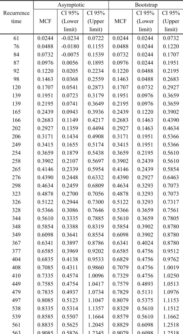
Table 2– 95% asymptotic and bootstrap Confidence Intervals for the MCF.
Asymptotic Bootstrap
Recurrence CI 95% CI 95% CI 95% CI 95%
time MCF (Lower (Upper MCF (Lower (Upper
limit) limit) limit) limit)
61 0.0244 -0.0234 0.0722 0.0244 0.0244 0.0732
76 0.0488 -0.0180 0.1155 0.0488 0.0244 0.1220
84 0.0732 -0.0075 0.1539 0.0732 0.0244 0.1707
87 0.0976 0.0056 0.1895 0.0976 0.0244 0.1951
92 0.1220 0.0205 0.2234 0.1220 0.0488 0.2195
98 0.1463 0.0368 0.2559 0.1463 0.0488 0.2683
120 0.1707 0.0541 0.2873 0.1707 0.0732 0.2927
139 0.1951 0.0723 0.3179 0.1951 0.0976 0.3659
139 0.2195 0.0741 0.3649 0.2195 0.0976 0.3659
165 0.2439 0.0943 0.3936 0.2439 0.1220 0.3902
166 0.2683 0.1149 0.4217 0.2683 0.1463 0.4390
202 0.2927 0.1359 0.4494 0.2927 0.1463 0.4634
206 0.3171 0.1434 0.4908 0.3171 0.1951 0.5366
249 0.3415 0.1655 0.5174 0.3415 0.1951 0.5366
254 0.3659 0.1879 0.5438 0.3659 0.2195 0.5610
258 0.3902 0.2107 0.5697 0.3902 0.2439 0.5610
265 0.4146 0.2339 0.5954 0.4146 0.2439 0.5854
276 0.4390 0.2448 0.6332 0.4390 0.2927 0.6463
298 0.4634 0.2459 0.6809 0.4634 0.3293 0.7073
323 0.4878 0.2700 0.7056 0.4878 0.3293 0.7073
326 0.5122 0.2944 0.7300 0.5122 0.3293 0.7317
328 0.5366 0.3086 0.7646 0.5366 0.3659 0.7561
344 0.5610 0.3335 0.7885 0.5610 0.3659 0.7805
348 0.5854 0.3388 0.8319 0.5854 0.3902 0.8780
349 0.6098 0.3641 0.8554 0.6098 0.3902 0.8780
367 0.6341 0.3897 0.8786 0.6341 0.4024 0.8780
377 0.6585 0.3969 0.9202 0.6585 0.4756 0.9512
404 0.6835 0.4138 0.9533 0.6829 0.4756 0.9762
408 0.7085 0.4311 0.9860 0.7079 0.4756 1.0019
410 0.7335 0.4574 1.0096 0.7329 0.4756 1.0250
449 0.7585 0.4754 1.0417 0.7579 0.4893 1.0513
479 0.7835 0.4937 1.0734 0.7829 0.5131 1.0976
497 0.8085 0.5123 1.1047 0.8079 0.5375 1.1153
538 0.8335 0.5314 1.1357 0.8329 0.5610 1.1512
539 0.8585 0.5507 1.1664 0.8579 0.5610 1.1662
561 0.8835 0.5625 1.2045 0.8829 0.6098 1.2518
Table 2(continuation) – 95% asymptotic and bootstrap Confidence Intervals for the MCF.
Asymptotic Bootstrap
Recurrence CI 95% CI 95% CI 95% CI 95%
time MCF (Lower (Upper MCF (Lower (Upper
limit) limit) limit) limit)
570 0.9335 0.5955 1.2716 0.9329 0.6491 1.2768
573 0.9585 0.6232 1.2938 0.9579 0.6491 1.2768
581 0.9849 0.6451 1.3246 0.9829 0.6829 1.3369
586 1.0143 0.6692 1.3593 1.0092 0.7082 1.3369
604 1.0597 0.6920 1.4275 1.0387 0.7340 1.4202
621 1.1185 0.7048 1.5323 1.0841 0.8170 1.5715
635 1.1810 0.7685 1.5936 1.1429 0.8170 1.5715
640 1.2435 0.7911 1.6959 1.2054 0.8840 1.6409
646 1.3205 0.8635 1.7774 1.2679 0.8840 1.7201
653 1.4316 0.9232 1.9399 1.3449 0.9702 2.1313
653 1.5427 0.9079 2.1774 1.4560 0.9702 2.1313
such as the normal, percentile t and the pivotal method (Davison & Hinkley, 1999; Chernik, 2008), can also be considered in the context of obtaining confidence intervals for the MCF.
ACKNOWLEDGMENTS
We would like to thank the referees for their very useful comments which substantially improved the paper. The research was partially supported by the Brazilian Organizations CAPES and CNPQ.
REFERENCES
[1] ANDERSENPK, BORGANO, GILLRD & KEIDING. 1993.Statistical Models Based on Counting Processes. New York: Springer.
[2] COXDR & LEWISPAW. 1966.The Statistical Analysis of Series of Events. London: Methuen.
[3] COXDR & ISHAMV. 1980.Point Processes. London: Chapman and Hall.
[4] CHERNICKMR. 2008.Bootstrap Methods: A Guide For Practitioners and Researches. New York: Wiley.
[5] DAVISONAC & HINKLEYDV. 1997.Bootstrap Methods and Their Application. Cambridge Uni-versity Press.
[6] EFRON B. 1979. Bootstrap methods: Another look at the jackknife. The Annals of Statistics, 7: 1–26.
[7] EFRONB & TIBSHIRANIRJ. 1993.An introduction to the bootstrap. New York: Chapman & Hall.
[9] HALLP. 1986. On the number of bootstrap simulations required to construct a confidence interval.
The Annals of Statistics,14: 125–129.
[10] HOUGAARDP. 2000.Analysis of Multivariate Survival Data. New York: Springer-Verlag.
[11] LAWLESSJF. 1987. Regression methods for Poisson process model.Journal of the American Statis-tical Association,82: 808–815.
[12] LEHMANNEL. 1999.Elements of Large-sample Theory.New York: Springer-Verlag.
[13] MORETTIAR & MENDESBVM. 2003. Sobre a precis˜ao das estimativas de m´axima verossimilhanc¸a nas distribuic¸˜oes bivariadas de valores extremos.Pesquisa Operacional [online],23(2): 301–324.
[14] NELSONW. 1988. Graphical Analysis of System Repair Data.Journal of Quality Technology,20: 24–35.
[15] NELSONW. 1995. Confidence Limits for Recurrence Data-Applied to Cost or Number of Product Repair.Technometrics,37: 147–157.
[16] PRENTICERL, WILLIAMSBJ & PETERSONAV. 1981. On the regression analysis of multivariate failure time data.Biometrika,68: 373–379.