RBRH, Porto Alegre, v. 22, e32, 2017
Scientiic/Technical Article
http://dx.doi.org/10.1590/2318-0331.011716071
Coupling the atmospheric model RAMS 6.0/ECHAM 4.1 to hydrologic
model SMA/HMS for operating a reservoir in Brazil’s semiarid
Acoplamento do modelo atmosférico RAMS 6.0/ECHAM 4.1 ao modelo hidrológico SMA/HMS para operação do Reservatório Orós no semiárido brasileiro
Samuellson Lopes Cabral1, José Nilson Bezerra Campos2 and Cleiton da Silva Silveira3
1Centro Nacional de Monitoramento e Alertas de Desastres Naturais, São José dos Campos, SP, Brasil 2Universidade Federal do Ceará, Fortaleza, CE, Brasil
3Universidade da Integração Internacional da Lusofonia Afro-Brasileira, Redenção, CE, Brasil
E-mails: [email protected] (SLC), [email protected] (JNBC), [email protected] (CSS)
Received: May 27, 2016 - Revised: October 13, 2016 - Accepted: November 28, 2016
ABSTRACT
The planning and the eficiency of water resources are subject to the uncertainties of the input data of climate and hydrological models. Prediction of water inlow to reservoirs that would help decision making for the various water uses, contain uncertainties fundamentally the initial conditions assumed in the modeled processes. This paper evaluates the coupling of a regional atmospheric model with a hydrological model to make streamlow forecast for seasonal operation of Orós reservoir, Ceará State, Brazil. RAMS model, version 6.0, was forced by the ECHAM 4.5 atmospheric general circulation model over Alto Jaguaribe basin to obtain the rainfall data. To remove biases in the simulated precipitation ields was applied the probability density function (PDF) correction on them. Then the corrected precipitation data were inserted in the hydrologic Soil Moisture Account (SMA) model from the Hydrologic Modeling System (HEC-HMS). For SMA calibration, it was used the Nash-Sutcliffe objective function. Finally, decisions to water release from the Orós were evaluated using the Heidke Skill Score (HSS). The SMA model showed a satisfactory performance with Nash-Sutcliffe values of 0.92 (0.87) in the calibration (validation) phase, indicating that it is a rainfall runoff model alternative. For decisions in releasing water from the Orós reservoir, using climate predictions, obtained HSS = 0.43. The results show that the simulated rainfall coupled with a hydrological model is able to represent the hydrological operation of Brazilian semiarid reservoir.
Keywords: Soil Moisture Account; Flow forecast; Reservoir management.
RESUMO
O planejamento e a eiciência dos recursos hídricos estão sujeitos às incertezas decorrentes dos dados de entrada de modelos climáticos e hidrológicos. Previsão de vazões aluentes a reservatórios que auxiliariam as tomadas de decisões para os diversos usos da agua, contem incertezas fundamentalmente das condições iniciais assumidas nos processos modelados. Nesse contexto o artigo avalia a eiciência do acoplamento do modelo atmosférico ao modelo hidrológico, com vistas a utilizar a previsão climática na operação sazonal do reservatório Orós, no estado do Ceará. O modelo atmosférico regional RAMS 6.0 foi forçado pelo modelo atmosférico global ECHAM 4.5, na bacia hidrográica do Alto Jaguaribe para obtenção dos dados de precipitação. Para retirar vieses nas precipitações, foi aplicada a correção função densidade de probabilidade (PDF) nos dados simulados. Em seguida, os dados de precipitações foram inseridos no modelo hidrológico Soil Moisture Account (SMA) do Hydrologic Modeling System (HEC-HMS). Para a calibração do SMA, foi usada a função objetivo Nash-Sutcliffe. Por im, foram avaliadas as decisões de liberação do Orós, utilizando o Heidke Skill Score (HSS). O SMA apresentou acurácia, com valores de Nash-Sutcliffe de 0,92 na fase de calibração, e 0,87 na fase de validação, mostrando ser uma alternativa de modelo precipitação delúvio. Para as decisões na liberação de águas do reservatório, utilizando-se as previsões climáticas, obteve-se HSS =0,43. Os resultados mostram que as previsões de precipitação acopladas a um modelo hidrológico se constituem em promissora ferramenta para a operação hidrológica de reservatórios do Semiárido brasileiro.
INTRODUCTION
Semiarid regions, such as the Northeast of Brazil (NEB), are particularly vulnerable to climate luctuations and their impact on water supply shortage. Forecast models of rivers discharges for a few months or a year’s horizon time are an interesting research topic from the viewpoint of achieving more eficient operation of water supplies and water allocation among competing uses and users (SOUZA FILHO; LALL, 2004).
Issues such as the prevention and lood control, reservoir operation, and the planning of water use are directly associated with the prediction of rivers discharges, which present uncertainties arising essentially from the modeling process and the assumptions of the model initial conditions (GEORGAKAKOS et al., 2005; DOBLAS-REYES et al., 2005).
Most of the water supply for the Ceará cities relies on these network reservoirs. However, currently, there are few possibilities for building new reservoirs to increase water availability. In this context, it has become increasingly important to seek better water management practices, including better reservoir inlow forecasts and improved reservoir operations.
Discharges forecast are into two categories: statistics or deterministic. The irst uses historical records of climatic variables and low rates, which allow future lows to be represented based on the probable behavior of the observed series. The second seeks to represent the processes of the hydrological cycle through a combination of atmospheric and hydrological modeling, thus providing a physical representation of hydro climatic processes of a given river basin (SOUZA FILHO; LALL, 2003).
Dynamic and statistical methods are used to develop estimates of long time horizon discharges, which can be used for allocation and operation of water resources to competing demands. Some research has been conducted successfully in semi-arid regions of NEB and Amazon with climate information to predict low rates, demonstrating that the seasonal forecast has signiicant predictive accuracy when weather information is provided (MOURA; SHUKLA, 1981; SOUZA FILHO; LALL, 2003; UVO; BERNDTSSON, 2000; BLOCK et al., 2009; BLOCK; RAJAGOPALAN, 2009).
Sun et al. (2005) developed a dynamic downscaling forecast system for NEB and have generated predictions of seasonal rainfall since December 2001. The ECHAM 4.5 and the Regional Spectral Model (Regional Spectral Model-RSM/NCEP) constitute the core of this system. Forecasts of the sea surface temperature (SST) are initially produced as a condition of contour, forcing the lower bound for the nested system ECHAM 4.5-NCEP RSM.
Some researchers (PIELKE et al., 1992; COTTON et al., 2003) conducted experiments with the Regional Atmospheric Modeling System – model RAMS 6.0 for NEB, to improve the predictions of their system, and increase the spatial resolution of the information generated.
The forecast skill depends on the ability of representation of natural processes associated with the weather system, as well as the characteristics of the model or the set of models (spatial resolution, quality of the representation of physical processes, quality of initial conditions assumed, etc.). In terms of the reliability, improved understanding of the sensitivity and limitations of the forecast system is crucial to ensuring that the system can deine
policies of the planning and management of water resources (REIS JÚNIOR, 2009).
In NEB, seasonal rainfall forecasts are made, initially, on a daily time scale. In this range, the models feature low predictability (skill), and therefore, precipitation is grouped in larger intervals of months or years. For hydrological forecast, the practice is to use a monthly and/or annual time scale.
To test a new model of coupled atmospheric models, i.e., hydrological models applied to reservoir operation, the model x lood Soil Moisture Account-SMA is used. SMA is a tool of the program HEC-HMS. It has been used successfully by several researchers worldwide (BENNETT; PETERS, 2000; GARCÍA et al., 2008; CHU; STEINMAN, 2009; BASHAR, 2012; GOLIAN et al., 2012; KOCH; BENE, 2013; GYAWALI; WATKINS, 2013). However, for the Brazilian semi-arid region, there is limited research on the application of SMA in hydrological forecasts.
The main objective of this article is to evaluate the performance of coupling the seasonal rainfall forecasts of RAMS 6.0 to the hydrological model SMA in a watershed semi-arid region of the NEB, for the seasonal operation of a reservoir. The model is applied to the high Jaguaribe valley with the Jaguaribe River, an area that has great social and environmental and economic inluence. The methodology developed here can be an important tool to evaluate the risks associated with the variability of seasonal climate and the construction of seasonal adaptation strategies to manage hydroclimatic risk management.
DATA AND DESCRIPTION OF APLICATION SITE
High Jaguaribe River Basin
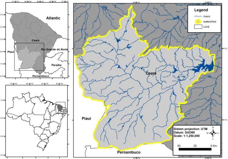
Located in the southwest of the State of Ceará, the High Jaguaribe Valley (Figure 1) has an area of 24.538 km2. The river
Jaguaribe, which is 633 km long in total, traverses approximately 325 km up to the reservoir Orós. The average annual rainfall in the area ranges from 500 to 700 mm, with high irregularity in time and space. The main weather system in the area is the intertropical convergence zone (ITCZ), with greater intensity in the months of March and April. In the so-called pre-season, from December to February, the basin receives rainfall from the inluence of cold fronts, which are located in the central northern sector of the northeast, and nearby cyclonic vortices of high levels (VCANs). From May to June, precipitation falls under the Eastern wave system.
The Jaguaribe River regime in Iguatu has an annual average low of 24.45 m3/s and standard deviation of 37.8 m3/s. In the second semester, under natural conditions, the river remains completely dry. This peculiar concentration of lows and rainfall can be seen in the histogram and the mean annual hydrograph (Figure 2).
Rainfall data
The data cover the period from 1979 to 2009. The average precipitation in the basin was estimated by the Thiessen polygon method (THIESSEN, 1911).
Streamlow data
The Jaguaribe River discharge data were obtained from the National Agency of Water (ANA). The data cover a period from 1912 to 2009 with some missing data. ECHAM 4.5 and RAMS
precipitation data were provided by FUNCEME. The Iguatu luviometric station provided the most reliable streamlow data in the study area.
Dynamic model of precipitation
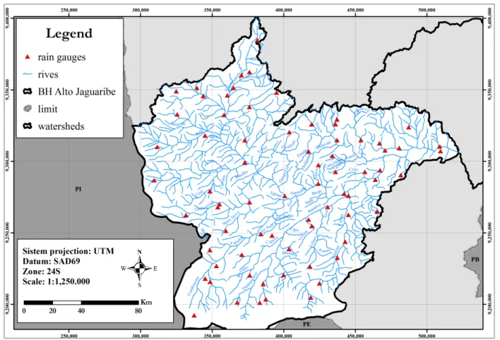
Monthly precipitations in the irst semester were simulated by the model RAMS 6.0 precipitation encompassing the period from 1979 to 2009. It was applied over a 30 × 30 km2 grid, from which the average daily precipitation over the basin was obtained. Figure 4 shows the spatial distribution of the posts used and only the RAMS 6.0 grid points.
The RAMS 6.0 was initialized with the ECHAM 4.5 data. The simulation was made with Newtonian relaxation scheme (nudging), proposed by Davies (1976), by adding a term to the basic equations, which causes the value of each variable in the various grid points to retain large-scale information. The assimilation was made by side borders, on the top and in the center of the model domain (side, top, and center nudging). For the statistical calculations, these lateral points were disregarded, considering that the same have noises caused by the Newtonian relaxation scheme of the regional model.
The model RAMS 6.0 was conigured with a polar stereographic grid covering the whole NEB and a portion of the
Figure 1. High Jaguaribe River Basin.
Figure 2. Rainfall and streamlow seasonality in the High Jaguaribe
Figure 4. Spatial distribution of RAMS 6.0 grid points in High Jaguaribe Valley.
tropical area surrounding the Atlantic Ocean, with 100 points in both directions, a horizontal spacing of 30 km, and the center located at 8° S, 40° W. The vertical grid, with 38 levels, had variable spacing from 50 m near the surface of the soil to 1100 m at the top of the troposphere. The parameterizations adopted include Mellor and Yamada (1974) for turbulence, Walko et al. (1995) for cloud microphysics, Chen and Cotton (1983) for radiation, and Kuo modiied (KUO, 1974) for convection.
The TSM monthly average observed in the Paciic, Atlantic, and Indian oceans, in the months from January to December (1979-2009) served as contour variables to the surface in the simulations of the ECHAM 4.5 and 6.0 RAMS. ECHAM 4.5 and RAMS 6.0 generated the output of 10 sets of daily rainfall.
Various researchers (TOTH; KALNAY, 1993; MOLTENI et al., 1996) agree that the best estimate of climate variables, especially for medium-term simulation, is the average of the sets (ensemble), mainly in a deterministic approach. In this study, an average of 10 sets of daily rainfall was adopted for precipitation forecast. The daily values were then grouped into monthly igures that show a higher predictability (CABRAL et al., 2016).
The correction of rainfall, to remove bias, was made with the transformation of empirical probability distribution curve of monthly precipitation. For each month of the year and for each climate model grid point, two empirical probability distribution curves are developed: the observed data and the predicted values of monthly precipitation.
Hydrologic model
The hydrological model HEC-HMS is conigured using the soil moisture accounting method (SMA) for the water budget in the basin (BENNETT; PETERS, 2000), the SCS unit hydrograph to obtain the surface hydrograph, the linear reservoir to route the groundwater (RAUDKIVI, 1979), and the Muskingum-Cunge method for propagation on the rivers (CUNGE, 1969). The SMA requires knowledge of 14 parameters. The parameters were estimated initially based on physiographic characteristics of the basin, as proposed by Bennett and Peters (2000). The SMA model uses hypothetic reservoirs to represent the storage and the movement of water in the surface layer of soil, saturated zone in the upper layer, and in the bottom layer of the saturated zone.
Calibration and validation of SMA
The observed series of precipitation and discharges were used for calibration of the SMA parameters, and for estimation of the skill of the coupled model. The period chosen for calibration was 1979-1995 and for validation was 1996–2009. These periods present similarities in terms of the extreme lows. The calibration was performed initially in an automatic way, according to the HEC-HMS version of the multiobjective optimization algorithm. For the parametric calibration of the SMA, the Nash-Sutcliffe coeficient (NASH; SUTCLIFFE, 1970) was applied.
Decisions on reservoir operation
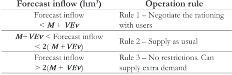
Decisions on the Orós reservoir operation are evaluated under the assumption that the volume of the reservoir at the beginning of the year (S0) is insuficient to meet the demand. This represents a critical situation, in which the decision is made to meet the demands using all available water or to promote rationing. Release rules are evaluated as functions of the low regulated by the reservoir (M), volume of average annual losses by evaporation (VEv), and the volume of water provided for the wet season (VAp), as determined by the climatic and hydrological forecast. Table 1 summarizes the scenarios of operational decisions for the management of the Orós reservoir.
The reservoir yield M and evaporative losses are estimated by the method of Regulation Triangular Diagram (RTD). The method provides the solution of the dimensionless equation of water balance using the Monte Carlo simulation technique. The solution uses three parameters: the dimensionless factor of evaporation (fE), the dimensionless factor of capacity (fK), and the coeficient of variation and annual inlows (CV) (CAMPOS, 2010).
The eficiency of the decisions for deining the rules of operation of the Orós reservoir was evaluated with the HSS metric (HEIDKE, 1926), as follows:
( ) ( ) ( ) ( ) ( ) 2 1 1 2 1 1 1 1 1 − − ∑ ∑ ∑ k k
i i i i
i= i=
k
i i i=
N F O N F N O
N N
HSS =
N F N O
N
(1)
where N (Fi, Oi) denotes the number of predictions in category i that includes observations in category i; N (Fi) indicates the total number of predictions in category i; N (Oi) represents the total number of observations in category I; N is the total number of observations; and k is the number of classes.
Cascade model: summary
The ECHAM 4.5, forced by the TSM global observed during 1979-2009, generated the irst series of ten sets of precipitations in low spatial resolution. The outputs of the ECHAM 4.5 forced the RAMS 6.0 to obtain ten new sets of rainfall in the area of the basin, with higher spatial resolution. To remove biases, the PDF correction technique was applied to the series of monthly precipitation from RAMS 6.0. This technique consists of calculating the monthly probability density function (pdf), and applying the ix, as shown in Figure 5, according to Block et al. (2009). This paper used the cascade model, which is shown in Figure 6.
Table 1. Rules for release water based on discharges forecast. Forecast inlow (hm3) Operation rule
Forecast inlow
< M + VEv
Rule 1 – Negotiate the rationing with users
M+VEv < Forecast inlow
< 2( M +VEv) Rule 2 – Supply as usual
Forecast inlow
> 2(M + VEv)
Rule 3 – No restrictions. Can
supply extra demand
The observed and simulated rainfall series were applied to SMA. Two series were obtained: the inlow volumes simulated with observed average rainfall (VPMED), and the series of inlows volumes simulated with forecast rainfall ECHAM 4.5/6.0 RAMS (VRAMS). The modeling eficiency was evaluated with the following metrics: mean square errors deviation, NS, and HSS. The VRAMS series was used to deine the application of inlow forecast release decisions from the Orós reservoir. The evaluation of the eficiency of the release decisions was made with the HSS metric. A comparison was made between the decisions with the observed lows and the lows of the climate-hydrological forecast.
RESULTS AND DISCUSSIONS
SMA calibration and validation
Table 2 shows the SMA parameters values. The following parameters were more sensitive on the river discharges: maximum soil iniltration (2.5 mm/h), storage in the soil (45 mm), storage in tension zone (30 mm), impermeable area (15%), soil percolation (1.5 mm/h) and storage in the surface layer (2.0 mm). The values of the parameters calibrated with the observed data for the January–June period of 1979 to 1995 feature NS values equal to 0.92. With the calibrated parameters, the model was validated with data from the January–June period of 1996 to 2009. In the validation step, the NS obtained was equal to 0.87.
The NS is widely used in hydrological studies, because it is highly inluenced by extreme values, and is therefore very sensitive to loods events. This fact explains the better performance of the model for the validation period, since the lowest occurrence of extreme peaks of low when compared to the calibration period.
For the precipitation models x lood, several studies report acceptable NS values ranging from 0.36 to 0.75. With the SMA of the HEC-HMS in six basins in Northern Spain, the NS values obtained were 0.52-0.79 in the calibration phase and 0.36-0.75 in the validation phase (COLLISCHONN, 2001; GARCÍA et al., 2008). Therefore, compared with other applications of SMA, the NS values found in this paper can be considered to be good.
Figure 6. Schematic representation of cascade model.
Table 2. Calibrated parameters for SMA model applied to High Jaguaribe Valley at Orós reservoir.
Parameters Initial value
Soil (%) 1
Groundwater 1 (%) 0
Groundwater 2 (%) 0
Max Iniltration (mm/h) 2.5
Impervious (%) 15
Soil Storage (mm) 45
Tension Storage (mm) 30
Soil Percolation (mm/h) 1.5
GW 1 Storage (mm) 2
GW1 Percolation (mm/h) 1
GW1 Coeficient (h) 8
GW2 Storage (mm) 0
GW2 Percolation (mm/hr) 0
GW 2 Coeficient (h) 0
The goodness of the model in calibration and validation can be veriied by comparing the observed and SMA-modelled hydrographs, in terms of the mean square error and the deviation of the error. Figure 7a, b present the hydrographs of the medians of the SMA-modelled and observed lows, in the calibration and validation phases, for the January-June period of each year (aggregate time series), with outliers of the simulated and observed lows. The results showed a mean square error of 26.55 m3/s and 22.49 m3/s, respectively and a diversion error of 76.29 m3/s and 59.33 m3/s. Some calculated maximum (1985 and 2004) and
minimum (1991 and 1993) lows it the peak lows measured and the period of discharge recession.
It can be noted that the simulated lows tend to small values, less than 25 m3/s, in some years (1998, 2001 and 2005), warning for possible errors of the hydrological parameters in the simulation of minimum low rates, probably by the contribution of the soil moisture storage. Overall, the simulated series exhibit accuracy with observed data, with periods of full and long dry spells in the low measuring station.
Discharges forecast in over year scale obtained with the coupled models RAMS 6.0/SMA
The SMA was simulated with the average observed rainfall (January-June) and with RAMS forecast rainfall. Two series of monthly inlows to Orós were generated: a series of inlow obtained by SMA with rainfall forecasting (VMprev), a series of monthly inlows obtained from the observed rainfall (VMpmed) and the observed monthly inlows (VMobs).
Figure 8 shows the observed (VMobs) and modeled (VMprev) hydrographs for the period of January-June, from 1979 to 2009. As can be seen, SMA had better performance for less intense lows and worse performance for the most intense lows. The mean square error is equal to 55. 47 m3/s. These analyses corroborate with the results of Alves et al. (2007) with the coupled SMAP/RAMS. It can also be noted that in low discharge years, such as 1982, 1983, 1992, 1993, and 2001, the forecast discharges it the observed discharges. It means that, in critical years, in hydrologic droughts, the coupled model gives good results, and can therefore be used to deine reservoir operation rules.
Thus far, the results show that, for prediction of a few months in advance, there are advantages of using hydrological forecast based on the seasonal climate of global circulation models. However, the use of a statistical technique for correction of predictions, based on the rainfall observed in an earlier period, may suggest that the positive results obtained are partially attributed to the correction technique. Research can be done to verify the advantages in the use of statistical corrections.
Evaluation of forecast in yearly time step
The seasonal inlow forecast is particularly interesting for operating the reservoir’s infrastructure. To provide data for the seasonal operation, the monthly inlows are grouped in the irst semester of the year. During the second semester, under natural
conditions, the Jaguaribe River remains dry. Thus, the inlows in the irst half of the year are equal to the annual inlows.
Table 3 presents the values of the correlation matrix among the following variables: observed annual inlows (VAobs), annual inlows obtained from the average observed rainfall observed (VApmed), and annual inlows obtained from rainfall forecasts by the RAMS 6.0 (VArams).
In the correlation matrix, the inlows obtained from the observed precipitation have a good correlation with the observed discharges (r2 = 0.93). This value falls to 0.42 when SMA/HMS is forced with the RAMS rainfall forecast.
It can be seen from Figure 9 that the inlows obtained by SMA with recorded rainfall it the seasonality of the recorded
Table 3. Coeficient of the correlation matrix (r2) for VAobs, VApmed, and VArams.
VAobs VApmed VArams
VAobs 1.00 0.93 0.42
VApmed 0.93 1.00 0.53
VArams 0.42 0.53 1.00
Figure 7. (a) Observed and modelled hydrographs, and outliers in the calibration step; (b) Observed and modelled hydrographs, and outliers in the validation step.
inlows, in accordance with the correlation coeficient listed in Table 2. In contrast, in some years, such as in the 1990s, some values obtained by SMA forced by RAMS rainfall represent much more inlows than the observed values. This type of forecast leads to wrong decisions that can impact society. The model points to high discharges, which implies unrestricted water release, but, in fact, there is a drought.
Evaluation of forecast in reservoir operation
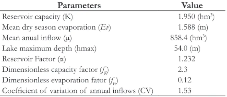
In this study, the reservoir operation rules are deined in function of the releases, evaporation, and spill losses obtained by RTD method (CAMPOS, 2010). Table 4 presents the characteristics of Orós reservoir and the RTD parameters.
Water release rules are set at the beginning of the year, as a function of the hydrological water stored in the reservoir and the forecast inlows in the wet season. In this case, the forecast skill is evaluated using HSS metric. For that, three decisions estimated thresholds in Table 1 were used.
The reservoir operation rules, obtained with the cascade model simulations, were evaluated using the HSS metric. The results were as follows: for release decisions based on VApmed, HSS = 0.55; for release decision based on VArams; HSS = 0.43. The forecast from RAMS/SMA gives good results when used as a tool to predict the seasonal discharges in the Jaguaribe River. It is important to note that these good results were obtained in some high discharge years, such as 1984, 1985, 2004, 2008 and 2009. Therefore, the coupled model give good results in decisions on reservoir operation on a seasonal time scale.
By using RSM 97 and SMAP, in the Jaguaribe River, Alves et al. (2012) obtained HSS = 0.17 without pdf corrections and HSS = 0.27 with pdf corrections, for operation rule decisions. These results corroborate those by Galvão et al. (2005), which showed promising results in the seasonal forecast for a dynamic downscaling of precipitation, along with the rainfall-runoff model and reservoir operation in two watersheds located in Paraiba and Pernambuco.
When forced with observed rainfall data, SMA has a small error (22.5%), whereas when forced by RAMS, even with PDF corrections, SMA has larger errors (39%). These errors can be associated with disabilities (skill) of the atmospheric model to detect some weather systems active in the basin area.
Reservoir operation studies show that the predictions may lead to better operational performance since they allow consideration of all the uncertainties in the future and can serve as input to decision-making models. Such beneits were reviewed, for example, in the works of Boucher et al. (2012), Raso et al. (2013), Fan et al. (2014a, b, 2015a, b), Schwanenberg et al. (2015), Zhao et al. (2011).
CONCLUSIONS
The ability of simulation using the hydrological model SMA proved to be useful to estimate river discharges (NS = 0.87) and thus to improve the decisions on reservoir release rules in semiarid regions.
Although the rainfall dynamic downscaling shows systematic errors in the estimating the rainfall, it presented a better result with the pdf corrections, thereby improving the simulated stream low in the basin of Alto Jaguaribe. The use of seasonal forecast in determination of the volumes stored in the reservoir on a monthly scale from the rainfall model RAMS 6.0 can become an important tool for annual water the allocation in Ceará State.
ACKNOWLEDGEMENTS
The authors thank FUNCEME by data availability.
REFERÊNCIAS
ALVES, J. B.; CAMPOS, J. B.; SERVAIN, J. Reservoir management using coupled atmospheric and hydrological models: the Brazilian semi-arid case. Water Resources Management, v. 26, n. 5, p. 1365-1385, 2012. http://dx.doi.org/10.1007/s11269-011-9963-2.
ALVES, J. M. B.; COSTA, A. A.; SOMBRA, S. S.; CAMPOS, J. N. B.; SOUZA FILHO, F. A.; MARTINS, E. S. P. R.; SILVA, E. M.; SANTOS, A. C. S.; BARBOSA, H. A.; MELCIADES, W. L. B.; MONCUNNIL, D. F. Um estudo inter-comparativo de previsão sazonal estatística dinâmica. Revista Brasileira de Meteorologia, v. 22, n. 3, p. 354-372, 2007. http://dx.doi.org/10.1590/S0102-77862007000300009.
BASHAR, K. E. Comparative performance of soil moisture accounting approach in continuous hydrologic simulation of the Blue Nile. Water Science and Engineering, v. 5, p. 1-10, 2012.
Table 4. Orós data used to deine reservoir release rules. Parameters Value
Reservoir capacity (K) 1.950 (hm3)
Mean dry season evaporation (Ev) 1.588 (m)
Mean anual inlow (µ) 858.4 (hm3)
Lake maximum depth (hmax) 54.0 (m)
Reservoir Factor (α) 1.232
Dimensionless capacity factor (fK) 2.3 Dimensionless evaporation fator (fE) 0.12
Coeficient of variation of annual inlows (CV) 1.53
BENNETT, T. H.; PETERS, J. C. Continuous soil moisture accounting in the Hydrologic Engineering Center Hydrologic Modeling System (HEC-HMS). Water Resources Management, v. 10, p. 1-10, 2000.
BLOCK, P. J.; RAJAGOPALAN, B. Statistical-dynamical approach for streamflow modeling at Malakal, Sudan, on the White Nile River. Journal of Hydrologic Engineering, v. 14, n. 2, p. 185-196, 2009. http:// dx.doi.org/10.1061/(ASCE)1084-0699(2009)14:2(185).
BLOCK, P. J.; SOUZA FILHO, F. A.; SUN, L.; KWON, H.-H. Streamflow forecasting framework using multiple climate and hydrological models. Journal of the American Water Resources Association, v. 45, n. 4, p. 828-843, 2009. http://dx.doi.org/10.1111/j.1752-1688.2009.00327.x.
BOUCHER, M.-A.; TREMBLAY, D.; DELORME, L.; PERREAULT, L.; ANCTIL, F. Hydro-economic assessment of hydrological forecasting systems. Journal of Hydrology (Amsterdam), v. 416-417, p. 133-144, 2012. http://dx.doi.org/10.1016/j.jhydrol.2011.11.042.
CABRAL, S.L.; CAMPOS, J.N.B.; SILVEIRA, C.S.; RODRIGUES, J.M. O intervalo de tempo para uma máxima previsiblidade da precipitação sobre o Semiárido brasileiro. Revista Brasileira de Meteorologia, v. 31, n. 2, 2016.
CAMPOS, J. N. Modeling the yield evaporation spill in the reservoir storage process: the regulation triangle diagram. Water Resources Management, v. 24, n. 13, p. 3487-3511, 2010. http://dx.doi. org/10.1007/s11269-010-9616-x.
CHEN, C.; COTTON, W. R. Numerical experiments with a one-dimensional higher order turbulence model: Simulation of the Wangara day 33 case. Boundary-Layer Meteorology, v. 25, n. 4, p. 375-404, 1983. http://dx.doi.org/10.1007/BF02041156.
CHU, X.; STEINMAN, A. Event and Continuous Hydrologic Modeling with HEC-HMS. Journal of the Irrigation and Drainage, v. 135, n. 1, p. 119-124, 2009. http://dx.doi.org/10.1061/(ASCE)0733-9437(2009)135:1(119).
COLLISCHONN, W. Simulação hidrológica em grandes bacias. 2001. Tese (Doutorado em Engenharia Civil) - Instituto de Pesquisas Hidraulicas, Universidade Federal do Rio Grande do Sul, Rio Grande do Sul, 2001. Disponível em: <http://www.bibliotecadigital.ufrgs. br/da.php?nrb=000320696&loc=2002&l=f46397692f2221cf>. Acesso em: 20 nov. 2015.
COTTON, W. R.; PIELKE SIR, R. A.; WALKO, R. L.; LISTON, G. E.; TREMBACK, C. J.; JIANG, H.; MCANELLY, R. L.; HARRINGTON, J. Y.; NICHOLLS, M. E.; CARRIO, G. G.; MCFADDEN, J. P. RAMS 6.0 2001: Current status and future directions. Meteorology and Atmospheric Physics, v. 82, n. 1, p. 5-29, 2003. http://dx.doi.org/10.1007/s00703-001-0584-9.
CUNGE, J. A. On the subject of a flood propagation computation method (Muskingum Method). Journal of Hydraulic Research, v. 7, n. 2, p. 205-230, 1969. http://dx.doi.org/10.1080/00221686909500264.
DAVIES, H. A lateral boundary formulation for multi-level prediction models. Quarterly Journal of the Royal Meteorological Society, v. 102, n. 432, p. 405-418, 1976.
DOBLAS-REYES, F. J.; HAGEDORN, R.; PALMER, T. N. The reationale behind the success of multi-model ensembles in seasonal forecasting – II. Calibration and Combination. Tellus, v. 57A, n. 3, p. 234-252, 2005. http://dx.doi.org/10.1111/j.1600-0870.2005.00104.x.
FAN, F. M.; COLLISCHONN, W.; MELLER, A.; BOTELHO, L. C. Ensemble streamflow forecasting experiments in a tropical basin: the São Francisco river case study. Journal of Hydrology (Amsterdam), v. 519, p. 2906-2919, 2014a. http://dx.doi.org/10.1016/j.jhydrol.2014.04.038.
FAN, F. M.; COLLISCHONN, W.; QUIROZ, K.; SORRIBAS, M. V.; BUARQUE, D. C.; SIQUEIRA, V. A. Ensemble flood forecasting on the Tocantins River - Brazil. Geofizicheskie Issledovaniia, v. 16, p. 1818, 2014b.
FAN, F. M.; COLLISCHONN, W.; QUIROZ, K.; SORRIBAS, M. V.; BUARQUE, D. C.; SIQUEIRA, V. A. Flood forecasting on the Tocantins River using ensemble rainfall forecasts and real-time satellite rainfall estimates. Journal Flood Risk Management, v. 9, n. 3, p. 278-288, 2015a.
FAN, F. M.; SCHWANENBERG, D.; COLLISCHONN, W.; WEERTS, A. Verification of inflow into hydropower reservoirs using ensemble forecasts of the TIGGE database for large scale basins in Brazil. Journal of Hydrology (Amsterdam), v. 4, p. 196-227, 2015b.
GALVÃO, C. O.; NOBRE, P.; BRAGA, A. C. F. M.; OLIVEIRA, K. F.; SILVA, R. M.; SILVA, S. R.; GOMES FILHO, M. F.; SANTOS, C. A. G.; LACERDA, F.; MONCUNILL, D. Climatic predictability, hydrology and water resources over Nordeste Brazil. Regional Hydrological Impacts of Climatic Change-Impact Assessment and Decision Making. In: IAHS SCIENTIFIC ASSEMBLY, 7., 2005, Foz do Iguaçu. Proceedings… IAHS Publisher, 2005. vol. 295.
GARCÍA, A.; SAINZ, A.; REVILLA, J. A.; ALVÁREZ, C.; JUANES, J. A.; PUENTE, A. Surface water resources assessment in scarcely gauged basins in the north of Spain. Journal of Hydrology (Amsterdam), v. 356, n. 3-4, p. 312-326, 2008. http://dx.doi.org/10.1016/j. jhydrol.2008.04.019.
GEORGAKAKOS, K. P.; BAE, D. H.; JEONG, C. S. utility of ten-day climate model ensemble simulations for water resources applications in korean watersheds. Water Resources Management, v. 19, n. 6, p. 849-872, 2005. http://dx.doi.org/10.1007/s11269-005-5605-x.
GOLIAN, S.; SAGHAFIAN, B.; FAROKHNIA, A. Copula-based interpretation of continuous rainfall-runoff simulations of a watershed in northern Iran. Canadian Journal of Earth Science, v. 49, p .681-691, 2012.
HEIDKE, P. Berechnung der erfolges und der gute der windstarkevorhersagen im sturmwarnungdienst. Geogrfike Annaler, v. 8, p. 301-349, 1926. http://dx.doi.org/10.2307/519729.
KOCH, R.; BENE, K. Continuous hydrologic modeling with HMS in the Aggtelek Karst region. Hydrology, v. 1, p. 1-7, 2013.
KUO, H. L. Further studies of the parameterization of the influence of cumulus convection on large-scale flow. Journal of the Atmospheric Sciences, v. 31, n. 5, p. 1232-1240, 1974. http://dx.doi. org/10.1175/1520-0469(1974)031<1232:FSOTPO>2.0.CO;2.
MELLOR, G.; YAMADA, T. A hierarchy of turbulence closure models for atmospheric boundary layers. Journal of the Atmospheric Sciences, v. 31, n. 7, p. 1791-1806, 1974. http://dx.doi.org/10.1175/1520-0469(1974)031<1791:AHOTCM>2.0.CO;2.
MOLTENI, F.; BUIZZA, R.; PALMER, T. N.; PETROLIAGIS, T. The ECMWF ensemble prediction system: Methodology and validation. Journal of the Royal Meteorological Society, v. 122, n. 529, p. 73-119, 1996. http://dx.doi.org/10.1002/qj.49712252905.
MOURA, A. D.; SHUKLA, J. On the dynamics of drougths in northeast Brazil: observations, theory and numerical experiments with a general circulation model. Journal of the Atmospheric Sciences, v. 38, n. 7, p. 2653-2675, 1981. http://dx.doi.org/10.1175/1520-0469(1981)038<2653:OTDODI>2.0.CO;2.
NASH, J. E.; SUTCLIFFE, J. V. River flow forecasting through conceptual models, Part I: a discussion of principles. Journal of Hydrology (Amsterdam), v. 10, n. 3, p. 282-290, 1970. http://dx.doi. org/10.1016/0022-1694(70)90255-6.
PIELKE, R. A.; COTTON, W. R.; WALKO, R. L.; TREMBACK, C. J.; LYONS, W. A.; GRASSO, L. D.; NICHOLLS, M. E.; MORAN, M. D.; WESLEY, D. A.; LEE, T. J.; COPELAND, J. H. A comprehensive meteorological modeling system-RAMS 6.0. Meteorology and Atmospheric Physics, v. 49, n. 1, p. 69-91, 1992. http:// dx.doi.org/10.1007/BF01025401.
RASO, L.; VAN DE GIESEN, N.; STIVE, P.; SCHWANENBERG, D.; VAN OVERLOOP, P. J. Tree Structure Generation from Ensemble Forecasts for Real Time Control. Hydrological Processes, v. 27, n. 1, p. 75-82, 2013. http://dx.doi.org/10.1002/hyp.9473.
RAUDKIVI, A. J. Hidrology. Oxford: Pergamon Press, 1979. 471 p.
REIS JUNIOR, D. S. Verificação da previsão operacional de chuva sobre Bacias Hidrográficas do Estado do Ceará. In: SIMPÓSIO BRASILEIRO DE RECURSOS HÍDRICOS, 28., 2009, Campo Grande. Anais… Campo Grande: [s.n.], 2009.
SCHWANENBERG, D.; FAN, F. M.; NAUMANN, S.; KUWAJIMA, J. I.; ALVARADO, R.; REIS, A. A. Short-term Reservoir Optimization
for Flood Mitigation under Meteorological and Hydrological Forecast Uncertainty. Water Resources Management, v. 29, n. 5, p. 1635-1651, 2015. http://dx.doi.org/10.1007/s11269-014-0899-1.
SOUZA FILHO, F. A.; LALL, U. Seasonal to interannual ensemble streamflow forecasts for Ceara, Brazil: applications of a multivariate, semiparametric algorithm. Water Resources Research, v. 39, n. 11, p. 1307-1320, 2003. http://dx.doi.org/10.1029/2002WR001373.
SOUZA FILHO, F. A.; LALL, U. Modelo de previsão de vazões sazonais e interanuais. Revista Brasileira de Recursos Hídricos, v. 9, n. 2, p. 61-74, 2004. http://dx.doi.org/10.21168/rbrh.v9n2.p61-74.
SUN, L.; MONCUNILL, D. F.; LI, H.; MOURA, A. D.; SOUZA FILHO, F. A. Climate downscaling over Nordeste, Brazil, Using the NCEP RSM97. Journal of Climate, v. 18, n. 4, p. 551-567, 2005. http://dx.doi.org/10.1175/JCLI-3266.1.
THIESSEN, A. H. Precipitation averages for large areas. Monthly Weather Review, v. 39, p. 1082-1089, 1911.
TOTH, Z.; KALNAY, E. Ensemble forecasting at NMC: the generation of perturbations. Bulletin of the American Meteorological Society, v. 74, n. 12, p. 2317-2330, 1993. http://dx.doi.org/10.1175/1520-0477(1993)074<2317:EFANTG>2.0.CO;2.
UVO, C. B. T. U.; BERNDTSSON, R. Forecasting discharge in Amazonia using artiicial neural networks. International Journal of Climatology, v. 20, p. 1495-1507, 2000. http://dx.doi.org/10.1002/1097-0088(200010)20:12<1495::AID-JOC549>3.0.CO;2-F.
WALKO, R.; COTTON, W. R.; MEYERS, M. P.; HARRINGTON, J. Y. New RAMS 6.0 cloud microphysics parameterization Part I: the single-moment scheme. Atmospheric Research, v. 38, n. 1, p. 29-62, 1995. http://dx.doi.org/10.1016/0169-8095(94)00087-T.
ZHAO, T.; XIMING, C.; DAWEN, Y. Effect of streamflow forecast uncertainty on real-time reservoir operation. Advances in Water Resources, v. 34, n. 4, p. 495-504, 2011. http://dx.doi.org/10.1016/j. advwatres.2011.01.004.
Authors contributions
Samuellson Lopes Cabral: paper conception, bibliographical research, data analysis, calibration and validation of SMA, analysis and discussion of the results and preparation of the text.
José Nilson Bezerra Campos: paper conception, analysis and discussion of the results and preparation of the text.