Reservoir Management Using Coupled Atmospheric
and Hydrological Models: The Brazilian Semi-Arid Case
José Maria Brabo Alves&José Nilson B. Campos&
Jacques Servain
Received: 4 August 2010 / Accepted: 22 December 2011 / Published online: 11 January 2012
#Springer Science+Business Media B.V. 2012
Abstract This study investigated the sensitivity of a dynamic downscaling atmospheric model system coupled with a rainfall-runoff model to hindcast an example of reservoir water management in the semi-arid region of Northeast Brazil (NEB). A regional atmospheric spectral model (RSM) is driven by the outputs of an atmospheric general circulation model (AGCM), itself forced by the observed sea surface temperature over the World Ocean. Daily precipitation simulated by the RSM was then used as the input to a hydrological rainfall-runoff model for the Upper Jaguaribe River Basin to estimate inflows at the Orós Reservoir in the state of Ceará. A hindcast analysis of precipitation was performed during the rainy season over NEB (January to June) from 1971 to 2000. The RSM captured the precipitation variability relatively well when a probability density function (PDF) was used to correct the numerical bias. Three hindcast series of inflow using (i) the observed rainfall, (ii) the simulated rainfall before the PDF correction, and (iii) the simulated rainfall after the PDF correction were performed during the study period and then compared to the series of observed inflow. The atmospheric-rainfall-runoff“cascade”model efficiency was evaluated by comparing the Orós Reservoir release decisions from different scenarios based on observed, simulated (RSM, RSM-PDF), and mean historical reservoir inflows. The cascade model has the potential, relatively well balanced during dry, normal or wet years, to be a
DOI 10.1007/s11269-011-9963-2
J. M. B. Alves (*)
Fundação Cearense de Meteorologia e Recursos Hídricos (FUNCEME), Av. Rui Barbosa 1246, Aldeota, 60115-221 Fortaleza, CE, Brazil
e-mail: brabo@funceme.br
J. N. B. Campos
Departamento de Engenharia Hidráulica e Ambiental - Centro de Tecnologia, Universidade Federal do Ceará (UFC), Fortaleza, Ceará, Brazil
J. Servain
Institut de Recherche pour le Développement (IRD), UMR-182, Paris, France
Present Address:
J. Servain
useful tool to correctly forecast the decision managements of reservoirs in the semi-arid region of NEB. Additional progress in the numerical simulation is however necessary to improve the performance.
Keywords Discharge simulation . Downscaling atmospheric model . Hydrological modeling . Reservoir management . Northeast Brazil . Semi-arid regions
1 Introduction
Dynamic atmospheric general circulation models (AGCMs) at global scale, and atmospheric regional models (RMs) at regional scales, have become useful for forecasting the weather and climate in many regions around the world (Sun et al. 2005). The spatial resolution of the AGCMs is relatively coarse (2.5×2.5°) and these models are generally unable to resolve sub-grid characteristics, such as detailed cloud cover, local topography, and land surface conditions (Tisseuil et al.2010). These variables are more accurately resolved by the RMs where the spatial resolution is about 0.5×0.5°, i.e., 60 km×60 km (Cocke and La Row2000).
The downscaling approach, using in sequence an AGCM and a RM, makes it possible to combine a large-scale environment forcing with a small-scale resolution of the atmospheric variables over a determined area. There are two main types for downscaling large AGCM outputs into a finer spatial resolution. A first type is the statistical downscaling that uses the statistical relationship between the AGCM resolution climate variables and the local climate (e.g., Fowler et al.2007). A second type is the regular dynamic downscaling, where AGCM data are used to input into regional models (e.g., Sun et al.2005). There are advantages and disadvantages to each type (Fowler et al.2007; Dibike and Coualibaly2005). The statistical downscaling uses transfer functions for regression analyses in addition to a neural network (Hewitson and Crane1996). It is computationally efficient and comparatively inexpensive compared to the dynamic process. However, it requires long periods of reliable historical data for calibration and depends on the choice of predictors (Fowler et al.2007).
The dynamic downscaling presents good performance for atmospheric variable config-urations and intensities on the regional scale where AGCMs have poor sensitivity (Giorgi 1990; Nobre et al.2001; Sun et al.2005). Though the final outputs are strongly dependent from AGCM boundary forcing, they are based on physically consistent processes and have a finer resolution (Fowler et al.2007). This downscaling process is especially interesting in semi-arid regions where the performance of the local precipitation distribution is improved (Nobre et al.2001; Sun et al.2005; Marengo2005). Indeed, this technique has already been tested for some drainage basins in Northeast Brazil (NEB) (Silva Filho2005; Cardoso et al. 2005; Galvão et al.2005), where these previous works were mainly performed to study the dynamic response for monthly climatic averages (Sun et al.2005). In the present study we used such a dynamic downscaling system at intra-monthly timescale.
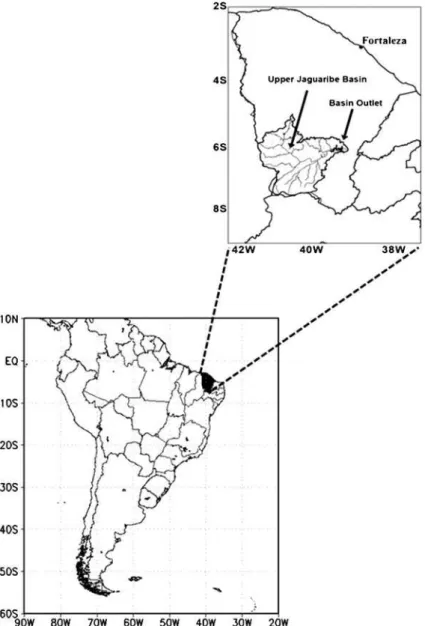
In this study, the outputs of an AGCM (ECHAM 4.5; Sun et al.2005) for the period 1971– 2000 were used to feed a RM (RSM-97; Juang and Kanamitsu1994) operating over the Upper Jaguaribe River Basin in Ceará State (Fig.1). The analysis of the simulated daily precipitation was limited to the wet season, January to June, which represents more than 90% of the annual precipitation over NEB (Uvo et al.1998). This simulated precipitation was used to estimate the daily Upper Jaguaribe River Basin discharge using the Soil Moisture Accounting Procedure (SMAP) (Lopes et al.1981). These variables were then integrated at different intra-monthly periods (1-day, 5-day, and 15-day periods) and ultimately used to hindcast the inflow volumes in the Orós Reservoir located at the Upper Jaguaribe River Basin outlet.
Fig. 1 Map of South American (left) with a magnified region showing Ceará State and the Upper Jaguaribe
2 Climate and Hydrological Characteristics of the Area of Interest
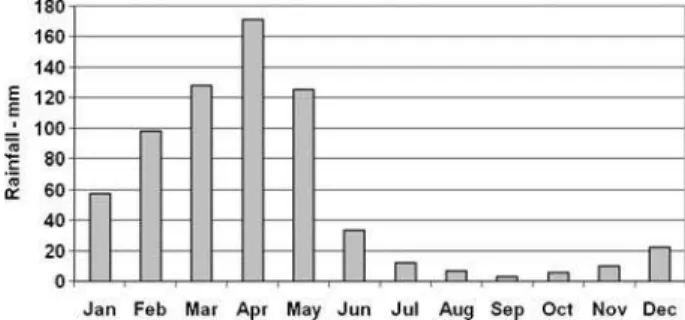
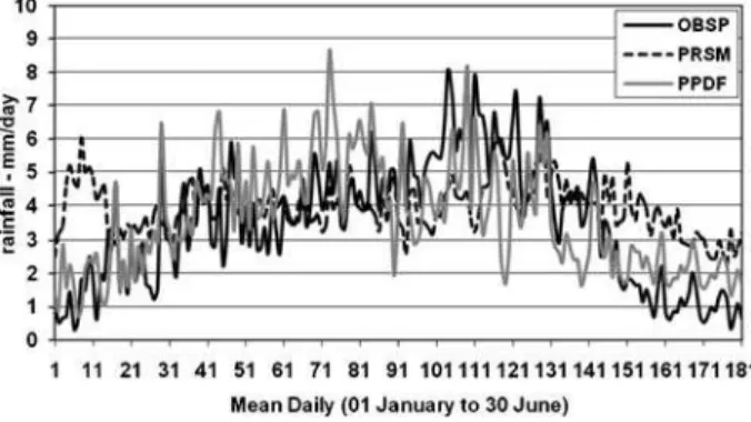
NEB is a semi-arid region where most of the streams are seasonally intermittent and the principal sources of fresh water for the local population are provided by surface reservoirs. Ceará State is located in the northern part of NEB between latitudes 3°S and 8°S and longitudes 37°W and 41°W and has a surface of 146,300 km2(Fig.1). The annual rainfall in Ceará ranges from 500 mm in the inland plains (i.e., Upper Jaguaribe River Basin) to about 1400 mm along the Atlantic coast and over the high reliefs (600–1000 m altitude). The rainfall pattern in northern NEB is clearly marked by two seasons. The wet season occurs during the first 6 months of the year, with a pre-rainy season in January and a post-rainy season in June. The dry season with little or no precipitation occurs during the remainder of the year (Fig. 2). The core of wet season (February-to-May) is directly linked to the meridional seasonal migration of the inter-tropical convergence zone (ITCZ) over the Atlantic Ocean, which reaches its southernmost position within the latitudes of the northern NEB at this time of the year (Uvo et al.1998). Pre- and post-rainy seasons are mainly linked to local transient atmospheric disturbances (Barreiros and Chang2002).
Evaporation inland in Ceará reaches more than 2,500 mm per year. In a normal year, the water budget, i.e., precipitation minus evaporation is only positive for 3 to 4 months during the wet season. These severe climatic conditions, coupled with a crystalline soil and low underground storage capacity, result in intermittent rivers. Thus, rarely the rivers in Ceará have discharges after June. They remain dry for 6 to 9 months per year or even for more than 1 year if a severe drought occurs (Campos and Studart2008).
To prevent the intermittency of rivers and recurrent droughts, the Brazilian Federal Govern-ment built many reservoirs at the beginning of the 20th Century to ensure a sufficient supply of fresh water for the local population during the dry seasons and drought years. The Orós Reservoir was built in 1965 in the context of that policy. Orós has a capacity of 1.95 billion cubic meters and is located at the Upper Jaguaribe River Basin outlet (Fig.1). The Orós Reservoir therefore plays an important role in decisions about water management in Ceará State. One of these decisions is, for instance, whether to transfer fresh water from the Orós Reservoir to the city of Fortaleza, which is the capital of Ceará State (Fig.1) and homes to 3.5 million people. Such decisions about water transfer are generally made at the beginning of the year (January–February) and at the end of the wet season (June). In the first case, the decision maker does not know how much water will come during the wet season; in the second case, the decision maker knows that no significant rainfall will come during the next 6 months and has to decide how to use the stored water until the next wet season. Thus, only the months from January to June were analyzed in this paper.
The whole Jaguaribe River extends for about 610 km, and its drainage basin covers 76,000 km2 in surface representing almost half of Ceará State
’s territory (Fig. 1). The observed hydrological regime of that basin is described here by the discharges recorded at
Fig. 2 Monthly averages (1971–
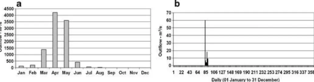
the Iguatu fluviometric station, which covers 24,000 km2 of drainage area, including the 2000 km2controlled by the Trussu Reservoir on the right margin of the Jaguaribe River. The discharge in the Upper Jaguaribe River Basin at Iguatu station was considered in this study to be the only Orós inflow. Its seasonal discharges ranged from zero to 7,000 m3/s with monthly values that are only important in March, April, May and June (Fig.3a). Figure3billustrates an example of a dramatic hydrological drought that occurred during 20 months from July 1957 to March 1959. During that drought period, the Jaguaribe River stayed dry except for 5 days at the end of March 1958, when the maximum daily discharge reached 60 m3/s.
3 Hydrological Data Sets and Methodology 3.1 Hydrological Data Sets
Hydrological data measured in the Upper Jaguaribe River Basin are available since 1908, when precipitation and streamflows observation networks were installed across the NEB by theDepartamento Nacional de Obras Contra as Secas (DNOCS).There are now 108 rain gauges operating in this area, all monitored by Fundação Cearense de Meteorologia e Recursos Hídricos (FUNCEME)and available atwww.funceme.br. However, only the data sets for 64 stations passed the consistency tests performed by Xavier et al. (2000). Using the Thiessen polygon method, the observed daily precipitation was integrated over the Upper Jaguaribe River Basin during the first 6 months of the period 1971–2000. A time series representing the mean daily precipitation over the basin was obtained and used as the observed daily rainfall in the cascade model system which is described herafter.
The Jaguaribe River Basin discharges are recorded by a fluviometric station located at Iguatu (Fig.1), outlet of basin. Data collection and data consistency are routinely reviewed by the Agência Nacional de Águas (ANA) and are available at www.ana.gov.br. The observed daily discharges are available from 1921 to 2010 with some missing data.
3.2 Methodology
The numerical models used in this paper are presented in the following four sub-sections: (i) the atmospheric coupled model system (AGCM+RM) used to simulate the daily precipitations over NEB; (ii) the rainfall-runoff model (SMAP) which used the observed and simulated daily precipitation as inputs to estimate the daily streamflows; (iii) the reservoir operation model that used different realizations of river streamflows to guide decisions about the reservoir water releases; and finally, (iv) the“cascade”model described as a whole.
3.2.1 Atmospheric Models
The AGCM ECHAM-4.5 was initially developed at the European Center for Medium Range Weather Forecasts (ECMWF) (Roeckner1996). Some modifications in the physics of the model were applied at the Max-Planck Institute for Meteorology and the German Climate Computing Centre (DKRZ) to improve the consistency of the climatic outputs. The regional model, RSM-97, which was developed at the National Center for Environment Prediction (NCEP) (Juang and Kanamitsu1994), is now routinely run atFUNCEME.
According to Sun et al. (2005), ECHAM-4.5 was driven by a sea surface temperature (SST) data set collected between 1971 and 2000, called the Excellent Interpolation data set, and prepared at the International Research Institute for Climate and Society (IRI) (Reynolds and Smith1994). To obtain a larger set of realizations (Sun et al.2005) ECHAM-4.5 was run using ten distinct initial conditions. These AGCM outputs were subsequently used to drive ten RSM-97 realizations (Fig.4). In this study, the average of these RSM-97 outputs was used to focus on the seven grid steps (60 km×60 km) covering the Upper Jaguaribe River Basin. The daily precipitation during the first six-month periods of 1971–2000 was inte-grated over these seven grid steps and compared with the observed daily rainfall recorded by the Iguatu station rain gauge.
The application of RSM-97 for daily precipitation introduces a bias on the simulated values, as observed by Feddersen et al. (2004). To remove this bias, some techniques are available in the literature. In this paper, we used the Probability Density Function (PDF) technique (Mukhopadhyay et al.2010). This technique consists of building a curve using the observed precipitation series data. For this method, the observed values are obtained from a different period than that of the simulated values. In our case, the observed time series from 1940 to 1970 was used to correct the RSM simulated series from 1971 to 2000.
The data were used as follows: 1) observed precipitations were used to build the PDF curve for removing the biases for the period 1940–1970; 2) observed precipitations and
observed discharges were used to calibrate (1950–1960) and validate (1961–1970) the SMAP parameters (see next section); 3) observed and simulated (without and with PDF correction) precipitation, and observed and simulated (without and with PDF correction) discharges were used for the cascade model for the period 1971–2000. Thus, all of the calibration and corrections were derived from observations outside of the period of application of the cascade model.
3.2.2 Rainfall-Runoff Model
SMAP (Lopes et al.1981), the model used here to generate the daily runoff from the daily rainfall, is currently applied at FUNCEME for hydrological studies and water resources management in the state of Ceará. SMAP uses two linear reservoirs to represent the surface reservoir (soil surface layer) and the underground reservoir. For each precipitation event (P), the water balance is evaluated, and a parcel of P is transferred to the surface reservoir, which is estimated using the Soil Conservation Service TR_55 procedure. The remaining parcel is divided between evaporation and infiltration.
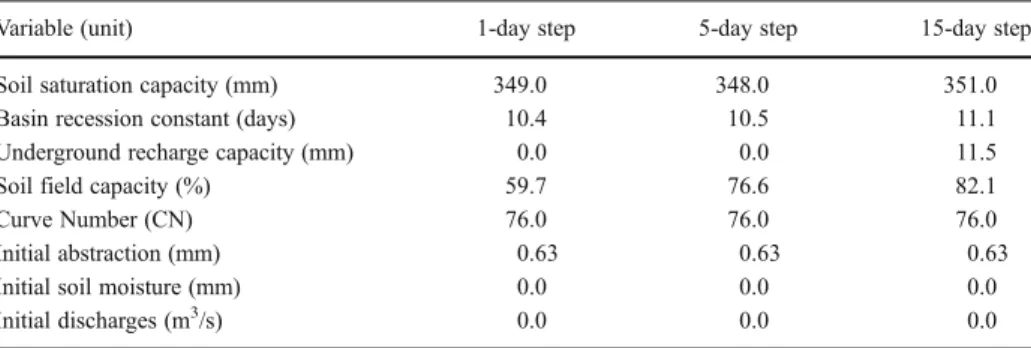
SMAP needs eight parameters (Table1) to evaluate the water budget and to estimate the river discharges at the basin outlet. Two parameters are computed from basin physical characteristics: (i) the National Research Conserve Service (NRCS) curve number (CN) derived from land use, vegetation cover, soil classification, hydrologic conditions and antecedent runoff conditions, and (ii) the initial abstraction as function of CN in the standard coefficient recommended by NRCS (Ponce, 1989). Two other parameters are arbitrated as zero from hydrological and climate peculiarities of the region: (i) the initial discharge, and (ii) the initial soil moisture. The four remaining parameters, i.e., (i) the soil saturation capacity, (ii) the basin recession constant, (iii) the underground recharge capacity, and (iv) the soil field capacity, must be calibrated. This calibration was accomplished here using the Nash-Sutcliffe efficiency (NSE) coefficient (Nash and Suctcliffe1970) for precipitation and runoff at 1-day, 5-day and 15-day time scales for the 1951–1960 period, while the validation was performed using the 1961–1970 period. This NSE between the simulated and observed outflows was calculated using the following equation:
NSE¼1
Pn
t¼1 xt yt
ð Þ2
Pn
t¼1ðxt xÞ
2 ð1Þ
Table 1 Values of the calibrated (lines 1 to 4) SMAP parameters using the NSE, and values of the estimated (lines 5 to 8) SMAP parameters for the Upper Jaguaribe River Basin
Variable (unit) 1-day step 5-day step 15-day step
Soil saturation capacity (mm) 349.0 348.0 351.0
Basin recession constant (days) 10.4 10.5 11.1
Underground recharge capacity (mm) 0.0 0.0 11.5
Soil field capacity (%) 59.7 76.6 82.1
Curve Number (CN) 76.0 76.0 76.0
Initial abstraction (mm) 0.63 0.63 0.63
Initial soil moisture (mm) 0.0 0.0 0.0
where xand y denote, respectively, the daily observed and simulated (RSM-97 corrected with PDF) precipitation from January 1 to June 30, and x represent the observed precip-itations averaged during 1971–2000. The NSE was 0.46, 0.45 and 0.50 for the calibration series and 0.40, 0.42 and 0.46 for the validation series at 1-day, 5-day and 15-day timescales respectively. The values of the four estimated and the four calibrated SMAP parameters are given in Table1.
3.2.3 Reservoir Operation Model
The reservoir yield, denoted by Y, is the amount of water to be released from the reservoir whenever there is availability. The reservoir release at time t (Rt) is the water volume
effectively liberated from the reservoir to meet the demand. Thus, theRtvalues are equal
to or less than Y and depend on the reservoir water content.
The simulated reservoir operation was performed using the following budget equation:
Siþ1¼SiþðPi EiÞ Aiþ1þAi
2
þIi Ri; ð2Þ
whereSiandSi+1(m3/s) denote the daily reservoir storage at times t and t+1, respectively;
Pi(m/day) and Ei (m/day) represent, respectively, the mean daily precipitation, and the
mean daily evaporation rate over the reservoir surface at time i; Ai and Ai+1 (m2) are the
reservoir area at times t and t+1, respectively;Ii(m3/s) andRi(m3/s) are the inflow and the
reservoir release at time I, respectively.
The yield for the hydrological regime in NEB can be estimated using the regulation triangle diagram (RTD). This method is a graphical solution of the reservoir budget equation in its dimensionless form (Campos 2010) and estimates the expected value of releases, evaporation and spills. It is mainly based on two dimensionless parameters: the evaporation factor (fE) and the reservoir capacity (fK). The evaporation factor was estimated by:
fE¼3E
a1=3
μ1=3 ; ð3Þ
where αindicates a reservoir of dimensionless shape; Eis the reservoir evaporation rate
during the dry season, andμis the mean annual reservoir inflow estimated using the wet
season data. Theαvalue was estimated by:
a¼ K
hmax
ð Þ1=3; ð4Þ
where K is the reservoir capacity and hmax indicates the maximum water depth for the
reservoir. The dimensionless capacity was calculated, with all variables previously defined, as:
fk ¼K
μ ð5Þ
Hereafter are the values of the main Orós Reservoir physical characteristics such as they were used in our experiments:
& Reservoir capacity (K)01,950.0 hm3
& Mean annual reservoir inflow (μ)0858.4 hm3 & Maximum water depth (hmax)054.0 m
& Reservoir shape factor (α)012.32 (computed with Eq.4)
& Dimensionless reservoir capacity (fK)02.30 (estimated with Eq.5) & Dimensionless evaporation factor (fE)00.12 (estimated with Eq.3) & Coefficient of variation of annual inflows (Cv)01.53
The analysis was performed using the following different reservoir inflow data sets:
& Observed reservoir inflows (these are used as a reference to evaluate the decisions); & Reservoir inflows estimated by SMAP forced by the observed precipitations;
& Reservoir inflows estimated by SMAP forced by the RSM-97 precipitations without
PDF correction;
& Reservoir inflows estimated by SMAP forced by the RSM-97 precipitations corrected by
PDF.
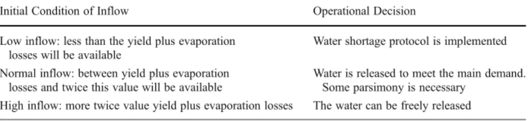
The efficiency of the model was evaluated by comparing the really observed inflows (1971–2000) with the inflows simulated according to the previously discussed hindcast scenarios. Table 2 summarizes the scenarios of operational decisions for the reservoir management of the Orós reservoir according to different conditions of initial inflows (low, normal and large inflows).
3.2.4 Cascade Model
The cascade model can be synthesized as shown in Fig. 4. The AGCM, forced by the global observed SST during 1971–2000, generated a first series of ten sets of daily precipitation in low space resolution. These AGCM outputs drove the RSM-97 to obtain a second series of ten sets of daily precipitation over the NEB at a higher space resolution. Then, the both averages (i.e., before and after PDF correction) of this second series of ten sets were used to represent two independent sets of the expected values of daily precipitation over the Upper Jaguaribe River Basin. These two sets of simulated precipitation, as well as the set of observed precipitation, were then used to force the rainfall-runoff model (SMAP) in order to generate three sets of modeled discharge values that feed the Orós reservoir in Ceará State. These three sets of simulated inflow were compared to the set of observed inflow. Finally, the five reservoir operation decisions using observed, simulated (three experiments) and climatic inflows, were compared. The Heidke Score Skill (Eq.6) was used to measure the efficiency of the model system during the period 1971–2000.
Table 2 Scenarios and operational decisions for the reservoir management according to different initial inflows
Initial Condition of Inflow Operational Decision
Low inflow: less than the yield plus evaporation losses will be available
Water shortage protocol is implemented
Normal inflow: between yield plus evaporation losses and twice this value will be available
Water is released to meet the main demand. Some parsimony is necessary
4 Results and Discussion
The results were analyzed according to the three steps discussed above: (i) observed and RSM-97 simulated precipitation (with and without PDF correction); (ii) observed and estimated (using or not PDF correction for RSM-97 precipitation) discharge; and (iii) comparison of reservoir management decisions using observed, estimated (using or not PDF correction for the precipitation and using the observed precipitation) and climatic averages of discharges.
4.1 Observed and Simulated Precipitation
Figure5shows three sets of daily precipitation (in mm/day) for the first semesters averaged during 1971–2000. The sets include the observed precipitation (OBSP), the precipitation simulated by RSM-97 before PDF correction (PRSM), and the precipitation simulated by RSM-97 after PDF corrections (PPDF). All three sets show an important increase in precipitation during the core of the rainfall season (>5 mm/day between February and May). In addition, the PRSM time series was significantly different from the observed precipitation (OBSP). Indeed, RSM-97 overestimated the precipitation by 3–4 mm/day during the beginning and the end of the rainfall season, while it underestimated the precipitation by about 2 mm/day in April, i.e., during the core of the seasonal rainfall in NEB. Thus, the correlation between these variables was low (r0+0.13). After the PDF
correction, the PPDF values were closer to OBSP, especially during the first weeks of the year when the OBSP and PRSM time series were very different. The improvement is less efficient in June. The correlation coefficient between OBSP and PPDF became r0+0.63.
This result encouraged us to use the simulated daily rainfall to estimate the daily discharge through the SMAP. The parameters were calibrated according to the procedure described previously. As it can be seen in Fig. 5, the total variability of the precipitation simulated by the not-corrected RSM-97 (Root Mean Square Error, RMSE00.73 mm/day)
was about half of this value for the observations (RMSE01.89 mm/day), while it was much
higher (RMSE06.20 mm/day) for the RSM-97 precipitation corrected with PDF. Several
possible factors may be responsible for these differences. For the RSM-97 without correc-tion, there was evidence of weak performance concerning the parameterization of convec-tion (Nobre et al.2001). This resulted in a poor simulation of large rainfall episodes and thus reduced the variability. In the case of the simulated rainfall corrected with PDF, the more intense daily precipitation occurrences, although not frequent, had a greater influence on the variability.
Fig. 5 Mean daily precipitation
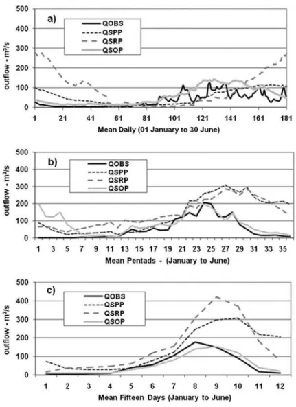
4.2 Observed and Estimated Discharges
Figure6shows the discharge on the Upper Jaguaribe River Basin integrated according to 1-day (top), 5-day (middle) and 15-day (below) timescales and averaged for the first semesters from 1971 to 2000. Four curves represent the observed discharge (QOBS), the discharge estimated by SMAP driven by the observed precipitation (QSOP), the discharge estimated by SMAP driven by RSM-97 precipitation before PDF correction (QSRP), and the discharge simulated by SMAP driven by RSM-97 precipitation after PDF correction (QSPP). Except for January in the 5-day analysis, where an overestimation of about
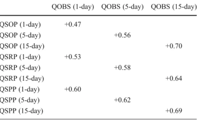
100 m3/s was noted, the discharge computed by SMAP from the observed daily rainfall (QSOP) was very close to the observed discharge (QOBS).The SMAP simulated discharge driven by RSM-97 precipitation was relatively correct during the period from January to April, especially when the PDF technique was used. The results were, however, poor by the end of the semester, especially in May when the estimated daily discharge (driven by not-corrected precipitation) was overestimated by approximately 250 m3/s (i.e., almost twice the observed values). However, the PDF correction was particularly efficient for the 15-day scale, where the discharge error was reduced to an overestimation of 150 m3/s in May. Table3 gives integrated information describing how well the simulated discharges of the Upper Jaguaribe River Basin at the different time steps match the observed values. In this table, the correlation coefficient between observed and simulated inflows increased in all scales when the PDF corrected value of precipitation was used.
4.3 Reservoir Management Decisions
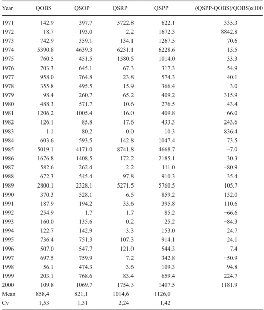
The efficiency of the cascade model for the water reservoir decision was evaluated for the period 1971–2000 using the Orós’s inflow database. Table4shows the observed (QOBS) and estimated (QSOP, QSRP and QSPP) values for the 15-day scale of the Orós Reservoir inflow accumulated during the wet season for all the years 1971 to 2000. The last column of Table4indicates also the relative percent difference (in%) between QSPP and QOBS for each year. The Nash-Sutcliffe model efficiency coefficients between QOBS values and other variables were calculated. Obviously, the QSOP vs. QOBS coefficient is the higher (0.93), and the QSRP vs. QOBS coefficient is the worst (−0.26). The QSPP vs. QSOB coefficient is relatively high (0.67) and represents a general good agreement between corrected-simulations and observations values. That was indeed the case for some years, as for instance in 1978 with a small relative percent difference QSPP-QOBS of +3.0% (Table4). But for some other years the difference between simulated and observed inflows was very large and positive, as for instance in 1972 with a relative percent difference of +8842.8%, or in 2000 with a relative percent difference of +1181.9%.
Why such large differences sometimes? Table5illustrates our hypotheses to explain that problem. It shows the observed (OBSP) and estimated-corrected (PPDF) mean daily pre-cipitation during the months January to June for the three cases pointed before (1972, 1978 and 2000). It can be inferred from Table5that the great differences noted between simulated and observed accumulated outflows were associated to over-estimation by the atmospheric model system of the precipitation during pre- or (especially) post-rainy seasons (see Fig.3a
Table 3 Correlation coefficients between the observed and simulated discharges of the Jaguaribe River at the Iguatu outlet averaged from 1971 to 2000 during the first six-month periods of each year, grouped in 1-day, 5-day and 15-day time-scales. The correlation coefficients up to |0.33| were statistically signif-icant at the 95% level according to the second Student’st-test. See the legend of Fig.6for the definition of the acronyms
QOBS (1-day) QOBS (5-day) QOBS (15-day)
QSOP (1-day) +0.47
QSOP (5-day) +0.56
QSOP (15-day) +0.70
QSRP (1-day) +0.53
QSRP (5-day) +0.58
QSRP (15-day) +0.64
QSPP (1-day) +0.60
QSPP (5-day) +0.62
for the monthly average example). This characteristic was verified in 1972 (see Table5) when the PPDF-OBSP difference was +29.65 mm/day in January whereas the average of that difference for the five following months was only +2.36 mm/day. That was also the case in 2000 (see Table5) when the PPDF-OBSP difference 11.75 mm/day in June whereas the average of that difference for the five previous months was 2.29 mm/day, thus significantly smaller. Based on the whole 30 years period of the experiment, we found that for 60% of the years the precipitation in June overestimated, at minimum, 30% of the observation value. Conversely, the 1978 year, i.e., when the corrected-estimated (QSPP) and observed (QOBS) values of the Orós Reservoir inflow accumulated during the wet season were close (see Table 4 Observed and estimated Orós Reservoir inflow (hm3) during the wet season from 1971 to 2000. See the legend of Fig.6for the definition of the acronyms. The two last lines are related to the mean and the coefficient of annual variation of reservoir inflow (Cv) averaged during the 30 years 1971–2000
Year QOBS QSOP QSRP QSPP (QSPP-QOBS)/QOBS)x100
1971 142.9 397.7 5722.8 622.1 335.3
1972 18.7 193.0 2.2 1672.3 8842.8
1973 742.9 359.1 134.1 1267.5 70.6
1974 5390.8 4639.3 6231.1 6228.6 15.5
1975 760.5 451.5 1580.5 1014.0 33.3
1976 703.3 645.1 67.3 317.3 −54.9
1977 958.0 764.8 23.8 574.3 −40.1
1978 355.8 495.5 15.9 366.4 3.0
1979 98.4 260.7 65.2 409.2 315.9
1980 488.3 571.7 10.6 276.5 −43.4
1981 1206.2 1005.4 16.0 409.8 −66.0
1982 126.1 85.8 17.6 433.3 243.6
1983 1.1 80.2 0.0 10.3 836.4
1984 603.6 593.5 142.8 1047.4 73.5
1985 5019.1 4171.0 8741.8 4668.7 −7.0
1986 1676.8 1408.5 172.2 2185.1 30.3
1987 582.6 262.4 2.2 111.0 −80.9
1988 672.3 545.4 97.8 910.3 35.4
1989 2800.1 2328.1 5271.5 5760.5 105.7
1990 370.3 528.1 6.5 859.2 132.0
1991 187.9 194.2 33.6 395.8 110.6
1992 254.9 1.7 1.7 85.2 −66.6
1993 160.0 135.6 0.2 25.2 −84.3
1994 122.7 142.9 3.3 153.0 24.7
1995 736.4 751.3 107.3 914.1 24.1
1996 507.0 547.7 121.0 544.3 7.4
1997 697.5 759.9 7.2 342.8 −50.9
1998 56.1 474.3 3.6 109.3 94.8
1999 203.1 768.6 83.4 659.4 224.7
2000 109.8 1069.7 1754.3 1407.5 1181.9
Mean 858,4 821,1 1014,6 1126,0
Table4), is a example of relatively good estimation of the precipitation: the average of the difference PPDF-OBSP for the full six-month rainy season was only 1.55 mm/day. Now, how to explain such overestimation of the simulated precipitation during the pre- or post-rainy season? A possible explanation could come from the difference in the causes of the precipitation over NEB during pre- (i.e., January), core- (i.e., February–May), and post- (i.e., June) rainy seasons. During the core rainy season, like that was already indicated in Section 2, the precipitation over NEB is directly controlled by the meridional seasonal migration of the ITCZ, which is also a zone of maximum of precipitation over the Ocean and the adjacent continents. Because this ITCZ latitudinal migration is itself directly associated to the large SST variability over the tropical Atlantic, and because, in our experiment, the precipitation over NEB is simulated by an atmospheric model system itself forced by observed SST, that explains the relative good consistency between simulation and observation of the precipita-tion during that core rainy period. In contrast, during the pre- and (especially) post-rainy seasons, when the ITCZ is more distant from the NEB, rare (but sometimes strong) precipitation episodes over NEB are not caused by large basin-scale SST variability, but are mainly the consequences of local and regional transient disturbances of the atmospheric circulation (Barreiros and Chang 2002). These atmospheric disturbances include frontal systems, cyclonic vortices at high level, and easterly waves crossing the equatorial basin (Kousky1979; Kousky and Gan1981). Such overestimation in the present experiment was probably caused by a default in the parameterization of atmospheric transient processes linked to these local rainy events (Sun et al.2005). Another factor candidate to explain the worst PPDF values of Table4could come from erroneous values of the daily evaporation used in the SMAP model. In fact, since there does not exist any record of observed evaporation in the Upper Jaguaribe basin during the period of experiment (1971–2000), we used evaporation values daily interpolated from an historical monthly data base of evaporation which was daily observed from a class tank at Iguatu meteorological station during the period 1961–1990.
Interesting variations can be noted in the statistical characteristics related to the different inflow realizations. For instance, looking back at Table4, the mean inflow simulated with recorded precipitation (QSOP) is slightly weaker (4.3%) than the mean observed inflow (QOBS) averaged during the same period 1971–2000 (821.1 vs. 858.4 hm3). In parallel, the coefficient of variation of reservoir annual inflow (Cv) decreases from 1.53 to 1.31. For Table 5 Observed and estimated precipitation (mm/day) during the wet season (from January to June) in the Upper Jaguaribe River Basin at Iguatu. See the legend of Fig.5for the definition of the acronyms. DIF signifies the PPDF-OBSP difference
JAN FEB MAR APR MAY JUN
1972 (PPDF) 29.65 5.43 2.09 1.25 1.39 2.46
1972 (OBSP) 0.00 0.41 0.07 0.02 0.30 0.00
DIF (PPDF-OBSP) 29.65 5.02 2.02 1.23 1.09 2.46
1978 (PPDF) 2.36 0.93 0.82 0.96 1.95 2.28
1978 (OBSP) 0.05 1.92 2.38 0.82 3.25 0.65
DIF (PPDF-OBSP) 2.31 −0.99 −1.56 0.1 −1.30 1.63
2000 (PPDF) 2.01 1.33 4.56 2.40 3.88 11.83
2000 (OBSP) 0.00 0.32 1.17 0.81 0.43 0.08
these two realizations, the shapes of the histogram analysis (i.e., inflow frequency in function of inflow class values) are quite similar, as that can be illustrated on Fig.7(top panels). Indeed, for both realizations QOBS and QSOP, similar high values of frequency (~ 15%) are noted in the left part of the panels (what corresponds to rather low values of inflow, less than 2000 hm3), while low values of frequency (<2%) spread out within inflow up to 5000 hm3. The comparisons of the statistical characteristics between the full simulated realizations (QSRP and QSPP) and the observed inflow (QSOP) are quite different. The 1971–2000 mean inflow increases by 18.7% from QOBS to QSRP (1014.6 vs. 858.4), while the Cv coefficient increases from 1.53 to 2.24. This high Cv value of QSRP results in a very different behavior of the frequency inflow diagram (left bottom panel of Fig.7). For that case, i.e., before the PDF correction, the model system concentrates in an erroneous way (~ 24%) the inflow frequency within the very low values (at left), and stretches, also in an erroneous way, the inflow frequency within high values (at right) up to 9000 hm3. After the PDF corrections, the model system increases in 31.8% the mean inflow (QSPP) compared with that variable calculated from the QOBS experiment, which is a larger rise than from QOBS to QSRP experiments. On the other hand, Cv goes down from 1.53 (QOBS) to 1.42 (QSPP), which is an intermediate value between QOBS’s Cv and QSOP’s Cv. That quite positive result is illustrated in the right bottom panel of Fig.7, where it can be noted that the shape of the frequency inflow associated to QSPP is quite similar with those of QOBS and QSOP frequency diagrams. That means that the PDF technique corrects relatively well the comportment of the empirical distribution function but does not remove sufficient the bias in the total average. As that will be shown later by the contingency analysis (see Tables9and 10), these variations in modeled discharge characteristics strongly impact the right and wrong decisions on the reservoir management.
By applying the RTD for Cv01.53 (Campos 2010) for the Orós Reservoir, the mean
characteristics of the yearly inflow (858.4 hm3) are as follows: the net release is 334.7 hm3/ year, the evaporation losses are 111.6 hm3/year, and the spill losses are 412.0 hm3/year. The reservoir yield, i.e., the amount of water planned to be released whenever there is
Fig. 7 Histograms of discharges in Orós reservoir (hm3/year) computed from the 1971
availability, is equal to the net release divided by 0.95 (i.e., 352.4 hm3/year). For the release rules, it is assumed that when the amount of water stored at the end of the wet season is less than the yield plus the evaporation losses (i.e., 464.0 hm3/year), some water shortage may occur. When this reservoir volume is doubled (i.e., 928.0 hm3/year), the water can be freely released. Finally, when the amount of water is between these two values, the water can be released according to the reservoir operation plan. Table6summarizes these features:
The water management decisions were made for five sets of reservoir inflows:
& QOBS World: decisions were made based on the observed discharge
& QSOP World: decisions were made with the discharge estimated by SMAP using the
observed precipitation
& QSRP World: decisions were made based on the discharge modeled by SMAP driven by
uncorrected RSM-97 precipitation
& QSPP World: decisions were made based on the discharge modeled by SMAP driven by
RSM-97 precipitation corrected by the PDF
& Climatic World: decisions were made assuming a climatic annual inflow
The efficiency of the model was evaluated by comparing the decision induced by these five sets of reservoir inflows. Table7shows the hits and failures for these decisions.
If the decision is based on the assumption that the mean climatic reservoir inflow was always as expected (Climatic World), there would be statistically 10 hits and 20 failures (the right decision was only made a third of the time). The number of hits increased to 15, i.e., an improvement of 50% success rate, when the reservoir inflow was simulated by the SMAP model using RSM-97 precipitation without PDF correction (QSRP World). The insertion of PDF correction in the precipitation model (QSPP World) increased the number of hits to 16 (3% percent increase), which was almost the same result as obtained without PDF correc-tion.Finally, if we know the observed annual mean precipitation over the basin and estimate the mean annual inflows into the reservoir using the SMAP model (QSOP World), the number of correct decisions increases to 21. Thus, with the knowledge of the observed precipitation rate, the rainfall-runoff model resulted in only 9 errors in a series of 30 years. To get more insight in the apparently low efficiency of management rules with PDF correction in comparison with the experiments without that correction (16 hits vs. 15), the results of the analysis can be stratified according to three classes of inflows: low (less than 464.0 hm3/year), normal (between 464.0 and 928.0 hm3/year), and high (more than 928.0 hm3/ year) inflows. The historical series contained 14 years of low inflows, 10 years of normal inflows and 6 years of high inflows. Table8shows the distributions of years with low, normal and high inflows and the number of hits for QSRP (RSM-97 without PDF) and QSPP (RSM-97 with PDF) model cases. It can be noted that the RSM-97 without PDF had high skill in low inflow years (12 vs. 14), no skill in normal years (zero hit in 10 cases) and a regular skill in flood years (3 vs. 6). The better agreement noted during extreme years (dry or wet) compared to the normal years is interesting. The PDF correction led to balance the hits in the three classes: 9 vs. 14 hits in low-flow years; 3 vs. 10 in normal years and 4 vs. 6 in flood years. Thus, the PDF
Table 6 Release rules and deci-sions for Orós Reservoir manage-ment as a function of inflow categories
Inflow categories Inflows (H) in hm3 Operation Decision
Low inflows H<0464.0 Water shortage
Normal inflows 464.0<H<0928.0 Release with parsimony
correction, though did not lead to significant improvement in skill compared with the not PDF results, makes it possible to homogenize the hits between the three classes of inflow.
It is difficult to compare our results with previous studies because rarely early works were performed with the objective of validating climate simulations on time scales shorter than seasonal. Galvão et al. (2005) showed promising results at intra-seasonal scale for a dynamic downscaling of precipitation coupled with a rain runoff model and reservoir operation in two watersheds located in Paraiba and Pernambuco, two other states of NEB. In addition, but Table 7 Hindcast water management decisions for the Orós Reservoir (for QOBS, QSRP, QSOP, QSPP and Climatic Worlds), and hits and failures (for QSRP, QSOP, QSPP and Climatic Worlds) compared with the decisions based on observed discharge. Decision 10Water shortage; Decision 20Release with parsimony;
Decision 30Attend all demands. Hits and failures: 10correct decision; 00incorrect decision
Year Operation Decisions Hits and Fails
QOBSWorld QSRP
World QSOPWorld QSPPWorld ClimaticWorld QSRPWorld QSOPWorld QSPPWorld ClimaticWorld
1971 1 3 1 2 2 0 1 0 0
1972 1 1 1 3 2 1 1 0 0
1973 2 1 1 3 2 0 0 0 1
1974 3 3 3 3 2 1 1 1 0
1975 2 3 1 3 2 0 0 0 1
1976 2 1 2 1 2 0 1 0 1
1977 3 1 2 2 2 0 0 0 0
1978 1 1 2 1 2 1 0 1 0
1979 1 1 1 1 2 1 1 1 0
1980 2 1 2 1 2 0 1 0 1
1981 3 1 3 1 2 0 1 0 0
1982 1 1 1 1 2 1 1 1 0
1983 1 1 1 1 2 1 1 1 0
1984 2 1 2 3 2 0 1 0 1
1985 3 3 3 3 2 1 1 1 0
1986 3 1 3 3 2 0 1 1 0
1987 2 1 1 1 2 0 0 0 1
1988 2 1 2 2 2 0 1 1 1
1989 3 3 3 3 2 1 1 1 0
1990 1 1 2 2 2 1 0 0 0
1991 1 1 1 1 2 1 1 1 0
1992 1 1 1 1 2 1 1 1 0
1993 1 1 1 1 2 1 1 1 0
1994 1 1 1 1 2 1 1 1 0
1995 2 1 2 2 2 0 1 1 1
1996 2 1 2 2 2 0 1 1 1
1997 2 1 2 1 2 0 1 0 1
1998 1 1 2 1 2 1 0 1 0
1999 1 1 2 2 2 1 0 0 0
2000 1 3 3 3 2 0 0 0 0
very far from NEB, Georgakakos et al. (2005) showed the potential of using simulations for the climatic variables of rainfall and temperature in the range of 10 days in eleven water-sheds in the Korean peninsula. Chandmala and Zubair (2007) studied the predictability of streamflow and rainfall for water resources management in Sri Lanka based on El Niño-Southern Oscillation (ENSO) data. They found that the principal discrepancy arise from the transitions in ENSO that take place after the boreal spring. Even with some discrepancies, they found a Heidke Skill Score 0.31 for streamflow data and 0.35 for precipitation data and concluded that useful skill for seasonal streamflow predictions had been demonstrated.
Evaluating the performance of numerical models is essential to prove their credibility. The standard way to do that is to built contingency tables and estimating a skill score. The Heidke Skill Score (HSS) for the QSRP hindcasts (Table 9) and for the QSPP hindcasts
(Table10) were computed in this paper.
HSSwas firstly developed for a dichotomous forecast (hits vs. fails). TheHSSvalues range
from -∞to 1. Negatives values ofHSSmean that the chance forecast is worse than that of the
climatology response; 0 means no skill; and 1 is the perfect forecast. TheHSSadapted for a
multi-category forecast is computed by Eq.6:
Hss¼ 1
N
Pk
i¼1n FiOi ð Þ N12
Pk
i¼1N Fi ð ÞN Oð Þi
1 1
N2 Pk
i¼1
N Fð Þi N Oð Þi
ð6Þ
wheren(Fi,Oi)denotes the number of forecast in category i that has observations in category I;N(Fi)denotes the total number of forecasts in category I;N(Oi)means the total number of observations in category i and N the total number of observations. Estimating Eq.6with the contingency data of Table9and10, it was obtainedHSS00.17 for the QSRP forecast and HSS00.27 for the QSPP forecast. These results show that the cascade model has a positive
skill and potentialities of being used to improve management decisions on reservoir release in NEB. However, many improvements in the rainfall-runoff model are still necessary to use better the predictability of precipitation forecast.
It must be observed that the largest error in the modeled discharges (8842.8% in 1972) was due to one error in the contingency Table. In this case, the model induced a free water Table 8 Hits and fails of QSRP and QSPP model cases in water management decisions
QSRP’s Hits QSPP’s Hits
Low inflows years (<0464.0 hm3/year) 12 of 14 9 of 14
Normal inflows years (464.0 hm3/year<QOBS<
0928.0 hm3/year) 0 of 10 3 of 10
High inflows years (>928.0 hm3/year) 3 of 6 4 of 6
Table 9 Three categories contin-gency table for Orós Reservoir Management release decisions under QSRP simulated discharges
QSRP Hindcasts
Shortage Parsimony Free Total
Observed Shortage 12 0 2 14
Parsimony 9 0 1 10
Free 3 0 3 6
release; while in the real World 1972 was a shortage year. In 1983 the error in estimating discharge was 836.4%, but the model induced the correct decision of a shortage year. These two examples illustrate scale problems in the cascade model.
5 Summary and Conclusion
Daily precipitation in the Upper Jaguaribe River basin (Ceará) in the semi-arid region of NEB was simulated during the rainy season of the region (i.e., the first 6 months of each year) by applying an atmospheric regional spectral model (RSM-97) driven by an atmospheric global model (ECHAM-4.5), which was itself driven by the observed SST over the World Ocean from 1971 to 2000. The PDF technique was used to remove the well-known systematic bias that commonly plagues precipitation simulations. Observed precipitation, uncorrected and corrected RSM-97 precipitation outputs in the Upper Jaguaribe River region were then used as daily inputs in a rainfall-runoff model (SMAP) at Iguatu Station, close to the outlet of the basin. The SMAP simulated discharge driven by RSM-97 precipitation was relatively correct during the period from January to April, especially when the PDF technique was used. An additional analysis of the intraseasonal sensitivity at three different time scales (1-day, 5-day and 15-day time scales) showed that the PDF correction was particularly efficient for the 15-day scale.
Using this 15-day scale, five time series of annual discharges between 1971 and 2000 (observed discharges, modeled discharges from observed precipitations, modeled discharges from not-corrected and corrected precipitations, and the same climatic average discharge taken every year) were then applied as inputs to the Orós Reservoir (located at the outlet of the Upper Jaguaribe River basin) to evaluate water management decisions. These operation-al decisions were classified into three groups: (i) water shortage, (ii) water release with parsimony, and (iii) water meeting all demands. For 30 yearly hindcast realizations (1971– 2000), the number of correct management decisions (hits) increased from 10 (one third of the cases) when the same climatic yearly average of discharge was used to 21 (more than two thirds of the cases) when the discharges were simulated using the observed precipitations. The rate of hits was around 50% when the discharges were hindcasted by uncorrected or corrected simulated precipitation. One hypothesis to explain the poor increasing of hits from uncorrected to corrected simulation (16 vs. 15) could be found in transient numerical problems that could arising in January or June, i.e., during pre- or post-rainy season. In fact, if the simulated precipitation over NEB is relatively well controlled by the basin-scale SST variability during the core of the rainy season (February-to-May), this is not the case in pre- or post rainy season when precipitation episodes are mainly induced by local atmospheric disturbances. Interestingly, the number of the PDF hindcasted correct decisions was relatively well balanced between the three classes of low, normal, and large inflows. Although not totally satisfactory, these success rates are higher than those from the scenario when the water management decision was simply based upon the climatic average of the annual discharge (10 cases).
Table 10 Three categories con-tingency table for Orós Reservoir Management release decisions under QSPP simulated discharges
QSPP Hindcasts
Shortage Parsimony Free Total
Observed Shortage 9 3 3 15
Parsimony 4 3 2 9
Free 1 1 4 6
In conclusion, the application of the simulated discharge from a coupled AGCM/RM-PDF/rainfall-runoff system has the potential, though marginal at this time, to help in the reservoir management decisions for the semi-arid region of Northeast Brazil. It is yet necessary to make progress in the numerical atmospheric/hydrological simulation system to improve the success in the correct water decision. This is an important current challenge that is being studied by several modeling teams in Brazil and around the World.
Definitions of the Variables OBSP Observed precipitation
PRSM Simulated precipitations from RSM-97 forced by AGCM before PDF correction PPDF Simulated precipitation from RSM-97 forced by AGCM after PDF correction QOBS Observed discharges
QSOP Simulated discharges from SMAP forced by observed precipitations
QSRP Simulated discharges from SMAP forced by RSM-97 precipitations before PDF correction
QSPP Simulated discharges from SMAP forced by RSM-97 precipitations after PDF correction
Acknowledgements This work was part of theCNPq-IRDProject“Climate of the Tropical Atlantic and Impacts on the Northeast”(CATIN) N°CNPqProcess 492690/2004-9 andFINEP/FCPCProject“Center of Alert of Extremes Fenomens (CAFE) N° FINEP/FCPC Process 01080617/00. The authors thank the
Fundação Cearense de Meteorologia e Recursos Hídricos (FUNCEME)and theFundação Cearense para o Apoio Científico e Tecnológico (FUNCAP) for the PhD Scholarship Program of the first author, and a grant for the third author. Comments and suggestions by the two anonymous reviewers and the Editor really helped in improving the manuscript.
References
Alves JMB (2008) Estudo do regime hidrológico no semi-árido brasileiro por modelagem dinâmica acoplada: aplicação em gerenciamento de reservatórios. PhD - Thesis–Federal University of Ceará - Fortaleza-Ce. 1–176 Barreiros M, Chang P (2002) Variability of South Atlantic Convergence Zone simulated by an atmospheric
general circulation model. J Clim 15:745–763
Campos JNB (2010) Modeling the yield evaporation spill in the reservoir storage process: the regulation Triangle Diagram. Water Resour Manag. doi:10.007s1269-010-9616
Campos JNB, Studart TMC (2008) Drought and water policy in Northeast of Brazil: backgrounds and rationale. Water Policy 10:425–438
Cardoso AO, Clarke RT, da Silva Dias PL (2005) A case of the use of sea-surface temperatures (SSTs) to obtain predictors of river flows. In: Wagener T, Franks S, Gupta HV, Bøgh E, Bastidas L, Nobre C, de Oliveira Galvão C (ed) Regional Hydrological Impacts of Climatic Change–Impact Assessment and Decision Making, pp 231–238. IAHS. 295. British Library, Wallingford, Oxfordshire, UK
Chandmala J, Zubair L (2007) Predictability of stream flow and rainfall based on ENSO for water resources management in Sri Lanka. J Hydrol 335:303–312
Cocke S, La Row TE (2000) Seasonal predictions a regional spectral model embedded within a coupled ocean atmospheric model. Mon Weather Rev 128:689–708
Dibike YB, Coualibaly P (2005) Hydrologic impact of climate change in the Saguenay watershed: comparison of downscaling methods and hydrologic models. J Hydrol 307:145–163
Feddersen H, Navarra A, Ward MN (2004) Reduction of model systematic error by statistical correction for dynamical seasonal predictions. J Climate 12(7):1974–1989
Galvão CO, Nobre P, Braga ACFM, de Oliveira KF, Marques R, da Silva SR, Filho MFG, Santos CAG, Lacerda F, Moncunnil D (2005) Climate predictability. Hydrology and water resources over Nordeste Brazil. In: Wagener T, Franks S, Gupta HV, Bøgh E, Bastidas L, Nobre C, De Oliveira Galvão C (eds) Regional Hidrological Impacts of Climatic Change–Impact Assessment and Decision Making pp 211–
220. IAHS. N.295. British Library, Wallingford. Oxfordshire, UK
Georgakakos KP, Bae D-H, Jeong C-S (2005) Utility of ten-day climate model ensemble simulations for water resources applications in Korean watersheds. Water Resour Manag 19:849–872. doi:10.1007/s11269-005-5605
Giorgi F (1990) On simulation of regional climate using a limited area model nested in a general circulation model. J Climate 3:941–963
Hewitson BC, Crane RG (1996) Climate downscaling: techniques and application. Clim Res 17:85–95
Juang HMH, Kanamitsu M (1994) The NMC nested regional spectral model. Mon Weather Rev 122:3–26
Kousky VE (1979) Frontal Influences on Northeast Brazil. Mon Weather Rev 107:1140–1153
Kousky VE, Gan MA (1981) Upper troposheric ciclonic vortices in the tropical South Atlantic. Tellus 33 (6):538–551
Lopes, JEJ, Braga Jr., BPF, Cornejo JGL (1981) Simulação hidrológica: Aplicações de um modelo simplifi-cado. In: Anais do III Simpósio Brasileiro de Recursos Hídricos. 2. 42-62. Fortaleza-Ce.
Marengo JA (2005) Observed and modeled historical hydro climatic variability in South America: cases of the Amazon. São Francisco and Paraná-La Plata rivers. In: Regional hydrological Impacts of Climatic Change-Hydroclimatic Variability. Proceedings of Symposium S6 held during Seventh IAHS Scientific Assembly at Foz do Iguaçu. Brazil. April 2005. IAHS–publ. 296. 7–20
Mukhopadhyay P, Taraphdar S, Goswami BN, Krishnakumar K (2010) Indian summer monsoon precipitation climatology in a high-resolution regional climate model: impacts of convective parametrization on systematic biases. Weather Forecast 27:369–387
Nash JE, Suctcliffe J (1970) River flow forecasting through conceptual models. J Hydrol 10:282–290 Nobre P, Moura AD, Sun L (2001) Dynamical downscaling of seasonal climate prediction over Nordeste
Brazil with ECHAM3 and NCEP’S Regional Spectral Model at IRI. Bull Am Meteorol Soc 82:2787–
2796
Ponce VM (1989) Engineering hydrology. Principles and Practices. Prentice Hall, p 640
Reynolds RW, Smith TM (1994) Improved global sea surface temperature analysis using optimum interpo-lation. J Clim 7:929–948
Roeckner E (1996) The atmospheric general circulation model ECHAM4: model description and simulation of the present-day climate. Max Planck Institut für Meteorologie. Report n.218. Hamburg. Germany. 1–
90
Silva Filho VP (2005) Previsão de vazão no Semi-Árido Nordestino utilizando modelos atmosféricos: Um estudo de Caso. PhD - Thesis–Federal University of Ceará - Fortaleza-Ce. 1–105
Sun L, Moncunnil DF, LI H, Moura AD, Filho FDDS (2005)Climate downscaling over Nordeste Brazil using NCEP RSM97. J Clim 18:551–567
Tisseuil C, Vrac M, Lek S, Wade AJ (2010) Statistical downscaling of river flows. J Hydrol 385:279–291
Uvo CB, Repelli CA, Zebiak SE, Kushnir Y (1998) The relationship between Tropical Pacific and Atlantic SST and Northeast Brazil monthly precipitation. J Clim 11(4):551–562
Wang Y, Leung LR, Mcgregor JL, Lee D-K, Wang W-C, Ding Y, Kimura F (2004) Regional climate modeling progress. Challenges and prospects. J Meteor Soc Jpn 82(6):1599–1624
Wodd A, Maurer EP, Kumar, Lettenmaier AD (2002) Long-range experimental hydrology forecasting for the Eastern United States.J Geophys Res 107.NO.D20. 4429. doi:10.029/20001IJD000659