Studying AGN galaxy hosts in the framework of Gaia mission

(1)

Universidade de Lisboa

Faculdade de Ciências

Departamento de Física

Studying AGN galaxy hosts in the

framework of Gaia mission

Ana Sofia Paulino Afonso

Dissertação

Mestrado em Física

Astrofísica e Cosmologia

Orientadores:

Professor Doutor António Joaquim Rosa Amorim Barbosa

Doutora Sonia Antón Castillo

(2)

(3)

Universidade de Lisboa

Faculdade de Ciências

Departamento de Física

Studying AGN galaxy hosts in the

framework of Gaia mission

Ana Sofia Paulino Afonso

Dissertação

Mestrado em Física

Astrofísica e Cosmologia

Orientadores:

Professor Doutor António Joaquim Rosa Amorim Barbosa Doutora Sonia Antón Castillo

(4)

(5)

Tudo o que faço ou medito Fica sempre na metade. Querendo, quero o infinito. Fazendo, nada é verdade. Que nojo de mim me fica Ao olhar para o que faço! Minha alma é lúcida e rica, E eu sou uma mar de sargaço-Um mar onde bóiam lentos Fragmentos de um mar de além... Vontades ou pensamentos? Não o sei e sei-o bem. - Fernando Pessoa, in “Cancioneiro”

(6)

(7)

To my cats, Ebony and Fermi, and my dog, Nika, the best (closet) researchers I have ever met in my life. To everyone who shares with me this ’lost’ planet in the vastness of space-time, especially my parents, Isabel and Fernando, and my boyfriend, Bruno.

(8)

(9)

RESUMO

A missão astrométrica Gaia da Agência Espacial Europeia (ESA) (Perryman et al., 2001; Mignard, 2010) foi lançada a 19 de dezembro de 2013 e colocada em órbita em torno do Sol num ponto designado por L2 que se situa a 1.5 milhões de quilómetros da Terra. Com o intuito de construir o mais detalhado mapa tridimensional da nossa galáxia, e no seguimento da primeira missão de mapeamento de estrelas lançado pela ESA - Hipparcos (1989), o Gaia irá medir com extrema precisão a posição, a distância, a velocidade, o espectro e o brilho de mil milhões de estrelas da nossa galáxia.

No âmbito da definição de um conjunto de fontes de referência que serão utilizadas para fazer a conexão entre o presente sistema de referência celeste, o ICRF (International Celestial Reference Frame), e o futuro GCRF (Gaia Celestial Reference Frame), é fundamental estudar os objetos que serão potencialmente utilizados para o efeito e verificar se são viáveis como referências as-trométricas. Para tal, é necessário verificar se possuem centros de luz bem definidos e estáveis que não são afetados nem por variações temporais nem pela potencial deteção de emissão prove-niente da galáxia hospedeira do objeto.

Num tópico também relacionado com esta missão, proponho-me a caracterizar um conjunto de galáxias elípticas e passivas (Optically Passive Elliptical Radio Galaxies - OPERGs) que pos-suem núcleos ativos (Active Galactic Nuclei - AGN) na sua região central sendo fortes emissores no rádio. Estas galáxias não têm emissão extra no ótico que se sobreponha de forma evidente à emissão estelar e, portanto, constituem uma excelente amostra de objetos para o estudo das galáxias hospedeiras de AGNs.

Tirando partido do enorme potencial das já existentes imagens astronómicas na banda do ótico, nomeadamente aquelas inseridas no projeto SDSS-DR9 (Sloan Digital Sky Survey: Data Release 9, York et al. 2000; Ahn et al. 2012), eu usei o software público GALFIT (Peng et al., 2002, 2010) para quantificar a informação sobre a estrutura dos objetos por comparação com modelos analíticos descritos na literatura relacionada com a astronomia extra-galáctica e que são ampla-mente usados como é o caso do perfil de Sérsic (1968).

Para estudar o problema relacionado com a definição do futuro GCRF, foquei-me numa amostra que deriva da segunda realização do ICRF (ICRF2 - Fey et al. 2004, 2009) em conjunto com uma lista de objetos que permitirão a extensão deste sistema de referência, propostos por Bourda et al. (2011). De um total de 400 fontes originais (295 provenientes do ICRF2 e 105 do catálogo de Bourda et al. 2011) existem 198 com imagens disponíveis na base de dados do SDSS-DR9. Dessas 198, 16 são excluídas da amostra final em estudo por serem ou demasiado fracas ou por

(10)

serem tão brilhantes que saturaram o CCD não permitindo uma análise correta da sua estrutura. Das restantes 182 fontes, 134 não apresentam indícios de possuírem qualquer galáxia hospedeira detetável no limite do SDSS e 16 possuem uma deteção confirmada de emissão extensa em torno do Quasi-Stellar Object (QSO). Os outros 32 objetos indicam uma possível deteção da galáxia hospedeira, no entanto a informação atual não permite caracterizar com fiabilidade a estrutura dessa emissão extensa. No que toca ao nível de resíduos encontrados após subtração do melhor modelo, verifico que todos estes objetos têm menos de 15% de luz residual. Duas das fontes estão localizadas na Stripe 82, i.e. numa faixa do céu que foi esmiuçada pelo menos 10 vezes pelo SDSS permitindo uma maior combinação de profundidade e resolução (Annis et al., 2011), levando-me a proceder à comparação dos resultados utilizando estes dados com os obtidos através do SDSS-DR9. Não foram encontradas diferenças quanto ao tipo de perfil a ajustar. Uma ten-tativa de usar os dados do Hubble Space Telescope (HST) em 25 dos 400 objetos originais não deu resultados científicos fiáveis devido à impossibilidade de construção de uma Point Spread Function (PSF) capaz de ajustar de forma aceitável a emissão pontual desses objetos.

Relativamente ao estudo morfológico das OPERGs, todas elas possuem imagens disponíveis no SDSS e dividem-se, quanto à sua estrutura morfológica, nas seguintes classes: 15 galáxias ajus-tadas com um único perfil de Sérsic; 10 galáxias ajusajus-tadas com uma combinação de dois perfis de Sérsic; 2 galáxias ajustadas com uma combinação de um perfil de Sérsic com um perfil central do tipo gaussiano; e um galáxia ajustada unicamente com uma emissão pontual (PSF). Tomando em consideração a luz residual obtida após a subtração do melhor modelo à imagem original, foram identificados aspetos que podem perturbar a determinação do centroide (tais como faixas de poeira, jatos, assimetrias e perturbações causadas por interações entre galáxias). No final, 16 das 28 galáxias observadas possuem um nível baixo de perturbações permitindo assim um maior grau de precisão na medição das coordenadas centrais da emissão. Tais medições de coordenadas foram efetuadas no âmbito de um projeto paralelo que pretende encontrar objetos com centroides no ótico e no rádio desfasados. Nesse sentido, apresento os valores dos baricentros de luz dos modelos obtidos para todos os objetos da amostra para que possam ser comparados com futuros trabalhos levados a cabo na região espetral do rádio. Neste caso, também se procedeu à análise de dados obtidos com o HST, para os quais tive acesso a 4 das 28 galáxias estudadas. Em 3 dos 4 casos, as galáxias apresentavam características morfológicas (como discos de poeira e jatos de matéria) que impediam um bom ajuste dos seus perfis de brilho e, portanto, nenhuma análise quantitativa foi efetuada. A quarta fonte foi analisada em 2 filtros distintos, F555W e F814W, sendo o seu perfil consistente com o derivado do SDSS. Quanto ao seu baricentro de luz, este é consistente entre os dois casos, dentro dos limites de resolução das imagens.

A partir da informação morfológica obtida com os dados do SDSS, eu usei o GIBIS (Gaia In-strument and Basic Simulator) com a finalidade de simular a maneira como estes objetos serão observados com os telescópios do Gaia. Nesse sentido, desenvolvi uma simulação em condições ideais para testar a recuperação de parâmetros estruturais das galáxias a partir de dados simula-dos do Gaia. Os resultasimula-dos, baseasimula-dos numa amostra de 500 galáxias com um disco extenso mais um bojo central, mostram que será possível obter os parâmetros relacionados com o bojo e o disco com elevado grau de precisão, em particular os relacionados com o bojo. Testei também o uso de diferentes combinações de colunas do CCD do Gaia para obter informações sobre os objetos e concluo que usar uma combinação entre AF2 e SM1 trará melhores resultados na caracterização geral da galáxia em termos de tamanho do disco. Para o caso do raio do bojo, parece ser mais indicado usar unicamente os dados obtidos com a coluna AF2. Já para o caso das intensidades das duas componentes, usar simplesmente a coluna SM1 é o que melhor ajusta estes parâmetros. No entanto, as médias obtidas podem estar influenciadas pelo não avultado número de galáxias simuladas. Para uma subamostra de 9 galáxias (5 bojo+disco e 4 puras elípticas), usei o meu código para recuperar os parâmetros estruturais com base em simulações efetuadas com o GIBIS.

(11)

Os resultados indicam que é possível recuperar os parâmetros das duas componentes em apenas alguns casos. Acontece que para valores de intensidades parece existir uma subestimação do valor real enquanto que para os raios a tendência é para sobrestimar. Quanto ao rácio entre eixos este não é bem recuperado sendo subestimado para praticamente todas as componentes. O motivo pelo qual estes resultados aparecem não é clarificado no âmbito desta tese embora possa estar ligado ao tamanho destas galáxias que são maiores em tamanho que as janelas do Gaia. Palavras-chave: Gaia/ESA - Astrometria - Galáxias - Morfologia - Simulações

(12)

(13)

ABSTRACT

Gaia, a mission from ESA and launched last December, aims to produce the best 3D map of the Galaxy. It is a five year, all-sky astrometric mission that will observe billions of objects, mostly of them galactic sources. But a fraction of the detected objects will be galaxies, among them, those that harbour an active nucleus in their centre (AGN).

The AGNs will be paramount for the alignment between the actual International Celestial Refer-ence Frame (ICRF) and the future Gaia Celestial ReferRefer-ence Frame (GCRF), in particular those objects that define the ICRF, i.e. some of the strongest radio emitting AGNs. The ICRF defin-ing sources have the most accurate and stable radio coordinates. The same coordinates stability and accuracy is needed at the optical regime, in order to ensure the best alignment between the two reference frames. Gaia will be able to obtain an astrometry accuracy at the microarcsecond level, so the challenge is to understand if there is any putative source of uncertainty of the opti-cal centroid inherent to the objects. Indeed, considering the Gaia characteristics it is very likely that in a fraction of the AGNs, the host galaxy (extended component) might be detected, which might perturb the photometric centre determination.

The aim of this dissertation is to investigate the optical counterparts of the ICRF objects in order to check their astrometric suitability, and on the other hand to assert the Gaia detectability of a sample of passive elliptical galaxies by taking advantage of the SDSS images, the galaxy/point source fitting algorithm GALFIT and the GIBIS.

I conclude that the majority (⇠74%) of the analysed ICRF2+ sources are indeed point-like and ⇠9% has a confirmed host detection. It will be possible to detect and quantify the bulge struc-ture of elliptical galaxies as seen by Gaia data.

(14)

(15)

LIST OF FIGURES

1.1. Unified model of an AGN . . . 4

1.2. Schematic SED of typical radio quiet and radio loud AGNs . . . 5

1.3. Parallax scheme . . . 8

1.4. The evolution of the accuracy in astrometry measurements . . . 10

1.5. Gaia CCDs scheme . . . 11

1.6. Window sizes of Gaia . . . 12

2.1. Transmission curves of the SDSS filter system . . . 14

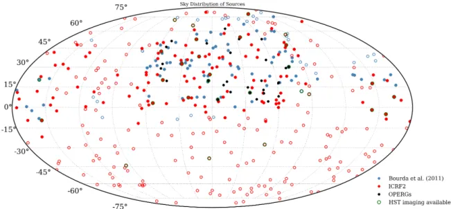
2.2. Sky distribution of the ICRF2+ and of the OPERGs sources . . . 17

3.1. Examples of Sérsic profiles . . . 22

4.1. Scheme of the Radon transform . . . 28

4.2. Schematic representation of image rotation . . . 29

4.3. Image reconstruction from multiple 1D profiles . . . 29

4.4. 2D galaxy model from GALFIT . . . 32

4.5. Re-sampling of the galaxy to accommodate the rectangular shape of Gaia’s pixel 33 4.6. Radon transform of the galaxy model and corresponding observed angle selection 33 4.7. Simulated Gaia image for the model galaxy . . . 34

4.8. Example of poissonian re-sampling of an image . . . 35

5.1. Flux ratios of the sources: wings vs. central region . . . 38

5.2. Magnitude results from GALFIT and class number count normalized histogram as a function of redshift . . . 39

5.3. Distribution of residual light after model subtraction . . . 41

5.4. Residuals distribution per morphological class . . . 41

5.5. GALFIT results for ICRF2+ sources with PSF profiles . . . 43

5.6. Surface brightness profiles and isophotal contours for the sources of figure 5.5. . . 44

5.7. GALFIT results for ICRF2+ sources with Sérsic profiles. . . 45

5.8. Surface brightness profiles and isophotal contours for the sources of figure 5.7.. . 46

5.9. GALFIT results for ICRF2+ sources with PSF+Sérsic profiles. . . 47

5.10. Surface brightness profiles and isophotal contours for the sources of figure 5.9.. . 48

5.11. Structural parameters results from GALFIT. . . 49

5.12. Comparison of surface brightness profiles between SDSS DR9 and Stripe 82 data 50 5.13. Example of HST modelling of an ICFR2 source . . . 51

5.14. Distribution of Sérsic indexes of the optically passive elliptical radio galaxies . . . 52

(18)

5.16. Surface brightness profiles and isophotal contours for the galaxy of figure 5.15. . . 53

5.17. GALFIT results for an OPERG with two components . . . 53

5.18. Surface brightness profiles and isophotal contours for the galaxy of figure 5.17. . . 54

5.19. Central regions of perturbed galaxies from HST images. . . 55

5.20. GALFIT results for galaxy SDSS J170045.23+300812.8 . . . 56

5.21. HST surface brightness profiles for galaxy SDSS J170045.23+300812.8 . . . 56

5.22. Simulation results for three simulation configurations: Ib. . . 58

5.23. Simulation results for three simulation configurations: rb. . . 59

5.24. Simulation results for three simulation configurations: Id. . . 60

5.25. Simulation results for three simulation configurations: rd. . . 61

5.26. Simulation results for three simulation configurations : b/a. . . 62

5.27. Mean errors as a function of simulated column . . . 63

5.28. Comparison between input and output values for the nine galaxies simulated with GIBIS . . . 66

6.1. Comparison between input and output values for the 28 OPERGs simulated with my code . . . 71

(19)

LIST OF TABLES

1.1. Window sizes of Gaia . . . 12

5.1. Number summary of ICRF2+ sources. . . 39

5.2. Table with the defined intervals from which the galaxy parameters are taken. . . 55

5.3. Median errors as a function of simulated column . . . 63

5.4. Table with the input parameters required by GIBIS . . . 65

7.1. ICRF2+ sources with HST imaging available . . . 77

7.2. Summary table with information for the 28 OPERGs . . . 78

7.3. Table with morphological information for ICRF2+ sources . . . 79

7.4. Table with morphological information for OPERGs . . . 86

(20)

(21)

PREFACE

From our home on the Earth, we look out into the distances are strive to imag-ine the sort of world into which we are born. (...) But with increasing distance our knowledge fades, and fades rapidly, until at the last dim horizon we search among ghostly errors of observations for landmarks that are scarcely more sub-stantial. The search will continue. The urge is older than history. It is not satisfied and it will not be suppressed.

- Edwin Hubble, The Law of Red Shifts, 1953

The emergence of the study of celestial bodies outside of our own galaxy can be pinpointed to the middle of the 18th_{. On that epoch, Thomas Wright, hypothesized about the possibility of}

some of the nebulae that were observed in the skies might be actually outside of our own Milky Way. Some years past that time, Immanuel Kant came up with the “island universes” terminol-ogy to refer to these possibly distant objects. Almost a century later, François Arago revived the hypothesis of nebulae outside our own (Arago, 1854) thus creating momentum for the idea to take roots in the scientific community. However, some of those nebulae, first compiled by Messier (1784) with a complete diﬀerent purpose, were actually part of the Milky Way (such as planetary nebulae or globular clusters). A compilation of new observations had to be made to spread some light on this controversial topic. William Herschel and Lord Rosse both contributed greatly by observing several thousand sources and by being able to distinguish point sources within the extended nebulae giving support to the idea of the existence of distant extragalactic sources. Slipher (1913) observed the spectra of some of those nebulae and found that some of them had their lines deviated from their laboratory position towards redder wavelengths leading to the measurement of their recessive motion relative to the Milky Way at a greater speed than that needed to escape from our galaxy.

This problem was finally solved in the 1920s. In the beginning of that decade, Curtis (1920) presented several evidences on why the Andromeda “nebula” M31 is a galaxy itself, like ours. Öpik (1922) estimated its distance from us that puts it at 450 kilo-parsec away. Still around two times smaller than its current measurements, but far enough to be exterior to the Milky Way. Taking advantage of the large aperture of the Mount Wilson Telescope, Edwin Hubble observed a number of Cepheid stars (whose characteristic variable brightness allows one to compute their absolute magnitude) and, using the distance modulus, confirmed the large distance of these ob-jects while still underestimating their actual value by a factor of ⇠3 due to calibration oﬀsets. Based on the images of the galaxies he also devised a scheme for classifying them according to their overall shape - the Hubble (1926) sequence - and stated that the Universe is currently expanding (Hubble, 1929), the foundations of modern cosmology.

(22)

As more and more images and spectra were obtained, new mysteries started to puzzle as-tronomers. Seyfert (1943) uncovered the presence of strong emission lines superimposed on a regular-like spectrum arising from the centre of a sample of six galaxies. Some were narrow, and some were broader but both were strong enough to compel a search for this newly found evidences. Woltjer (1959) denoted that the required central mass (< 100 pc) to support such an intense light emission should be of about 108 _{M . Thus, the first idea proposed by Hoyle &}

Fowler (1963) was that a very massive star-like object resided in the centre of those galaxies which would produce the emission lines from the accretion of surrounding gas through a rotating disc. A year later, the hypothesis of the core of the active galactic nuclei (AGN) was actually a black hole and not a super massive star came to existence (Salpeter, 1964; Zel’dovich & Novikov, 1964). This notion of a super massive central black hole which led to an active galactic nuclei and is also present in the centre of our own galaxy (Lynden-Bell & Rees, 1971) was a strong theory that explained several facets of the observed facts. It explains the existence of large amounts of energy emitted through the accretion of matter, the subsequent release of gravitational energy and also the limited size of the regions responsible for that emission with its subjacent short time scales of variability detected in AGNs. A new field arose to study all the related physical phenomena that are responsible for the observed emission in a very broad range of the electromagnetic spectrum and all the processes involved in the formation, evolution and distribution of this kind of objects in the Universe.

After years of dedicated research, we are now closer to understanding these fascinating objects with impressive energy liberation from the central super massive black holes which are intriguing objects on their own. Apart from their core body, the accretion disc, the warm dust torus and all the surrounding gas take part in the global picture of what an AGN is. These, in turn, aﬀect the formation and subsequent evolution of the galaxies that we observe leaving their imprint in the structure of the Universe at large scales. But, as it is always the case in science, we are still far from fully understanding this particular “specimens” of our Universe and more hours of observations and years of research are required to acquire a little bit more of comprehension of what is around us.

In this dissertation, several AGN will be studied in detail with the aim of understanding their morphology and its impact in future studies with the forthcoming Gaia mission. The prime interest lies in quantifying the structure of the underlying host galaxies that harbour AGN in their centre. The main observational tool for this research is the photometry obtained in the optical domain by the Sloan Digital Sky Survey Data Release 9 and, when possible, the archive of the Hubble Space Telescope.

(23)

CHAPTER

1

INTRODUCTION

“Some people believe that without history, our lives amount to nothing. At some point, we all have to choose. Do we fall back on what we know? Or, do we step forward, to something new? It is hard not to be haunted by our past. Our history is what shapes us, what guides us. Our history resurfaces. Time, after time, after time. So we have to remember. Sometimes, the most important history, is the history we are making today.”

- Time After Time; Grey’s Anatomy

Contents

1.1. Active Galactic Nuclei . . . 2 1.1.1. AGN Types . . . 2 1.1.2. The Physical Picture of AGN . . . 3 1.1.3. The Spectral Energy Distribution of AGN . . . 4 1.1.4. AGN Galaxy Hosts . . . 6 1.2. Optically Passive Elliptical Radio Galaxies . . . 6 1.3. The International Celestial Reference Frame . . . 7 1.4. Astrometry: from Hipparchus to Gaia Era . . . 8 1.4.1. Gaia Galaxy-Mapping Satellite . . . 9

This dissertation investigates a sample of extragalactic objects in the optical band, in the frame-work of the Gaia (ESA) mission. The specific samples under analysis in the context of this project are:

• a set of the International Celestial Reference Frame (ICRF) sources that will enable the connection between the ICRF and the Gaia Celestial Reference Frame, GCRF. These are mainly blazars that show a very compact optical morphology, mostly being emission related with the powerful AGN. The sample comprises the ICRF2 defining sources together with a proposed extension by Bourda et al. (2010);

• a set of optically passive AGNs living in elliptical galaxies that show little or no extra activity in the optical regime, i.e. a kind of counterpart of the previous set of objects. The global aim of this dissertation is to model the 2-dimensional surface brightness profiles of the objects using the most common software for this kind of analysis - GALFIT (Peng et al., 2002, 2010) - in order to characterize any detectable host galaxy for the case of the compact objects and to assess the Gaia detectability of the AGN galaxy hosts through the Gaia Instrument and Basic Image Simulator (GIBIS, Babusiaux 2005; Babusiaux et al. 2011) based on the elliptical

(24)

galaxies sample. The following chapters are arranged as follows: in this first chapter I present an introduction to the field of AGN research. It is meant to contextualize the reader on this topic and to highlight some of the aspects of this field that will be useful for the comprehension of this dissertation. It also serves to delineate the motivation that supports this work. Thorough analysis and descriptions of this class of objects may be found in the books by Robson (1996), Peterson (1997), Osterbrock & Ferland (2006), Krolik (1999) and Beckmann & Shrader (2012). In the discussion here presented, I will emphasize the Gaia applications to the extragalactic field, which may also be found with greater detail in Andrei et al. (2012a), Mignard (2012), Krone-Martins et al. (2013) and de Souza et al. (2014).

In Chapter 2, I describe with some degree of detail the Sloan Digital Sky Survey (York et al., 2000; Ahn et al., 2012), which is the survey from which the images to be analysed are retrieved thus being the basis of the entire project. Chapter 3 includes a brief discussion on how GALFIT works and how the required files were prepared and all the data were collected, in particular by using SExtractor (Bertin & Arnouts, 1996) so that I could successfully conclude the 2D analysis. Post-processing tasks are also described in detail, including the creation of the 1D surface brightness profiles using the capabilities of IRAF (Tody, 1986, 1993). In Chapter 4, I introduce the reader to the description of the algorithm for the construction of images of galaxies as seen by Gaia, which includes the definition of the Radon transform, to be used in simulations to assess the eﬃciency in recovering structural parameters of galaxies. All the results obtained from the previous chapters are then presented and analysed further in Chapter 5 so that one can extract the maximum amount of information from the available data. I discuss all the results in light of the current knowledge and summarize all the main outcomes from my work in Chapter 6. Finally, in Chapter 7 I draw attention to the main conclusions that can be taken from this project and suggest future following up studies.

1.1. ACTIVE GALACTIC NUCLEI

The name “active galactic nucleus” (AGN) was coined due to the observational fact that galaxies often possess an unusually high concentration of energy liberation in their central regions. This energy is not explained by the normal energy output that one would expect from stars. In addition to that, they also emit in a broad range of the electromagnetic spectrum: from radio to

-rays. In the next subsections I will detail briefly the characteristics of this kind of objects. 1.1.1. AGN TYPES

The first evidence for the existence of an AGN was the detection of strong emission lines in the spectrum of galaxies that exceeded by far any previous class of discovered objects. But as more and more spectra were compiled, astronomers started to note that not all active galaxies possessed the same features. The emergence of such cases lead to the establishment of several types of AGN according to their main properties.

Seyfert galaxies, named after Seyfert (1943) who presented a small sample in an article about this class of objects. These are regular spiral galaxies with strong nuclear emission. Khachikian & Weedman (1974) divided this further class into two subclasses according to the broadening of its spectral lines. Seyfert type 2 galaxies have narrower ( . 1000 km s 1_{) forbidden and permitted}

emission lines than those that appear in Seyfert type 1 galaxies ( ⇠ 1000 5000 km s 1_{). It}

is observed that there are more Seyfert type 2 galaxies than Seyfert type 1 and that all Seyfert galaxies comprise around 3% to 5% of all galaxies (Maiolino & Rieke, 1995; Maia et al., 2003). Radio galaxies, as discovered by Brown & Hazard (1959) and Edge et al. (1959), are AGNs that emit strongly at radio wavelengths. The radio emission may not be concentrated only in

(25)

the central region of the galaxy, but extends to great distances (up to hundreds of kpc and even reaching Mpc scales) via jets emanating from the nucleus. Usually in pairs, the jets consist of a collimated beam of relativistic particles moving through a magnetic field leading to synchrotron radiation emission. Whenever the jet material interacts with the intergalactic medium, it usually forms a lobe.

By looking at the optical spectra of these radio sources they might be also classified as Broad Line Radio Galaxies (BLRGs) and Narrow Line Radio Galaxies (NLRGs) in the same manner as one distinguishes the two diﬀerent kinds of Seyferts. Another distinction based on their radio morphology has also been proposed by Fanaroﬀ & Riley (1974): FR-I objects which have their lobes separated by less than half of the host galaxy and FR-II objects for which the separation is larger. They are commonly associated with weak and strong radio power, respec-tively.

As a powerful example of radio galaxies there are quasars (“quasi stellar radio sources”), the most energetic objects in the Universe which possess a star-like appearance in the optical domain. They first puzzled astronomers with their odd-looking spectral lines which were recognized by Schmidt (1963) as a redshifted UV spectrum that placed these objects at great distances from us. Similar to quasars there are the “quasi-stellar objects” (QSOs) which are radio-quiet, but high-luminosity AGN some with a star-like appearance in their optical images. These two types of objects are often simply referred as quasars. The star-like appearance is due to the high-luminosity of the central region combined with the great distance at which these objects are. Thus, the underlying host galaxy is in generally hard to detect in the images.

There is the blazar class (e.g. Urry & Padovani, 1995) that stands for BL Lacertae (BL Lac, named after its first detected object which was thought to be a variable star (Schmitt, 1968)); Optically Violent Variable sources (OVVs, McGimsey et al. 1975) and Flat Spectrum Radio Quasars (FSRQ, Andrew & Kraus 1970). They possess the common property of having highly variable luminosity on time scales as short as some hours, some emitting highly polarized pho-tons.

1.1.2. THE PHYSICAL PICTURE OF AGN

The myriad of classes presented in the previous subsection has one thing in common: a big amount of energy is released from a very small volume in space. In the brightest quasars, their luminosity can reach values of 1041 _{W, which is 10}15 _{brighter than the energy output from the}

Sun. The current paradigm states that such among of energy must come from the release of gravitational energy from mass accretion by a super massive and compact object, like a super massive black hole based on ideas proposed by Salpeter (1964), Zel’dovich & Novikov (1964) and Lynden-Bell (1969).

The idea behind the unification of the various classes of AGN is based on the fact that all the observed diﬀerences might be explained by a small set of parameters (Antonucci, 1993; Urry & Padovani, 1995), namely the luminosity, the relative orientation of the AGN with respect to the line of sight and the presence (or not) of radio jets.

By combining the physical model with the observed types of AGN, one is able to dissect the AGN into its various components, each of which is responsible for diﬀerent observed features. The main components are summarized below:

• A super massive black hole with masses ranging from 106 _{up to 10}10 _{M which resides}

(26)

Figure 1.1. The current picture of the unified model of AGNs. Considering the line of sight of the observer with respect to the AGN orientation, the observer sees different classes of AGNs. For radio-quiet objects the orientation effect leads to the observed Seyfert classes. For radio-loud objects there is the combination of morphology+orientation effects to account for the different observed classes. Graphic courtesy of Marie-Luise Menzel for the book Beckmann & Shrader (2012, Chapter 4).

.

• An accretion disc of size ⇠ 0.1 pc composed by optically thick and hot plasma (⇠ 104 ₁₀6

K) which is the main driver of the energy release by the AGN and surrounds the central black hole;

• A broad line region, with sub-parsec scales, which accommodates clouds of high density gas that orbit the black hole at extremely high velocities. The gas is excited by the radiation that comes from the accretion disc and emits permitted and broad emission lines of ionized elements;

• This central part of the AGN is enclosed by a dusty molecular torus with several parsecs in size. Its inner boundary is defined by the sublimation temperature of the dust, which is around 1500 K;

• At even larger distances, from 10 to 1000 parsecs, it is located the narrow line region which is composed of lower density gas clouds that are mostly located upwards and down-wards the torus. The photons coming from the radiation field of the central region of the AGN ionize the atoms of the clouds producing permitted and forbidden lines with narrow widths;

• Finally, collimated jets originating from the AGN core and perpendicularly to the accretion disc extend out to several kpc and up to Mpc scales. The interaction of the jets with the surrounding medium leads to the production of lobes.

Since different regions are harbouring different physical phenomena that produce photons in different ranges of energies, it is expected that looking through different directions yield different observations of the same object. As seen from figure 1.1., the orientation of the line of sight with respect to the AGN modifies its observational properties thus changing the object classification.

1.1.3. THE SPECTRAL ENERGY DISTRIBUTION OF AGN

As stated before, the emission of the AGN covers the entire electromagnetic spectrum and its typical energy distribution along the spectral range is summarized in figure 1.2.. Below I will

(27)

describe the physical processes underlying the continuum emission in each wavelength range fo-cusing on the radio and optical regimes.

Figure 1.2. Schematic distribution of the spectral energy of a typical radio quiet and radio loud AGN source. From Carroll & Ostlie (2007, chapter 28).

Starting with the radio regime, the main physical process among radio-loud objects is synchrotron radiation. This radiation is characterized by photons emitted from accelerating relativistic elec-trons moving along spiral paths around the lines of the magnetic field. In terms of morphology there is the extended emission associated with the jets and the lobes (the regions of interaction of the jet material with the surrounding environment) of the AGN. There is also the compact component, often named core emission, which is thought to be related with the region where the jet forms and where it is believed to be optically thin. It is the combination of the multiple syn-chrotron emission of electrons at diﬀerent speeds that produces the observed shape of the SED in the radio regimes. It consists of a simple power law, F⌫ / ⌫ ↵, where ↵ is the spectral index

and varies according to the region one is considering. By comparing the flux of the continuum from the radio to the optical one derives the useful quantity (Beckmann & Shrader, 2012)

R⇤= fradio fB

, (1.1)

which is used to define the separation between radio quiet (R⇤ _{< 10}_{) and radio loud (R}⇤ _{> 10}₎

galaxies. It is found that nearly all AGN (⇠ 90%) are radio quiet.

In the infra-red regime there can be thermal and non-thermal origins for this emission. For radio-loud objects, namely blazars, the synchrotron radiation may dominate in this regime, and in other AGNs dominates the dust emission.

One striking feature of the optical regime is the big blue bump in the continuum emission thought to be of thermal origin and which extends into the ultraviolet range. This bump is thought to be the black body radiation emanating from the hot gas in the accretion disc around the central black hole. There is another small blue bump, often unnoticed, that is considered to be to a blended emission of iron lines and the Balmer continuum. Jets might also contribute to the optical emission in certain configurations. Apart from the continuum features the presence of strong narrow or broad emission lines also marks the optical spectrum of AGNs.

(28)

As an extension to the optical regime, the UV range of the AGN SED is dominated by the thermal emission, strong lines (emission and absorption) related to the central hot gas of the accretion disc.

The X-ray spectrum reflects two diﬀerent physical regimes. The first, at lower energies (. 1 keV), is generated by inverse Compton scattering of photons emitted from the thermal emission of the accretion disc by the electrons of the hot gas that surrounds the central region of the AGN. The second, referred as the “reflection hump”, between 10 and 30 keV (George & Fabian, 1991) which comprises photo-absorption, iron fluorescence and Compton scattering of relatively cold gas very near the central black hole.

1.1.4. AGN GALAXY HOSTS

All AGNs reside in galaxies. Even the most elusive and compact hosts have been revealed in deeper studies of a number of objects. Nevertheless, in the case of the quasars, is really hard to detect the hosts with current instruments, either because they are too compact, too faint or simply because the contrast between the central powerful AGN and the extended emission from the galaxy is huge (Bahcall et al., 1997). And, since they reside inside galaxies there is a lot of discussion around the influence of the host galaxy in the AGN and vice versa. Comprehensive reviews on this topic may be found, for example, in Veilleux (2008), Cattaneo et al. (2009), Fabian (2010) and Kormendy & Ho (2013).

The open topics under scrutiny in this particular field are aiming to uncover any relations that might exist between the properties of the AGN and of its host galaxy. It appears that there is a relation between the Hubble type of the galaxy and the amount of matter that is accreted by the black hole (e.g. Ledlow & Owen, 1995; Falomo et al., 2014). And, there are some relations that have been proposed that relate the host mass, or the mass of the bulge of the host with the mass of the black hole (e.g. Gebhardt et al., 2000; Häring & Rix, 2004). The tendency found is that more massive black holes are encountered in the heart of the most massive galaxies, which in turn tend to be ellipticals rather than spirals. There is also an attempted connection between the star formation of hosts and the power of the AGN which in turn relates to the feedback (the impact of the AGN on the star formation of the host galaxy) problem, which is not yet fully understood (Santini et al., 2012, and references therein).

Other related subjects concern the growth of the mass of the central black hole (see Kormendy & Ho, 2013, for a detailed discussion). Whether it happens via mergers of smaller ones or instead via a continuous secular growth by mass accretion of matter of the host galaxy it is still open to debate. Both seem to play their part, but far too much is still to be found in future research. 1.2. OPTICALLY PASSIVE ELLIPTICAL RADIO GALAXIES

Elliptical galaxies tend to be passive in the sense that they produced little or no amount of new stars in their recent past (1-2 Gyr, e.g. Sparke & Gallagher, 2007, chapter 6). Therefore, their bulk of emission comes from older stars, and less massive stars which have not yet succumbed to their fate. These kinds of stars are cooler that the young and massive stars thus presenting redder colours.

Radio-loud AGNs are mostly found in elliptical galaxies (Taylor et al., 1996). Among the low luminosity radio-loud objects there are some that show little evidence for extra activity in the optical regime, even though possessing strong emission at the radio regime (e.g. Antón et al., 2004; Antón & Browne, 2005). These particular type of AGN tend to live in red elliptical galaxies

(29)

and have therefore been named as Optically Passive Elliptical Radio Galaxies (OPERGs). The fact that in the optical domain the nuclear emission is diluted in the stellar component makes them good targets for the analysis of their hosts.

In what regards their SED some of these objects have similar properties to BL Lacs in some re-gions of the electromagnetic spectrum when not taking into account the optical and near-infrared emission, which are dominated by stellar emission. They present a smooth transition from radio to sub-millimetre regimes (Antón et al., 2004) and sometimes a core-jet radio morphology (Antón et al., 2004; Bondi et al., 2004). In many aspects they are indistinguishable from BL Lac objects in the longest wavelength regimes, and has been proposed that OPERGs are blazars with a low frequencies peak in the non-thermal component or intrinsically weak AGN (Bondi et al., 2004). 1.3. THE INTERNATIONAL CELESTIAL REFERENCE FRAME

Ideally, a celestial reference frame should be established by the same objects observed at all wavelengths (Walter & Sovers, 2000). This would make easier to establish cross-identifications between sources detected from the radio to -rays wavelengths. In practice, such construction is not easy to achieve since there are not in the Universe many objects that fulfil all the re-quirements to constitute a good reference source: being bright, compact and without proper motion (Taris et al., 2013). Being powerful, emitting in several wavebands and apparently very compact, quasars are among the best candidates to provide a link between reference frames in the optical and radio domains. The fact that they are at big distances from us also minimizes the problems of proper motions that would imply a limitation in the definition of the reference frame. However, at optical wavelengths, they might not be bright enough to be detected or even if brighter enough they might not possess compact morphology in their radio emission (Orosz & Frey, 2013; Taris et al., 2013).

Nowadays, the best precision that astronomers can achieve in the measurement of absolute po-sitions happens at radio frequencies (Charlot & Bourda, 2012) and the International Celestial Reference Frame (ICRF) is based on observations of distant sources (namely blazars) using Very-Long-Baseline Interferometry (VLBI) radio telescopes. The first version of the ICRF (Ma et al., 1997; Ma & Feissel, 1998) was defined by the positions of 212 compact radio sources. However, the compilation of additional data and new observations of additional sources with time lead to the 2nd _{realization of the ICRF, which is now composed of 295 defining sources}1 _{and is referred}

as ICRF2 (Fey et al., 2004, 2009).

Objects with core radio morphology, absent proper motions, apparent optical point-like nature are assumed to have a high degree of accuracy and stability of their coordinates and for that reason they can help on the alignment between the ICRF andjm reference frames of similar ac-curacy like the Gaia mission (Bourda et al., 2008), (Bourda et al., 2010), (Bourda et al., 2011), (Mignard, 2012), (Charlot & Bourda, 2012), (Andrei et al., 2012a), (Andrei et al., 2012b) and (Taris et al., 2013). The high astrometric accuracy of Gaia will make possible to establish a reference frame in the optical domain.

While it is not yet possible to get the astrometric measurements of Gaia, we can study the suitability of the candidates for the alignment between the two reference frames based on existing and public data such as the Sloan Digital Sky Survey (SDSS) which is the largest sky survey that we can access. There are several works devoted to the issues related with oﬀsets between the radio and optical centroids (e.g. Orosz & Frey, 2013, and references therein). Here, we

1_{A defining source is a source which has high-astrometric-quality over the entire period of observations available}

(30)

concentrate in the impact that the AGN host galaxy may have for the astrometric accuracy at the optical band. In that sense, a census of the available images of the already radio accurate reference sources to inspect their morphological structure is necessary to verify the detectability of the host galaxies.

1.4. ASTROMETRY: FROM HIPPARCHUS TO GAIA ERA

Astrometry is as old as men. It refers to the study of the geometrical relations between objects in the sky and their motions and it has been fundamental in the progress of astronomy until the 19th

century. Nowadays it remains a basic element fundamental for any astronomical related research. The first geometrical relation that one often uses is the parallax. This eﬀect occurs as a natural consequence of the motion of the Earth revolving around the Sun. The idea is to compare the position of a nearby object observed with a separation of six months which is roughly the time that Earth takes to move between opposite positions in relation to the Sun. As seen in figure 1.3., this will produce a separation between the two apparent positions of a nearby source. The parallax is then defined as half the angular separation of a source’s position observed at opposite Earth locations with respect to the Sun. By using the measured parallax it is straightforward to use the trigonometric relations to compute the distance from the Earth to the source as

sin(⇡) = 1AU

d , which for ⇡⇡ 0 becomes ⇡ ⇡ 1AU

d . (1.2) This measurement is even used to define a commonly used unit in astronomy: the parsec, which is, by definition, the distance that a source has to be to produce an observed parallax of one sec-ond of arc. Despite simple, this technique is limited by the resolving power of current telescopes as much of the angles that one has to measure are extremely small.

1A U Source D ist an t Ba ck gr ou nd ⇡ ⇡

Figure 1.3. Parallax definition from the opposite positions of the Earth (blue circle) relative to the Sun (yellow circle) and the apparent position of the source (grey rectangle) superposed in the background (light grey rectangles). The angle ⇡ is the parallax of the source.

Apart from measuring distances, astrometry also serves to determine the motion of objects in the space relative to each other. This motion can be further separated into two components, the radial velocity, which is measured along the line of sight and the proper motion, which is the transverse movement across the sky. The first is easily measured from observing the Doppler shifts in the spectral lines of the source by contrast the second is much more diﬃcult to determine as it requires careful observations of the object with respect to many others over an extended period of time, usually years.

Obtaining distance and motions of objects is crucial to our comprehension of how the Uni-verse works. Using the distance we can determine the luminosity and size of the object one is

(31)

considering, using the motions we can infer its trajectory in both time directions: future and past. It was in the dawn of mankind, many centuries ago that men started to look to the heavens. They realized that objects moved in a particular and regular way across the sky thus rendering it useful to determine directions and time on the Earth surface. The urge to plan their life hastened the need for precision astrometry so that one could, for instance, maximize the output from a plantation by planting and harvesting at the right moments.

In ancient Greece, around 100 B.C., with no help from any instrument, Hipparchus compiled the first catalogue of sources with specified brightness and positions as accurate as one degree, which is roughly two times the diameter of the full moon. This first catalogue marked the birth of astrometry. After that, it has seen little progress until the 16th _{century when Tycho Brahe}

revolutionized the field, establishing a new accuracy limit in ⇠1 minute of arc (60 times better that Hipparchus). He designed, built and then calibrated a variety of measuring instruments like the sextant or the mural quadrant, which greatly changed the way observations were done. It was Tycho’s measurements that allowed Kepler to later establish that the planets moved in elliptical orbits around the Sun.

With the invention of the telescope in the early years of the 17th _{century new doors opened to}

achieve better precision and measure even smaller angles. Combined with a mechanical support that allowed to precisely move the telescope (the filar micrometer invented later in that century) it allowed scientists to break the barrier of one minute of arc imposed by the limitation of our eyes. The improvement of other techniques such as the possibility to engrave observations al-lowed for the detection of the stellar aberration in 1725 and the detection of the motion of sources in the sky by Edmund Halley. This evolution of the technology leads to the first measurements of the parallax in the 1830s laying grounds to the idea that those bright sources that we observed were actually at finite distance from us and had mankind rethink our place in the Universe. The limits were pushed further down to ⇠ 0.1 arc seconds, which is the limit of Earth observations imposed by atmospheric eﬀects.

It was only in the end of the last century that the first space based telescope dedicated to astrometry, Hipparcos, was launched by ESA in 1989, and allowed an improvement of 100 times more precision than previous studies and compiled a list of ⇠120000 objects with precisions of one milliarcsecond. Following this success, ESA has planned a new mission, Gaia, to increase even further our measurements in precision (see figure 1.4.) and in number of observed sources. This mission is described with greater detail in the following subsection.

1.4.1. GAIA GALAXY-MAPPING SATELLITE

Gaia, whose name originated as an acronym of Global Astrometric Interferometer for Astro-physics (despite not having an interferometer in its final design, the name has been maintained), is a successor to ESA’s Hipparcos mission and it was launched in December 2013. It is stationed at the L2 Lagrangian point of the Sun-Earth system, 1.5 million km from the Earth in the direc-tion away from the Sun. As an ESA space-based mission, planned during the 90s, it has as its main goal performing astrometric measures of galactic sources in order that we can reconstruct 3-dimensional maps of our vicinity with an unprecedented precision of ⇠ 7 µas for sources up to G = 122 and ⇠ 25 µas for fainter objects up to G = 15 and a maximum precision of 30 mas for the faintest objects detected with G ⇡ 20. It will provide a major improvement on parallax mea-sured distances of roughly ten million stars in a 2.5 kpc radius with 1% precision. In addition, Gaia is expected to discover large numbers of other celestial bodies such as comets, asteroids,

(32)

Figure 1.4. The evolution of the accuracy in astrometry measurements throughout time. Adapted from The Little Book of Gaia: History of Astrometry: http://www.esa.int/Education/ Little_Books_of_Gaia.

exoplanets, brown dwarfs, variable stars and supernovae. Nonetheless, despite its main goal of measuring distances within the Milky Way, its sensitivity will allow the detection and observation of extragalactic objects of extended nature and point-like sources such as quasi-stellar objects (QSOs). This measurements will then allow a direct establishment of an extragalactic celestial reference frame (Gaia Celestial Reference Frame - GCRF) derived in the optical range.

The Gaia strategy to obtain precise astrometric measurements consists on measuring angles be-tween distinct objects, which is made possible by multiple observations of the same targets in diﬀerent orientations (diﬀerent great circles passing through a given object). To complete its objective, Gaia is composed of two identical telescopes with rectangular mirrors which observe almost opposite regions of the sky (106.5 apart) with a continuous precession movement allow-ing for a complete census of the celestial sphere. The satellite completes a great circle every six hours and has a 63-days cycle of the precession movement. Each of the telescopes has a mosaic of 106 CCDs of 4500 ⇥ 1966 pixel each. Each pixel has the particularity of being rectangular covering a region in the sky of 59⇥177 mas (see figure 1.5.).

This mosaic of CCDs has diﬀerent sets of columns each corresponding to a specific science ob-jective. Those columns are highlighted in diﬀerent colours in figure 1.5.. The first two columns are named as Sky-Mappers (SM) and each of them is responsible for the detection of sources from light coming from a specific telescope, i.e., the first column serves to detect sources coming from one telescope and the second column to detect sources observed from the other telescope. The other CCD columns receive the light coming from both telescopes. As Gaia is constantly moving across the sky, the sources detected in the first two columns will be followed across the nine columns that compose the Astrometric Field (AF). The first eight columns have seven rows of CCDs and the last one has only six rows. This configuration will allow the instrument to follow and record the position of each source as they move from one column to another. After going through the Astrometric Field, the light of each source passes through a blue photometer,

(33)

Figure 1.5. Scheme of the CCD mosaic on board of Gaia. Credit: Alexander Short - ESA. measuring light from 3300 to 6800 Å, and then by a red photometer measuring the light from 6400 to 10000 Å. This is done in order to obtain magnitudes in diﬀerent regions of the optical spectrum which will be used to characterize some physical properties of the observed objects. The final set of CCDs is part of the Radial Velocity Spectrometer instrument which will be used to measure Doppler shifts in the Ca II triplet lines by observing in the narrow band of 8470 to 8740 Å. These columns only examine the sources of first four rows of the Astrometric Field. Such measurements will allow for the measurement of the velocity of the observed stars along the line of sight.

Due to the huge amount of pixel information stored in theses mosaics, the transmission of the full observed data to Earth stations is technically impossible. In order to circumvent this issue, there is an on-board processing unit, which is responsible for the selection of the data to be transmitted. To do so, if a source is detected in the SM columns the movement of the source is followed in the AF columns by assigning a subset of pixels to the object to be stored in memory. Then, according to the source magnitude and its position on the CCD mosaic, the observed values are binned into the final data values which will be then transmitted to Earth. The window sizes as a function of CCD columns and source magnitude are displayed in table 1.1.. In this way, the data that reaches a ground station and will be subsequently analysed corresponds to a window around object composed of samples each of which is a sum along the binning directions of the observed window. For example, a G = 15 magnitude object will be transmitted from AF2 as a set of 18 values where each value corresponds to the sum of the 12 pixel along the perpendicular direction of the CCD movement (see figure 1.6. for a schematic representation). For most cases (G > 13) in the Astrometric Fields only 1-dimensional data will be transmitted to Earth. Thus, in order to be able to analyse the extended emission of extragalactic sources it

(34)

will be necessary to reconstruct the 2D signal from the set of available data via a well-known mathematical process which uses the Radon transform of the signal and is, for instance, widely used in Computerized Tomography scans.

CCD column Gmag Window Size Binning factor Window size (read, in pixel) (in sample, transmitted) SM G<13 80⇥12 2⇥2 40⇥6 G>13 80⇥12 4⇥4 20⇥3 G<13 18⇥12 1⇥2 18⇥6 AF 1 13<G<16 12⇥12 1⇥12 12⇥1 G>16 6⇥12 1⇥12 6⇥1 G>16 18⇥12 1⇥1 18⇥12 AF 2,5,8 13<G<16 18⇥12 1⇥12 18⇥1 G>16 12⇥12 1⇥12 12⇥1 G>16 18⇥12 1⇥1 18⇥12 AF 3,4,6,7,9 13<G<16 12⇥12 1⇥12 12⇥1 G>16 6⇥12 1⇥12 6⇥1

Table 1.1. Window sizes of Gaia imaging processing data as a function of CCD column and source G band magnitude. Translated from Krone-Martins (2011, chapter 2).

Figure 1.6. Window over position of diﬀerent CCD columns on top of simulated images of idealized galaxies with Sérsic profiles. The yellow lines represent the samples to be transmitted to Earth while the red lines represent the pixel limits of the CCD. For the AF columns, the image is zoomed to better understand the window configuration.

(35)

CHAPTER

2

DATA & SAMPLE

“[T]he key to making progress is to recognize how to take that very first step. Then you start your journey. You hope for the best and you stick with it, day in and day out. Even if you are tired, even if you want to walk away. You do not.”

- Man On The Moon; Grey’s Anatomy

Contents

2.1. Data from Sloan Digital Sky Survey . . . 13 2.1.1. The Survey . . . 14 2.1.2. Astrometric/Photometric Quality . . . 15 2.2. Sample Description . . . 16 2.2.1. ICRF2+ . . . 16 2.2.2. OPERGs. . . 16

As said in the previous Chapter, two sets of objects are under study in this dissertation: the ICRF objects which are believed to be mainly point-like sources in the optical regime and a sample of nearby optically passive elliptical radio galaxies. Given the objective of investigating the presence of any extended component that might perturb the astrometric evaluation of the object’s position, it is important to refer the parent sample and describe the real sample under scrutiny. The mentioned samples are not the same due to SDSS limitations in terms of covered regions. Details on each of the defined samples and on the SDSS survey used to carried out this project are explained in detail in the sections that follow.

2.1. DATA FROM SLOAN DIGITAL SKY SURVEY

The Sloan Digital Sky Survey (SDSS, York et al. 2000) is one of the greatest survey projects of modern astronomy. Its huge eﬀorts are aimed to map around 25% of the sky and deter-mine the position and apparent magnitude of more than ten billion objects. It also comprises a spectroscopic follow up that serves to measure up to a million redshifts of local galaxies and distant bright quasars. With its fourteen years of operations, divided in three phases (SDSS-I, 2000-2005; SDSS-II, 2005-2008; SDSS-III, 2008-2014), it is the most extensive survey ever taken and its wealth of data allows scientists around the world to significantly advance in the under-standing of extragalactic astronomy and unravelling the steps that take place in the evolution of galaxies. In this section, I briefly describe the survey and I point out your attention for the SDSS astrometry and photometry quality to my study.

(36)

2.1.1. THE SURVEY

A dedicated 2.5-meter wide-angle optical telescope at Apache Point Observatory in New Mexico, United States of America, consists of an imaging survey of ⇡ steradians of the northern Galactic cap and also of a smaller area (⇠225 deg2_{) but much deeper images toward the southern Galactic}

cap. It takes images using a photometric system of five contiguous photometric bands - u, g, r, i and z - centred at 3540, 4770, 6230, 7630 and 9130 Å and with 95% completeness in typical seeing down to magnitudes of 22.0, 22.2, 21.3 and 20.5 mag, respectively. The filter system, described by Fukugita et al. (1996), covers the entire optical range from the near ultraviolet, where the limitation comes from the atmospheric absorption cut-oﬀ below ⇠ 3000 Å, to the redder limits imposed by the characteristics of the silicon that looses its sensitivity to photons with wavelengths larger than ⇠ 11000 Å. The transmission curves of the CCD in the SDSS’s five filters is shown in Figure 2.1. as a function of observed wavelength.

Figure 2.1. Transmission curves of the SDSS ugriz filter system plotted from the available tables at https://www.sdss3.org/instruments/camera.php#Filters.

To take the images, the telescope uses a drift scanning technique which consists of keeping the telescope pointed to a fixed region of in the sky and then takes advantage of the Earth’s rotation to map contiguous strips of the celestial sphere. As opposed to tracked telescopes, this technique allows for a more precise astrometric measurements over the wide field of view of the telescope as it is not aﬀected by errors in the tracking movement of those systems that surely aﬀect the position determination. However, this means that small distortions in the images are produced due to movement of the sources in the CCD focal plane. To minimize such distortions, the exposure times and reading times of the CCD must be kept to small values sacrificing thus the deepness of the survey.

The telescope is equipped with a 120-mega pixel camera composed of thirty CCD chips with 2048⇥2048 pixels which are arranged in five rows of six chips where each row has its own filter to simultaneously image the observed region in the five photometric bands. This camera can observe 1.5 square degrees of sky in a single observation, which is about eight times larger than the area of the full moon. It also has two spectrographs which are fed by optical fibers covering a circular region of 3" in diameter which are placed in the centre of the sources one wants to observe to measure the spectra (and thus redshifts/distances) of 1000 galaxies and quasars in a single snapshot (the original set-up of SDSS-I and SDSS-II allowed for a maximum of 640 targets

(37)

per pointing). It is interesting to note that the two key discoveries/technologies that are crucial to the functioning of SDSS, optical fibers and CCDs, were both awarded the 2009 Nobel Prize in Physics.

After obtaining the observations, a specific set of software pipelines processes the raw data obtained from the telescope to produce quality science images which are then ready for scientific exploitation. These pipelines also produce lists of observed sources and some of their related parameters, such as whether they seem point-like (like quasars or stars) or extended (as a galaxy usually is) and their apparent magnitude. The imaging data is processed with an automatic software pipeline called PHOTO (Lupton et al. 2002, 2001) and the morphological information derived from the images allows for robust star–galaxy separation to ⇠ 21.5 mag (Lupton et al. 2001; Yasuda et al. 2001).

2.1.2. ASTROMETRIC/PHOTOMETRIC QUALITY

To obtain reliable results from any image analysis done in astronomy, the quality of the main quantities must be assured. Those quantities are related with three techniques that are paramounts in any survey: photometry, astrometry and spectroscopy. Since the work carried out under this project is mainly related to image analysis, I will skip the discussion of the spectra quality as-sessment.

Astrometry is a useful technique that allows scientists to guide themselves through the sky. It is used to determine the true coordinates of sources, in any coordinate system that you may use or define (one ubiquitously used is the equatorial system where each position in the sky is defined by a set of two coordinates - right ascension and declination), departing from their physical position (usually in Cartesian coordinates - x and y) in the CCD. The idea that supports all astromet-ric solvers is simply to match a catalogue of reference sources, for which you now a priori the true sky coordinates, to a catalogue of detected sources in the images. In the case of SDSS, its astrometric calibration is described in great detail in Pier et al. (2003). I just want to highlight that the astrometric accuracy of the original SDSS set-up performs better than ⇠ 45 75 mas (depending on the reference source catalogue) which is below the minimum required accuracy of 180 mas so that the positioning of the optical fibers to obtain the spectra of sources could be executed successfully.

However, a number of issues prevented the accurate calibration of Data Releases - DR8 and DR7 - due to systematic oﬀsets found in some measurements. These were pinpointed and a new ameliorated pipeline was designed to incorporate solutions in the DR9 release that would remove the identified errors (Ahn et al., 2012). These corrections improved the accuracy of the measured positions and allowed for a better determination of the centroid oﬀsets of multi-wavelength com-parisons like those presented in Orosz & Frey (2013). Thus, it is fully justified that one uses the DR9 data to pursue the work.

As for the photometry, it is the technique related to the quantification of the amount of light that reaches the telescope from a given source, its brightness. Then, astronomers use a logarithmic scale to assign to each object an observed magnitude, which is simply defined as

m = 2.5 log₁₀(B) + C, (2.1) where B is the measured source brightness and C is a calibration constant. The calibration is done using reference sources for which we have known values of m. The flux of any object is measured normally in fixed size apertures centred on the source centroid. While this may work for stars and quasars, for galaxies, due to their extended shape and often irregular surface

(38)

brightness profiles, there are other methods to do so. One consists of fitting analytical models to the galaxy image and then minimizing the residuals to obtain the best fit parameters which include the object flux/magnitude. The other computes the flux within a locally computed aperture based on the Petrosian radius. This quantity, rp, is computed as the radius for which

the average surface brightness enclosed in an annulus (rp,in < r > rp,in) is equal to ⌘ times the

mean surface brightness measured inside the aperture with radius rp (Blanton et al., 2001).

⌘ = 2⇡ Rrp,out rp,in I(r)rdr ⇡r2_(1.252 _0.82₎ 2⇡Rrp 0 I(r)rdr ⇡r2

, with ⌘ = 0.2, rp,in= 0.8rp, rp,out= 1.25rp (2.2)

where I(r) is the azimuthally averaged surface brightness profile. The Petrosian flux is then defined as the total flux within a radius of 2rp.

FP = 2⇡

Z 2rP

0

I(r)dr. (2.3) The Petrosian magnitudes are the best measure of the total light for bright galaxies, but fail to be a good measure for faint objects. The reason behind this is that for fainter objects the eﬀect of the seeing on Petrosian magnitude is not negligible. As the size of the galaxy becomes similar to the seeing disc, the Petrosian flux is approximate to the fraction measured within a typical point spread function (PSF), which is about 95%. Nonetheless, since I will be performing my own modelling of the galaxy surface brightness profiles I opt to choose the best magnitudes derived from the SDSS photometric data which depend on the object in question.

2.2. SAMPLE DESCRIPTION 2.2.1. ICRF2+

I took the ICRF2 catalogue that is a set of 295 extragalactic sources distributed over the entire sky and selected on the basis of positional stability and the lack of extensive intrinsic source structure. The precision of the source coordinates is better than one mas. A complementary sample of 105 optically-bright extragalactic radio sources (Bourda et al., 2011) was compiled by cross-correlating optical and radio catalogues and in order to upgrade the defining sources in the current reference frame. The precision is around < 200µas. This leads to a total of 400 sources which will be used as the parent catalogue of this project and hereafter will be referred as ICRF2+.

From the original parent catalogue, a cross-match with the available SDSS DR9 imaging data was performed to select the sample on which the analysis will be conducted. This resulted on a total of 198 sources: 123 from ICRF2 and 75 from Bourda et al. (2011). The sky distribution of the sources with and without SDSS DR9 imaging data may be found in figure 2.2.. There is HST data for 23 ICRF2 objects and 2 Bourda et al. (2011) objects (see table 7.1. in the appendix). Of these 25 sources, there are 17 which have available both SDSS and HST imaging data.

2.2.2. OPERGS

The OPERGs under study in this dissertation are part of a bigger project that aims at finding “oﬀset” galaxies, in terms of their optical and radio photometric centres. For that reason, besides the morphological analysis, it is also presented the results concerning the determination of the optical centroid.

The sample is comprised by galaxies with fluxes at radio band F1.4GHz> 90mJy (FIRST data),

(39)

no features like dust lanes and signs of interactions, based on a visual inspection of their SDSS images, but which will be checked by the present study. There is no evidence for an optically active nucleus based on the SDSS spectra. The final sample is composed of 28 objects with the aforementioned characteristics and their general information (name, coordinates, redshift and additional surveys where they were detected) is summarized in table 7.2. and their sky distribu-tion can be seen in figure 2.2..

All galaxies of the sample have therefore SDSS imaging data as it was a pre-requisite to inspect visually their overall shape and four of them have available HST imaging data on the required range of filters (see table 7.2. for more information on this).

Figure 2.2. Sky distribution of the ICRF2+ sources and the OPERGs sample. Filled circles indicate those for which SDSS DR9 imaging data is available. Open green circles indicate those who have HST imaging available.

(40)