REM WORKING PAPER SERIES
Stock Flow Adjustments in Sovereign Debt Dynamics: The
Role of Fiscal Frameworks
António Afonso, João Tovar Jalles
REM Working Paper 066-2019
January 2019
REM – Research in Economics and Mathematics
Rua Miguel Lúpi 20, 1249-078 Lisboa,
Portugal
ISSN 2184-108X
Any opinions expressed are those of the authors and not those of REM. Short, up to two paragraphs can be cited provided that full credit is given to the authors.
1
Stock Flow Adjustments in Sovereign Debt
Dynamics: The role of Fiscal Frameworks
*
António Afonso$ João Tovar Jalles#
January 2019
Abstract
We assess, via system GMM, how Stock Flow Adjustments (SFA) affect the debt-to-GDP ratio in 65 countries (covering developed and emerging and low-income countries) between1985-2014. We find that SFAs positively contribute to the change in the debt-to-GDP ratio with a coefficient close to one. The existence of fiscal rules with monitor compliance contributes to lower the debt level. The fall in the debt ratio due to fiscal rules before the crisis was between 1.7%-4.2% of GDP while after the crisis, revenue and debt-based rules did not contribute to the reduction of debt, which was reinforced with large SFAs.
Keywords: government debt, budget deficit, structural deficit, intertemporal government budget constraint, fiscal rules, panel data, system GMM, filtering
JEL Codes: E62, F32, F41, H87
* The usual disclaimer applies and all remaining errors are the authors’ sole responsibility. The opinions expressed
herein are those of the authors and not of their employers.
$ ISEG – School of Economics and Management, Universidade de Lisboa; REM – Research in Economics and
Mathematics, UECE. UECE – Research Unit on Complexity and Economics is supported by Fundação para a Ciência e a Tecnologia. email: [email protected]
# Centre for Globalization and Governance, Nova School of Business and Economics, Campus Campolide, Lisbon,
2
1. Introduction
The biggest driver of public debt increases is not primary deficits, nor output, nor interest payments. Instead, the main driver is large stock flow adjustments (SFAs), the residual term in a traditional debt decomposition exercise (Jalles, Jaramillo, Mulas-Granados, 2017). These SFAs can be considered as blind spots in public debt dynamics because they cannot be properly modelled or accurately forecasted (Jaramillo, Kimani and Mulas-Granados, 2017). Moreover, they are typically associated with a lack of transparency in fiscal accounts (Weber, 2012).
Many public finance scholars have explored the drivers of debt increases, but the analysis of SFAs in debt dynamics and the relationship between them and fiscal frameworks and institutions, within a fiscal reaction function framework, has received little attention. This is a particularly relevant policy question since fiscal frameworks and institutions – which are meant at constraining the behaviour of governments1 – can lead to creative accounting to
circumvent such aspects (Milesi-Ferretti, 2003).
Among the initial papers that have studied the role of SFAs on public debt accumulation, the most comprehensive article is the one by Campos, Jaimovich and Panizza (2006), who assembled a dataset of debt spikes in 117 countries for the period 1972 to 2003. They concluded that debt spikes have little to do with budget deficits, but instead arise from stock flow adjustments, which can be partly explained by contingent liabilities and balance sheet effects. However, they noted that these two components only explain 20 percent of the intra-country variance of SFA, and concluded that there is still much that we do not understand about SFA.
In addition, Abbas et al. (2011) looked at 60 episodes of debt increases between 1880– 2007 and found that key contributors to public debt surges during non-recessionary periods were both primary deficits and stock-flow adjustments. Finally, Weber (2012), using data for 163 countries between 1980 and 2010, showed that stock-flow adjustments were a significant source of debt increases, while they played only a minor role in explaining debt decreases. SFAs could only be partly explained by balance sheet effects and the realization of contingent liabilities, and significant differences existed in average stock-flow adjustments across countries reflecting country-specific factors. Weber concluded that fiscal transparency has a major role to play in this area since fiscally transparent countries tend to have a smaller magnitude of SFA in their debt increases.
1 These types of mechanisms, watchdogs or rules are introduced to reduce rent-seeking behavior of policy makers,
3
Using a sample of European Union countries, Von Hagen and Wolff (2006) - the paper closest to ours - show how governments use SFA (a form of creative accounting according to their paper) to circumvent the fiscal rules put in place by the European Economic and Monetary Union. They emphasize the need to improve fiscal transparency and reinforce the monitoring of these supranational rules, to reduce off-budget operations.
Against this background, this paper makes several contributions to the literature. First, compared with von Hagen and Wolff (2006) we increase the time span covered by adding 10 more years and run our analysis for the period 1985-2014. Second, while previous literature has largely focused on advanced economies or a sample of European countries, we extend the coverage to include also emerging and low-income countries, an aspect previously unexplored. In addition to inspecting the role of fiscal rules in affecting SFAs, we go deeper in the analysis by looking at different types and design characteristics of those rules. Furthermore, for a subsample of countries, we rely on a recent dataset on fiscal institutions (Gupta and Ylautinen, 2014) and inspect which matter the most for the build-up of SFAs.
Our main findings are: i) SFAs contribute to the change in the level of the debt-to-GDP ratio with a coefficient close to one. ii) Fiscal rules in general did not led governments to a systematic use SFAs to lower deficits in our country sample. iii) Countries with some form of macro-fiscal forecasting tool in place have allowed governments to use SFAs to lower deficit. iv) The existence of fiscal rules in which monitor compliance exist, contributes to lower the debt level, although the cyclical deficit partly counteracts this desirable effect. v) The magnitude of the fall in the debt ratio due to the presence of fiscal rules before the crisis was between 1.7-4.2 percent of GDP. vi) After the Global and Financial Crisis (GFC), revenue and debt-based rules contributed positively to the accumulation of debt, a fact that is reinforced via large SFAs.
The remainder of the paper is organized as follows. Section 2 presents the key accounting identity on the decomposition of government debt changes. Section 3 provides details on the empirical methodology and data. Section 4 discusses the main empirical results. Section 5 concludes.
2. Accounting Identity
The standard equation for decomposing debt changes (see Escolano, 2010 for further details) can be mathematically represented as follows:
4
𝐷 − 𝐷 = ∑ 𝐷 + ∑ 𝑑 + ∑ 𝑠𝑓𝑎 . (1)
Equation (1) states that the change in the debt-to-GDP ratio (𝐷 − 𝐷 ) between time 0 and time T, is the sum of three components: (i) the product of the lagged debt ratio (𝐷 ) and the difference between the nominal effective interest rate on debt (𝑟 ) and the nominal GDP growth rate (𝐺 ), cumulated over the years under scrutiny; (ii) the cumulative government deficit to GDP (𝑑 ); and (iii) a cumulative stock-flow adjustment (𝑠𝑓𝑎 ) or debt-deficit adjustment term which captures valuation effects and “below-the-line” fiscal-financial operations (for example financial sector recapitalization, or privatizations receipts or the impact of exchange rate changes on foreign denominated debt), as well as errors and omissions.2 In
von Hagen and Wolff’s (2006) simpler notation, we have:
𝐷 − 𝐷 − 𝑑 = 𝑠𝑓𝑎 . (2)
A positive SFA means that the stock of government debt has risen between period t and (t-1) by more than the budget deficit recorded in period t. Typical official definitions tend to treat SFA as a statistical residual, which should cancel out over time. However, “large and persistent stock-flow adjustments (especially if they always have a negative impact on debt developments) should give cause for concern, as they may be the result of the inappropriate recording of budgetary operations and can lead to large ex-post upward revisions in deficit levels” (EC, 2003, pp. 79).
3. Empirical Methodology and Data
3.1 Empirical Approach
According to Milesi-Ferretti´s (2003) fiscal rules (and to our larger purposes, fiscal frameworks and institutions) may induce governments to engage in “bad” or even “ugly” creative accounting. To empirically test this proposition, we study the relation between deficits and SFAs in a large panel of countries between 1985-2014.
2 This debt decomposition measures only the direct effect of real GDP on the denominator of the debt to GDP
ratio. It does not, however, measure the indirect effects of real GDP growth on other subcomponents (such as the primary balance and SFA), which could be significant. For example, Bova et al. (2016) find that realizations of contingent liabilities (often reflected in SFA) tend to occur during periods of economic stress.
5
Looking at equation (2) above, the change of the public debt level in percent of GDP in country i at time t (∆𝑏 = (𝐷 − 𝐷 )/𝑌 ) is the sum of SFA in percent of GDP (𝑠𝑓𝑎 ) and the deficit in percent of GDP (𝑑 ). If one takes the following equation:
∆𝑏 = 𝛼 + 𝛼 𝑠𝑓𝑎 + 𝜀 (3)
Then 𝛼 is algebraically given by: 𝛼 = 1 + (( , )).
Assuming that 𝛼 = 1 implies that the covariance between deficits and SFAs is zero. A coefficient smaller (larger) than one implies a negative (positive) covariance between 𝑠𝑓𝑎 and 𝑑. Borrowing from von Hagen and Wolff (2996), the following reduced-form regression equation will be used to empirically estimate the impact of fiscal frameworks and institutions:
∆𝑏 = 𝛼 + 𝛼 𝑠𝑓𝑎 + 𝛼 𝐹𝐼 + 𝛼 𝑠𝑓𝑎 ∗ 𝐹𝐼 + 𝜑 + 𝜀 (4)
where 𝐹𝐼 is our fiscal framework or institution proxy, 𝜑 are country fixed effects to account
for unobserved cross-country heterogeneity and 𝜀 is a disturbance term satisfying standard
conditions of zero mean and constant variance. If the hypothesis of no relation between 𝑠𝑓𝑎 and 𝑑 holds true and 𝛼 = 1, the coefficient 𝛼 measures directly the covariance between
deficits and SFAs when a given fiscal framework or institution is in place. If 𝛼 < 0 then an
increase in the SFA would lower the deficit.
To separate the effects of structural from cyclically adjusted deficits, we run an alternative regression equation, given by:
∆𝑏 = 𝛽 + 𝛽 𝑑 + 𝛽 𝐹𝐼 + 𝛽 𝑑 ∗ 𝐹𝐼 + 𝜑 + 𝜀 . (5)
The treatment effect of 𝐹𝐼 can be identified by the coefficient 𝛽 . A negative value of this coefficient means that an increase in deficits leads to a lower SFA as a consequence of the presence of a given 𝐹𝐼. Coefficients 𝛽 and 𝛼 should have the same sign as they reflect the same covariance. To uncover the effect of the structural and cyclical part of the deficit, equation (5) is augmented as follows:
6
where 𝑑 is the cyclically adjusted deficit while 𝑑 denotes the cyclical component. Milesi-Ferretti (2003) model predicts 𝛾 to have a larger coefficient than 𝛾 as creative accounting is expected to be more strongly used during bad times.
The models described above are reduced-forms and do not allow making causal statements or even quantifying the clean effect of SFAs on debt, meaning that the use of instruments is required. While adding other covariates partly corrects for these biases, endogeneity can still arise from other omitted variables (unobserved heterogeneity and selection effects), measurement errors in variables and reverse causality (simultaneity). Since causality can run in both directions, some of the right-hand-side regressors may be correlated with the error term. Our equations are first estimated using Generalized Method of Moments estimator with robust standard errors clustered at the country level. The first-differenced Generalized Method of Moments (GMM) estimator can behave poorly if time series are persistent (which is the case for debt). Hence, we use the more efficient system GMM estimator that exploits stationarity restrictions. This method jointly estimates Equation (6) in first differences, using as instruments lagged levels of the dependent and independent variables, and in levels, using as instruments the first differences of the regressors (Arellano and Bover, 1995; Blundell and Bond, 1998).3 GMM estimators are unbiased, and compared with ordinary least squares or fixed
effects (within-group) estimators, exhibit the smallest bias and variance (Arellano and Bond, 1991).4
As robustness checks we also employ alternative estimators. More specifically, we rely on pooled Ordinary Least Squares, panel within-group estimator and bias-corrected least-squares dummy variable (LSDV-C) estimator by Bruno (2005).5
3 We equally tried estimating the key equations with a difference GMM estimator but decided against it because
the lagged dependent variable was not significant. Moreover, the tenor of the results is very similar to the system GMM. More specifically, we run the two-step system-GMM estimator with Windmeijer standard errors. The significance of the results is robust to different choices of instruments and predetermined variables.
4 As far as information on the choice of lagged levels (differences) used as instruments in the difference (level)
equation, as work by Bowsher (2002) and, more recently, Roodman (2009) have indicated, when it comes to moment conditions (as thus to instruments) more is not always better. The GMM estimators are likely to suffer from “overfitting bias” once the number of instruments approaches (or exceeds) the number of groups/countries (as a simple rule of thumb). In the present case, the validity of instruments was examined using Sargan’s test of overidentifying restrictions. Intuitively, the system GMM estimator does not rely exclusively on the first-differenced equations, but exploits also information contained in the original equations in levels.
5 Kiviet (1995) used asymptotic expansion techniques to approximate the small sample bias of the standard LSDV
estimator for samples where N is small or only moderately large. Bruno (2005) extended the bias approximation formulas to accommodate unbalanced panels with a strictly exogenous selection rule.
7
3.2 Data and Stylized Facts
Our sample, for which the macro data come from the IMF World Economic Outlook (WEO) database, covers 65 countries observed over the period 1985-2014. We also rely on IMF´s WEO measures of the cyclically adjusted balance (deficit) and use it to construct the structural component and the difference with the unadjusted balance (deficit).
We use equation (2) similarly to notably von Hagen and Wolff (2006) to compute the data on the SFA. Following this method, we compared the final debt level as of 2014 with the accumulated deficits (that is, the sum of the debt level at the first year of available data – which may differ from country to country – and all budget deficits between that first year and 2014, as a percentage of 2014 GDP). These computations are displayed in Figure 1 for all countries covered in our analysis. It shows that most countries have regularly had positive, and is comes case, quite large SFAs over time. For instance, Finland and Luxembourg have 68 and 41 percentage points of GDP more debt than their budget data suggest, respectively. SFAs are negative mainly in Eastern European Countries.
[Figure 1]
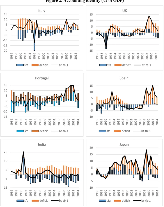
In addition, Figure 2 exemplifies the accounting identity for some countries, on a yearly basis, where we show the specific relevance and magnitude of the stock flow adjustment, which tend to be rather persistent over time in many cases, therefore blurring to some extent the link between (primary) budget balances and government debt dynamics.
[Figure 2]
For fiscal rules as well as their types and characteristics, we make use of the datasets created by the IMF. The first dataset was introduced by Schaechter et al. (2012) and its most recent available updates discussed in detail by Lledó et al. (2017). The rules are classified according to the following typology: expenditure rules (ER), revenue rules (RR), budget balance rules (BBR) and debt rules (DR). Additionally, we created a dummy variable FR_1, denoting the existence of any of these fiscal rules in a given country in a given year. Moreover, the dataset contains information on such features of the rules as existing escape clauses, enforcement procedures or independent monitoring councils or their transparency.
In the analysis, we include 65 countries, which had at least one of the rules in place during the period of analysis. Overall, during the 31 years of the timespan at least one rule in place
8
was observed in 1076 cases (on 2015 possible), the most frequent being the budget balance rule (974 cases), followed by debt rule (772 occurrences), expenditure rule (399), the least frequent being the revenue rule (186). Only a handful of countries (Germany, Indonesia, Japan, Malaysia, and Singapore) had at least one rule in place for the entire time span. In all of these cases, it was the balanced budget rule, additionally completed by an expenditure rule (for Germany) and debt rule (in Malaysia). If a given rule was in place, the debt rule was present in a given country for almost 16.5 years, balanced budget rule for 15.7 years, revenue rule for 13.3 years (but it was present only in 13 countries) and expenditure rule for 9.7 years. The dataset additionally contains information about monitoring, enforcement and escape clause for each type of rules. We use this data on somewhat more aggregate level, i.e., if any of the fiscal rules applied in a country had a monitoring of compliance in place, the variable FR_monitor assumes value 1 and zero otherwise. The same is the case for formal enforcement procedure and escape clauses whereas independent monitoring body and transparency are taken “as they are” from the IMF database.6
As far as fiscal rules are concerned we can plot the absolute number of new rules (of any type) over time by income group, and we get the pattern observed in Figure 3. Looking at Advanced Economies, while countries have implemented fiscal rules since the mid-1980s, most of them followed the Maastricht Treaty in 1992 (in adherence to the EU convergence criteria) as well as after the Global Financial Crisis. In non Advanced Economies, the absolute number of fiscal rules is lower than the advanced economies sample, and most of them were implemented starting in the early 2000s.
[Figure 3]
Gupta and Yläoutinen (2014) made available another dataset on fiscal rules, which we also use. They analyse fiscal institutional frameworks in G-20 economies complemented by six low-income countries (Kenya, Mozambique, Myanmar, Uganda, Vietnam and Zambia). In particular, aspects covered in this database include: fiscal reporting (fr), macro fiscal forecasting (mf), independent fiscal agency (ifa), fiscal objectives (fo), medium term budget framework
6 The most frequent and relatively persistent design feature is the existence of an enforcement mechanism, which
was in place in 28 countries on average for slightly more than 10 years. Marginally least popular is monitoring (25 countries, on average in place for 9.6 years), Transparency requirements were present in 21 countries, notably on average for the longest period, i.e. for almost 11 years. Independent monitoring body was in place in 22 countries, but as a relatively recent mechanism, its average duration only slightly exceeds 5 years. Finally, some form of escape clause is present in 12 countries, on average for 7.5 years.
9
(mbf), budget execution (be), understanding the scale and scope of the fiscal challenge (understanding), developing a credible fiscal strategy (developing) and implementing the fiscal strategy through the budget process (implementing). Except for ifa, which is present only in 17 out of the 26 countries, all of these institutions are to a smaller or larger extent present in at least 24 countries.7
4. Empirical Results
4.1. Baseline with Fiscal Rules
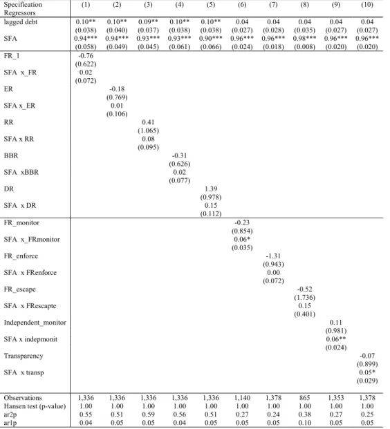
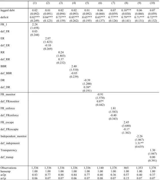
We start by estimating equations 4 and 5 for the different fiscal rules proxies using the entire sample of countries and time span. Results are displayed in Tables 1 and 2 respectively. Starting with Table 1, we observe that SFAs, as the accounting identity suggests, contribute to the change in the level of the debt-to-GDP ratio with a coefficient close to one. The existence of a fiscal rule leads of a fall in the debt level but the coefficient estimate is not statistically different from zero (specification 1). Since the coefficient on the SFA is not statistically different from one, the estimated coefficients on the interaction terms represent the covariances between the SFA and the deficit when a specific rule or a rule with a certain characteristic is in place. In the cases of the rules FRmonitor, indepmonit and transp the interaction term comes out positive but with a small magnitude and statistically significant at the 10 percent level. Contrary to the evidence presented in von Hagen and Wolff (2006) - who used a different definition for the fiscal rule dummy variable, closer to an event study approach, for a smaller country group - these findings suggest that fiscal rules in general did not led governments to systematically use SFAs to lower deficits in our sample of 65 countries. Moreover, in Table 2 we still have that fiscal rules do not statistically significantly affect the change in the debt level. As in Table 1, a positive covariance appears. An increase in the deficit by one percentage point is associated with an increase of the SFA by an amount between [0.4-1.3] depending on the fiscal rule proxy under scrutiny.
[Table 1] [Table 2]
10
4.2. Baseline with Fiscal Institutions
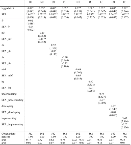
In Table 3 we re-estimate equations 4 and 5 using the smaller sample stemming from Gupta and Yläoutinen (2014) on fiscal frameworks. Still we obtain that in general fiscal rules did not significantly change the debt level in this group of 26 countries. Those countries containing a form of macro-fiscal forecasting tool (mf) seemed to have allowed governments to use SFAs to lower deficits (the interaction term is negative and statistically significant at the 5 percent level).
A better and improved expectational view of the economy and public finances, suggests that SFAs have become a policy variable to control the deficit in countries where such framework was in place. All other characteristics of the fiscal system do not seem to matter neither individually nor in conjunction with the SFA variable. Results from estimating equation 5 in this setting yield statistically insignificant coefficients and, as hence, are omitted for reasons of parsimony (but available upon request).
[Table 3] 4.3 Augmented Version with Fiscal Rules
In order to assess to what extent the cyclical component of the budget balance plays a role in the analysis, we have used the cyclical and cyclically adjusted parts of the budget deficit separately. Therefore, capturing the structural and cyclical dimensions of the deficit leads to the estimation of equation 6. Looking at Table 4 for the case of fiscal rule and our large expanded sample, both components of the deficit positively clearly affect the debt level, particularly the structural part. While expenditures rules seem to negatively affect the debt level (despite not being statistically significantly different from zero), its interaction with the cyclical component of the deficit yields a positive and statistically significant coefficient. This means that an increase in the cyclical deficit when expenditure rules are in place lead to an increase in debt. A similar conclusion is also true with regard to the debt rule, but in this case, the impact of both deficit components is similarly positive. Finally, the existence of fiscal rules in which monitor compliance exist, contributes to lower the debt level, but the cyclical deficit partly counteracts this desirable effect.
11
4.4 Country Sample and Time Split
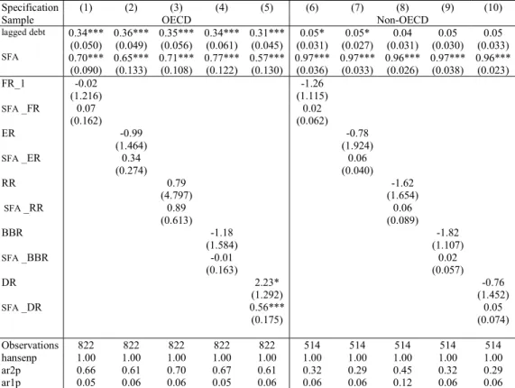
As a first sensitivity exercise, we split our large heterogeneous sample between OECD and non-OECD countries. We observe in Table 5 – estimating equation 4 – that SFAs seem to be more important in positively changing the debt level in non-OECD countries (where the coefficient estimates and closer to 1 vis-à-vis the OECD). In addition, we see that in the OECD sub-sample the existence of debt rules lead of a rise in the debt level, an effect that is exacerbated when coupled with SFAs.
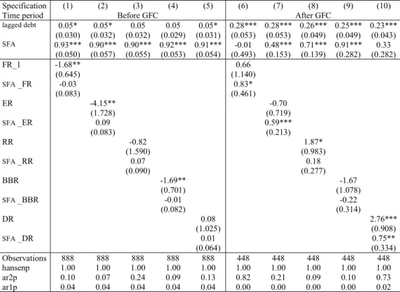
In addition, in Table 6 in turn, we split the period before and after the Global Financial Crisis (in 2018). The crisis was indeed a major structural break in the sense that before, most fiscal rules seem to lower debt levels and had a clear actively constraining role in keeping government debt from rising. The order of magnitude of the fall in the debt level due to the presence of fiscal rules before the crisis was between 1.7-4.2 percent of GDP. After the crisis, both revenue-based and debt-based rules starting contributing positively to the accumulation of debt, a fact that is reinforced with the existence of large SFAs.
[Table 5] [Table 6] 4.5 Other Robustness Exercises
Our final exercise relates to stress-testing our previous results to alternative estimators. In particular, we run a pooled OLS, a within fixed effects estimator and the bias corrected least squares dummy variable. Results in Table 7 confirm the relevance of SFAs for the change in government debt. Without accounting for potential endogeneity, we get the nice result that the simple existence of fiscal rules lowers the public debt level (specifications 1, 4, 7). In addition, as before, both components of the deficit positively affect public debt, with the positive effect of the structural component being reinforced when fiscal rules are present.
[Table 7]
In addition to the robustness check to alternative estimators, we also employed an alternative method to extract the structural and cyclical components of the budget deficit. In particular, instead of relying on the IMF’s WEO measure of output gap, we rather apply the recent filtering technique developed by Hamilton (2017). Once the output gap is obtained, we
12
then used it to get a new measure of the cyclically adjusted balance. Reflecting the fact that the elasticity of government revenues (REV) to output growth is close to one while expenditure (EXP) is largely inelastic to growth (Girouard and André, 2005), we multiply government revenues by the factor [1/(1+OG/100)] to get REV_adj (revenue adjusted), with OG being the output gap obtain via the Hamilton filter. Then CAB=REV_adj - EXP.8
The results from re-estimating equation 6 with system GMM and the new structural and cyclical deficit variables (and interaction terms) are not qualitatively different from the ones previously discussed (available upon request).
5. Conclusion and Policy Implications
We have assessed how SFA contribute to the path of the debt-to-GDP ratio in a panel of 65 countries in the period 1985-2014. Therefore, and vis-à-vis previous related literature, we extend the coverage beyond developed economies to include also emerging and low-income countries, an aspect previously unexplored. In addition to inspecting the role of fiscal rules in affecting SFAs, we go deeper in the analysis by looking at different types and design characteristics of those rules. Furthermore, for a subsample of countries, we also rely on a recent dataset on fiscal institutions and examine which matter the most for the build-up of SFAs.
Our main results are the following: i) SFAs contribute to the change in the level of the debt-to-GDP ratio with a coefficient close to one. ii) Fiscal rules in general did not led governments to a systematic use SFAs to lower deficits in our country sample. iii) Countries with some form of macro-fiscal forecasting tool in place have allowed governments to use SFAs to lower deficit. iv) The existence of fiscal rules in which monitor compliance exist, contributes to lower the debt level, although the cyclical deficit partly counteracts this desirable effect. v) The magnitude of the fall in the debt ratio due to the presence of fiscal rules before the crisis was between 1.7-4.2 percent of GDP. vi) After the GFC, both revenue-based and debt-based rules starting contributing positively to the accumulation of debt, a fact that is reinforced with the presence of large SFAs.
Our results have a number of policy implications. First, it is important to notice the effect of the GFC in reversing, to some extent, the performance of the fiscal rules in curbing government debt developments. Hence, policy makers would need to integrate this result in the implementation and redefinition of such fiscal frameworks. Second, the fact that in some cases countries used the SFA with an impact on the development of general government debt, raises
13
the issue of being cautious when perceiving the dynamics of the intertemporal government budget constraint essentially via the primary balance, implying the need to further transparency in that context, to ensure the mitigation of such SFA.
References
1. Abbas, S.M. Ali, Nazim Belhocine, Asmaa El-Ganainy and Mark Horton (2011), “Historical Patterns and Dynamics of Public Debt - Evidence From a New Database”, IMF Economic Review, 59(4), 717-742
2. Arellano, M., Bover, O. (1995), “Another look at the instrumental-variable estimation of errorcomponents models”. Journal of Econometrics 68, 29-52.
3. Blundell, R. and S. Bond (1998), “Initial Conditions and Moment Restrictions in Dynamic Panel Data Models,” Journal of Econometrics, 87, 115-143.
4. Bova E, Ruiz-Arranz M, Toscani F, and Ture H. (2016), “The Fiscal Costs of Contingent Liabilities: A New Dataset,” IMF Working Paper 16/14 (Washington: International Monetary Fund).
5. Bowsher, C.G. (2002), “On testing overidentifying restrictions in dynamic panel data models”. Economics Letters 77: 211–20.
6. Bruno, G. S. F. (2005), “Approximating the bias of the LSDV estimator for dynamic unbalanced panel data models”. Economics Letters 87: 361–366.
7. Campos, C. F.S., Jaimovich, D. and Panizza, U., (2006), “The unexplained part of public debt”, Emerging Markets Review, 7(3), 228-243,
8. Escolano, Julio (2010), “A Practical Guide to Public Debt Dynamics, Fiscal Sustainability, and Cyclical Adjustment of Budgetary Aggregates”, Technical Note, International Monetary Fund.
9. European Commission, DG for Economic and Financial Affairs (2003), “Public Finances in EMU 2003”. The European Commission, Brussels
10. Girouard, N. and C. André (2005), “Measuring Cyclically-adjusted Budget Balances for OECD Countries”, OECD, Economics Department, Working Paper, No. 434.
11. Gupta, S. and Yloutinen, S. (2014), “Budget institutions in Low-Income Countries: Lessons from G20”, IMF Working Paper 14/164, Washington DC.
12. Hamilton, J. (2017), “Why You Should Never Use the Hodrick-Prescott Filter,” NBER WP paper No. 23429.
13. Jaramillo, L., Mullas-Granados, C., Jalles, J. T. (2017), “Debt spikes, blind spots, and financial stress”, International Journal of Finance and Economics, 22 (4), 421-437.
14. Jaramillo, L., Mullas-Granados, C., Kimani, E. (2017). “Debt spikes and stock-flow adjustment: Emerging economies perspective”, Journal of Economics and Business, 94, 1-14. 15. Kiviet, J. F. (1995), “On bias, inconsistency, and efficiency of various estimators in dynamic panel data models”. Journal of Econometrics 68: 53–78.
16. Lledó, Victor, Sungwook Yoon, Xiangming Fang, Samba Mbaye, and Young Kim. (2017). Fiscal Rules at a Glance. March. Washington, DC: International Monetary Fund. 17. Milesi-Ferretti, G. (2003), “Good, bad or ugly? On the effects of fiscal rules with creative accounting”, Journal of Public Economics, 88, 1-2.
18. Roodman, D.M. (2009), “A note on the theme of too many instruments”. Oxford Bulletin of Economics and Statistics 71(1): 135–58.
19. Schaechter, A., T. Kinda, N. Budina, and A. Weber (2012), Fiscal Rules in Response to the Crisis – Toward the “Next Generation” Rules. A New Dataset. IMF Working Paper WP12/187. Washington, DC: International Monetary Fund.
14
20. von Hagen, J., and Wolff, G. (2006), “What Do Deficits Tell Us about Debt? Empirical Evidence on Creative Accounting with Fiscal Rules in the EU,” Journal of Banking and Finance, 30 (12), 3259–79.
21. von Hagen, J. (2002), “Fiscal Rules, Fiscal Institutions, and Fiscal Performance”, Economic and Social Review 33(3): 263-284.
22. Weber, A. (2012), “Stock Flow Adjustments and Fiscal Transparency: a cross-country comparison”, IMF Working Paper 12/39, Washington DC.
Figure 1. Total Stock Flow Adjustments in percent of 2014 GDP by country
-50 0 50 100 150 200 Sl ov ak R ep ub lic Cz ec h Re pu bl ic Isr ae l Po la nd Gr ee ce Lit hu an ia Bu rk in a Fa so M al ta Hu ng ar y Ne th er la nd s Ch ad M al i In di a Ec ua do r Ni ge r In do ne sia Ni ge ria Ne w Z ea la nd Cr oa tia Un ite d Ki ng do m Ca m er oo n Be lg iu m Ug an da M ex ico Un ite d St at es Ta nz an ia Po rt ug al Fr an ce Au st ra lia Be ni n Sp ai n Pa ki st an Pe ru Es to ni a La tv ia Rw an da M al ay sia Italy Se ne ga l Ru ss ia Ke ny a Sw ed en Au st ria Iran Ire la nd Sr i L an ka Br az il Ge rm an y De nm ar k Co lo m bi a Ch ile Ho ng K on g SA R Sw itz er la nd Sl ov en ia Ar ge nt in a Ur ug ua y Ca na da Cy pr us Lu xe m bo ur g Ic el an d Ja pa n Fi nl an d No rw ay Si ng ap or e pe rc en t o f 2 01 4 G DP
15
Figure 2. Accounting identity (% of GDP)
Note: “sfa” denotes stock flow adjustments; “deficit” denotes the budget deficit; “bt-bt-1” denotes the change in the public debt level.
Source: authors’ calculations.
-20 -15 -10 -5 0 5 10 15 19 86 19 88 19 90 19 92 19 94 19 96 19 98 20 00 20 02 20 04 20 06 20 08 20 10 20 12 20 14 Italy sfa deficit bt-tb-1 -15 -10 -5 0 5 10 15 19 86 19 88 19 90 19 92 19 94 19 96 19 98 20 00 20 02 20 04 20 06 20 08 20 10 20 12 UK sfa deficit bt-tb-1 -15 -10 -5 0 5 10 15 19 86 19 88 19 90 19 92 19 94 19 96 19 98 20 00 20 02 20 04 20 06 20 08 20 10 20 12 20 14 Portugal sfa deficit bt-tb-1 -10 -5 0 5 10 15 19 86 19 88 19 90 19 92 19 94 19 96 19 98 20 00 20 02 20 04 20 06 20 08 20 10 20 12 20 14 Spain sfa deficit bt-tb-1 -15 -5 5 15 25 19 86 19 88 19 90 19 92 19 94 19 96 19 98 20 00 20 02 20 04 20 06 20 08 20 10 20 12 20 14 India sfa deficit bt-tb-1 -10 -5 0 5 10 15 20 19 86 19 88 19 90 19 92 19 94 19 96 19 98 20 00 20 02 20 04 20 06 20 08 20 10 20 12 20 14 Japan sfa deficit bt-tb-1
16
Figure 3. Distribution of New Fiscal Rules implemented over time by Income Group
a) Advanced Economies b) Non-Advanced Economies
Source: International Monetary Fund’s fiscal rule dataset.
0 2 4 6 8 10 12 14 n u m b er 0 1 2 3 4 5 n u m b er
17
Table 1. Baseline, all countries, fiscal rules, equation (4), system GMM
Specification (1) (2) (3) (4) (5) (6) (7) (8) (9) (10) Regressors lagged debt 0.10** 0.10** 0.09** 0.10** 0.10** 0.04 0.04 0.04 0.04 0.04 (0.038) (0.040) (0.037) (0.038) (0.038) (0.027) (0.028) (0.035) (0.027) (0.027) SFA 0.94*** 0.94*** 0.93*** 0.93*** 0.90*** 0.96*** 0.96*** 0.98*** 0.96*** 0.96*** (0.058) (0.049) (0.045) (0.061) (0.066) (0.024) (0.018) (0.008) (0.020) (0.020) FR_1 -0.76 (0.622) SFA x_FR 0.02 (0.072) ER -0.18 (0.769) SFA x_ER 0.01 (0.106) RR 0.41 (1.065) SFA x RR 0.08 (0.095) BBR -0.31 (0.626) SFA xBBR 0.02 (0.077) DR 1.39 (0.978) SFA x DR 0.15 (0.112) FR_monitor -0.23 (0.854) SFA x_FRmonitor 0.06* (0.035) FR_enforce -1.31 (0.943) SFA x FRenforce 0.00 (0.072) FR_escape -0.52 (1.736) SFA x FRescapte 0.15 (0.401) Independent_monitor 0.11 (0.981) SFA x indepmonit 0.06** (0.024) Transparency -0.07 (0.899) SFA x transp 0.05* (0.029) Observations 1,336 1,336 1,336 1,336 1,336 1,140 1,378 865 1,353 1,378 Hansen test (p-value) 1.00 1.00 1.00 1.00 1.00 1.00 1.00 1.00 1.00 1.00
ar2p 0.55 0.51 0.59 0.56 0.51 0.27 0.24 0.38 0.27 0.25
ar1p 0.04 0.05 0.05 0.04 0.05 0.05 0.05 0.10 0.05 0.05
Note: Dependent variable is the change in debt in percent of GDP.Robust standard errors clustered at the country level in parenthesis. The Hansen test evaluates the validity of the instrument set, i.e., tests for over-identifying restrictions. AR(1) and AR(2) are the Arellano-Bond autocorrelation tests of first and second order (the null is no autocorrelation), respectively. A constant term has been estimated but it is not reported for reasons of parsimony. *, **, *** denote statistical significance at the 10, 5 and 1 percent levels, respectively. “FR_1” if a country has at least one fiscal rule; “ER” = expenditure rule in place; “RR” revenue rule in place; “DR” = debt rule in place; “BBR” = budget balance rule in place, “monitor” = at least one of the rules in place monitor compliance exist; “enforce” = at least one of the rules in place formal enforcement procedure exist; “escape” at least of the rules in place escape clause exist. “Independent_monitor” = an independent body monitors implementation of the rules. “transparency” = Fiscal Responsibility Laws are in place ensuring transparency and accountability.
18
Table 2. Baseline, all countries, fiscal rules, equation (5), system GMM
(1) (2) (3) (4) (5) (6) (7) (8) (9) (10) lagged debt 0.02 0.01 0.02 0.02 0.01 0.06 0.07 0.10*** 0.06 0.07 (0.092) (0.091) (0.094) (0.093) (0.092) (0.060) (0.059) (0.030) (0.060) (0.059) deficit 0.82*** 0.84*** 0.73*** 0.85*** 0.65*** 0.65*** 0.77*** 0.79*** 0.71*** 0.72*** (0.249) (0.123) (0.159) (0.262) (0.195) (0.137) (0.126) (0.141) (0.131) (0.132) FR_1 2.24 (1.658) def_FR 0.03 (0.244) ER 2.07 (1.423) def_ER -0.10 (0.269) RR 0.24 (1.803) def_RR 0.37 (0.232) BBR 2.40 (1.510) def_BBR -0.03 (0.239) DR -0.39 (1.200) def_DR 0.38* (0.191) FR_monitor -0.91 (1.570) def_FRmonitor 0.87* (0.442) FR_enforce 1.81 (1.583) def_FRenforce -0.40 (0.343) FR_escape 2.45 (3.680) def_FRescapte -0.17 (1.302) Independent_monitor -2.26 (1.867) def_indepmonit 1.31** (0.635) Transparency 1.30 (1.847) def_transp 0.00 (0.391) Observations 1,336 1,336 1,336 1,336 1,336 1,140 1,378 865 1,353 1,378 hansenp 1.00 1.00 1.00 1.00 1.00 1.00 1.00 1.00 1.00 1.00 ar2p 0.83 0.77 0.88 0.84 0.77 0.40 0.36 0.57 0.40 0.37 ar1p 0.06 0.07 0.07 0.06 0.07 0.08 0.07 0.15 0.07 0.07
Note: Dependent variable is the change in debt in percent of GDP. Robust standard errors clustered at the country level in parenthesis. The Hansen test evaluates the validity of the instrument set, i.e., tests for over-identifying restrictions. AR(1) and AR(2) are the Arellano-Bond autocorrelation tests of first and second order (the null is no autocorrelation), respectively. A constant term has been estimated but it is not reported for reasons of parsimony. *, **, *** denote statistical significance at the 10, 5 and 1 percent levels, respectively. “FR_1” if a country has at least one fiscal rule; “ER” = expenditure rule in place; “RR” revenue rule in place; “DR” = debt rule in place; “BBR” = budget balance rule in place, “monitor” = at least one of the rules in place monitor compliance exist; “enforce” = at least one of the rules in place formal enforcement procedure exist; “escape” at least of the rules in place escape clause exist. “Independent_monitor” = an independent body monitors implementation of the rules. “transparency” = Fiscal Responsibility Laws are in place ensuring transparency and accountability. Fiscal rules dataset from Lledó et al (2017).
19
Table 3. Baseline, all countries, fiscal institutions, equation (4), system GMM
(1) (2) (3) (4) (5) (6) (7) (8) (9) lagged debt 0.09* 0.09* 0.08* 0.09* 0.12* 0.08* 0.09* 0.09* 0.08* (0.045) (0.049) (0.046) (0.050) (0.059) (0.041) (0.047) (0.049) (0.046) SFA 1.01*** 1.02*** 0.98*** 1.04*** 0.99*** 0.98** 1.00*** 1.04*** 1.06*** (0.060) (0.018) (0.030) (0.036) (0.045) (0.357) (0.033) (0.032) (0.157) fr 0.92 (1.688) SFA_fr -0.04 (0.072) mf 0.20 (0.962) SFA _mf -0.11** (0.052) ifa 0.92 (1.584) SFA _ifa -0.06 (0.117) fo -0.20 (0.944) SFA _fo -0.12 (0.106) mbf -0.69 (1.700) SFA _mbf -0.05 (0.085) be 4.50 (3.338) SFA _be -0.01 (0.266) understanding 0.78 (1.427) SFA _understanding -0.07 (0.069) developing 0.07 (1.540) SFA _developing -0.09 (0.060) implementing 3.47 (2.884) SFA _implementing -0.07 (0.136) Observations 562 562 562 562 562 562 562 562 562 hansenp 1.00 1.00 1.00 1.00 1.00 1.00 1.00 1.00 1.00 ar2p 0.77 0.72 0.82 0.78 0.72 0.37 0.34 0.53 0.37 0.35 ar1p 0.06 0.07 0.07 0.06 0.07 0.07 0.07 0.14 0.07 0.07
Note: Dependent variable is the change in debt in percent of GDP. LDV denotes lagged dependent variable. Robust standard errors clustered at the country level in parenthesis. The Hansen test evaluates the validity of the instrument set, i.e., tests for over-identifying restrictions. AR(1) and AR(2) are the Arellano-Bond autocorrelation tests of first and second order (the null is no autocorrelation), respectively. A constant term has been estimated but it is not reported for reasons of parsimony. *, **, *** denote statistical significance at the 10, 5 and 1 percent levels, respectively. “fr”=fiscal reporting; “mf”=macro fiscal forecasting; “IFA”=independent fiscal agency; “fo” fiscal objectives; “MBF” medium term budget framework; “be” budget execution; “understanding”=understanding the scale and scope of the fiscal challenge; “developing” = developing a credible fiscal strategy; “implementing” = implementing the fiscal strategy through the budget process.
20
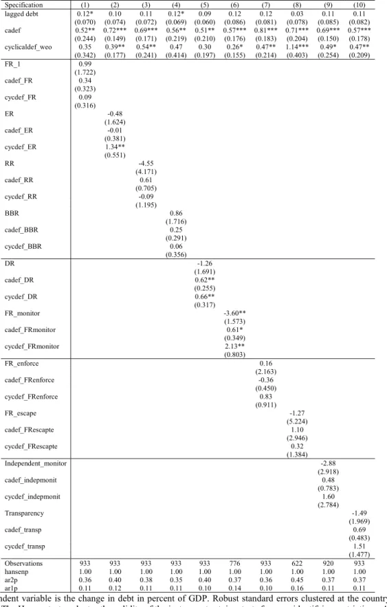
Table 4. Baseline Augmented, all countries, fiscal rules, equation (6), system GMM
Specification (1) (2) (3) (4) (5) (6) (7) (8) (9) (10) lagged debt 0.12* 0.10 0.11 0.12* 0.09 0.12 0.12 0.03 0.11 0.11 (0.070) (0.074) (0.072) (0.069) (0.060) (0.086) (0.081) (0.078) (0.085) (0.082) cadef 0.52** 0.72*** 0.69*** 0.56** 0.51** 0.57*** 0.81*** 0.71*** 0.69*** 0.57*** (0.244) (0.149) (0.171) (0.219) (0.210) (0.176) (0.183) (0.204) (0.150) (0.178) cyclicaldef_weo 0.35 0.39** 0.54** 0.47 0.30 0.26* 0.47** 1.14*** 0.49* 0.47** (0.342) (0.177) (0.241) (0.414) (0.197) (0.155) (0.214) (0.403) (0.254) (0.209) FR_1 0.99 (1.722) cadef_FR 0.34 (0.323) cycdef_FR 0.09 (0.316) ER -0.48 (1.624) cadef_ER -0.01 (0.381) cycdef_ER 1.34** (0.551) RR -4.55 (4.171) cadef_RR 0.61 (0.705) cycdef_RR -0.09 (1.195) BBR 0.86 (1.716) cadef_BBR 0.25 (0.291) cycdef_BBR 0.06 (0.356) DR -1.26 (1.691) cadef_DR 0.62** (0.255) cycdef_DR 0.66** (0.317) FR_monitor -3.60** (1.573) cadef_FRmonitor 0.61* (0.349) cycdef_FRmonitor 2.13** (0.803) FR_enforce 0.16 (2.163) cadef_FRenforce -0.36 (0.450) cycdef_FRenforce 0.83 (0.911) FR_escape -1.27 (5.224) cadef_FRescapte 1.10 (2.946) cycdef_FRescapte 0.32 (1.384) Independent_monitor -2.88 (2.918) cadef_indepmonit 0.48 (0.783) cycdef_indepmonit 1.60 (2.784) Transparency -1.49 (1.969) cadef_transp 0.69 (0.483) cycdef_transp 1.51 (1.477) Observations 933 933 933 933 933 776 933 622 920 933 hansenp 1.00 1.00 1.00 1.00 1.00 1.00 1.00 1.00 1.00 1.00 ar2p 0.36 0.40 0.38 0.35 0.40 0.37 0.36 0.45 0.37 0.37 ar1p 0.11 0.12 0.11 0.11 0.10 0.14 0.10 0.16 0.11 0.11
Note: Dependent variable is the change in debt in percent of GDP. Robust standard errors clustered at the country level in parenthesis. The Hansen test evaluates the validity of the instrument set, i.e., tests for over-identifying restrictions. AR(1) and AR(2) are the Arellano-Bond autocorrelation tests of first and second order (the null is no autocorrelation), respectively. A constant term has been estimated but it is not reported for reasons of parsimony. *, **, *** denote statistical significance at the 10, 5 and 1 percent levels, respectively. “FR_1” if a country has at least one fiscal rule; “ER” = expenditure rule in place; “RR” revenue rule in place; “DR” = debt rule in place; “BBR” = budget balance rule in place, “monitor” = at least one of the rules in place monitor compliance exist; “enforce” = at least one of the rules in place formal enforcement procedure exist; “escape” at least of the rules in place escape clause exist. “Independent_monitor” = an independent body monitors implementation of the rules. “transparency” = Fiscal Responsibility Laws are in place ensuring transparency and accountability. Fiscal rules dataset from Lledó et al (2017).
21
Table 5. Baseline, OECD vs non-OECD, fiscal rules, equation (4), system GMM
Specification (1) (2) (3) (4) (5) (6) (7) (8) (9) (10)
Sample OECD Non-OECD
lagged debt 0.34*** 0.36*** 0.35*** 0.34*** 0.31*** 0.05* 0.05* 0.04 0.05 0.05 (0.050) (0.049) (0.056) (0.061) (0.045) (0.031) (0.027) (0.031) (0.030) (0.033) SFA 0.70*** 0.65*** 0.71*** 0.77*** 0.57*** 0.97*** 0.97*** 0.96*** 0.97*** 0.96*** (0.090) (0.133) (0.108) (0.122) (0.130) (0.036) (0.033) (0.026) (0.038) (0.023) FR_1 -0.02 -1.26 (1.216) (1.115) SFA _FR 0.07 0.02 (0.162) (0.062) ER -0.99 -0.78 (1.464) (1.924) SFA _ER 0.34 0.06 (0.274) (0.040) RR 0.79 -1.62 (4.797) (1.654) SFA _RR 0.89 0.06 (0.613) (0.089) BBR -1.18 -1.82 (1.584) (1.107) SFA _BBR -0.01 0.02 (0.163) (0.057) DR 2.23* -0.76 (1.292) (1.452) SFA _DR 0.56*** 0.05 (0.175) (0.074) Observations 822 822 822 822 822 514 514 514 514 514 hansenp 1.00 1.00 1.00 1.00 1.00 1.00 1.00 1.00 1.00 1.00 ar2p 0.66 0.61 0.70 0.67 0.61 0.32 0.29 0.45 0.32 0.29 ar1p 0.05 0.06 0.06 0.05 0.06 0.06 0.06 0.12 0.06 0.06
Note: Dependent variable is the change in debt in percent of GDP. Robust standard errors clustered at the country level in parenthesis. The Hansen test evaluates the validity of the instrument set, i.e., tests for over-identifying restrictions. AR(1) and AR(2) are the Arellano-Bond autocorrelation tests of first and second order (the null is no autocorrelation), respectively. A constant term has been estimated but it is not reported for reasons of parsimony. *, **, *** denote statistical significance at the 10, 5 and 1 percent levels, respectively. “FR_1” if a country has at least one fiscal rule; “ER” = expenditure rule in place; “RR” revenue rule in place; “DR” = debt rule in place; “BBR” = budget balance rule in place.
22
Table 6. Baseline, before vs after GFC, fiscal rules, equation (4), system GMM
Specification (1) (2) (3) (4) (5) (6) (7) (8) (9) (10)
Time period Before GFC After GFC
lagged debt 0.05* 0.05* 0.05 0.05 0.05* 0.28*** 0.28*** 0.26*** 0.25*** 0.23*** (0.030) (0.032) (0.032) (0.029) (0.031) (0.053) (0.053) (0.049) (0.049) (0.043) SFA 0.93*** 0.90*** 0.90*** 0.92*** 0.91*** -0.01 0.48*** 0.71*** 0.91*** 0.33 (0.050) (0.057) (0.055) (0.053) (0.054) (0.493) (0.153) (0.139) (0.282) (0.282) FR_1 -1.68** 0.66 (0.645) (1.140) SFA _FR -0.03 0.83* (0.083) (0.461) ER -4.15** -0.70 (1.728) (0.719) SFA _ER 0.09 0.59*** (0.083) (0.213) RR -0.82 1.87* (1.590) (0.983) SFA _RR 0.07 0.18 (0.090) (0.277) BBR -1.69** -1.67 (0.701) (1.078) SFA _BBR -0.01 -0.22 (0.082) (0.314) DR 0.08 2.76*** (1.025) (0.908) SFA _DR 0.01 0.75** (0.064) (0.334) Observations 888 888 888 888 888 448 448 448 448 448 hansenp 1.00 1.00 1.00 1.00 1.00 1.00 1.00 1.00 1.00 1.00 ar2p 0.10 0.07 0.24 0.09 0.13 0.82 0.21 0.09 0.10 0.73 ar1p 0.04 0.04 0.04 0.04 0.04 0.00 0.00 0.00 0.00 0.02
Note: Dependent variable is the change in debt in percent of GDP. Robust standard errors clustered at the country level in parenthesis. The Hansen test evaluates the validity of the instrument set, i.e., tests for over-identifying restrictions. AR(1) and AR(2) are the Arellano-Bond autocorrelation tests of first and second order (the null is no autocorrelation), respectively. A constant term has been estimated but it is not reported for reasons of parsimony. *, **, *** denote statistical significance at the 10, 5 and 1 percent levels, respectively. “FR_1” if a country has at least one fiscal rule; “ER” = expenditure rule in place; “RR” revenue rule in place; “DR” = debt rule in place; “BBR” = budget balance rule in place.
Fiscal rules dataset from Lledó et al (2017).
Table 7. Robustness to other estimations, equations (4, 5 ,6)
Specification (1) (2) (3) (4) (5) (6) (7) (8) (9)
Estimator OLS OLS OLS FE FE FE LSDV LSDV LSDV
Equation Eq.4 Eq.5 Eq.6 Eq.4 Eq.5 Eq.6 Eq.4 Eq.5 Eq.6
lagged debt 0.16*** 0.10 0.19* 0.12*** 0.02 0.07 0.01 -0.13*** -0.06 (0.040) (0.091) (0.108) (0.029) (0.088) (0.092) (0.026) (0.040) (0.054) SFA 0.88*** 0.98*** 0.99*** (0.057) (0.037) (0.017) FR_1 -1.04*** 0.83 0.35 -1.14*** 1.58* 0.86 -0.85 1.79*** 0.89 (0.282) (0.700) (0.476) (0.230) (0.927) (0.936) (0.537) (0.513) (0.784) SFA _FR -0.08 -0.00 0.00 (0.076) (0.042) (0.024) deficit 0.45*** 0.87*** 0.94*** (0.127) (0.156) (0.099) def_FR 0.16 0.07 0.05 (0.124) (0.123) (0.099) cadef 0.35*** 0.69*** 0.75*** (0.098) (0.121) (0.149) cyclicaldef_weo 0.26* 1.05*** 1.19*** (0.160) (0.267) (0.254) cadef_FR 0.23** 0.35*** 0.35** (0.101) (0.122) (0.157) cycdef_FR 0.15 -0.21 -0.22 (0.187) (0.228) (0.220) Observations 1,336 1,336 933 1,336 1,336 933 1,336 1,336 933 R-squared 0.68 0.16 0.21 0.82 0.25 0.32 0.85 0.22 0.26
Note: Dependent variable is the change in debt in percent of GDP. Robust standard errors clustered at the country level in parenthesis. The Hansen test evaluates the validity of the instrument set, i.e., tests for over-identifying restrictions. AR(1) and AR(2) are the Arellano-Bond autocorrelation tests of first and second order (the null is no autocorrelation), respectively. A constant term has been estimated but it is not reported for reasons of parsimony. Specifications 4-6 include country and time fixed effects omitted for reasons of patrimony. *, **, *** denote statistical significance at the 10, 5 and 1 percent levels, respectively. “FR_1” if a country has at least one fiscal rule; “ER” = expenditure rule in place; “RR” revenue rule in place; “DR” = debt rule in place; “BBR” = budget balance rule in place.
23
APPENDIX
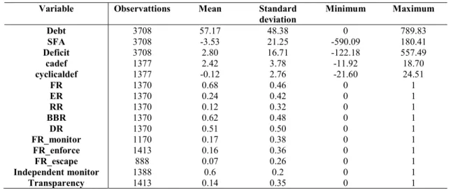
Table A1. Summary Statistics
Variable Observattions Mean Standard
deviation Minimum Maximum Debt 3708 57.17 48.38 0 789.83 SFA 3708 -3.53 21.25 -590.09 180.41 Deficit 3708 2.80 16.71 -122.18 557.49 cadef 1377 2.42 3.78 -11.92 18.70 cyclicaldef 1377 -0.12 2.76 -21.60 24.51 FR 1370 0.68 0.46 0 1 ER 1370 0.24 0.42 0 1 RR 1370 0.12 0.32 0 1 BBR 1370 0.62 0.48 0 1 DR 1370 0.51 0.50 0 1 FR_monitor 1170 0.17 0.38 0 1 FR_enforce 1413 0.16 0.36 0 1 FR_escape 888 0.07 0.26 0 1 Independent monitor 1388 0.6 0.2 0 1 Transparency 1413 0.14 0.35 0 1