DOI: http://dx.doi.org/10.1590/1980-5373-MR-2017-0238
Materials Research. 2017; 20(5): 1432-1443 © 2017
Determination of Surface Temperature in ICP RF Plasma Treatments of Organic Materials
Carlos Eduardo Fariasa, Euclides Alexandre Bernardellia, Paulo Cesar Borgesa, Márcio Mafraa*
Received: March 01, 2017; Revised: May 30, 2017; Accepted: July 12, 2017
The reactions that can occur on organic materials treated in plasma enviorement are strongly afected by surface temperature, thus the sharp determination of this variable is extremely important to process control. In situ temperature measurements are often employed; however, the measured point
is generally under the treated surface. If in metallic materials the high thermal conductivity minimizes this problem, in non-metallic materials processing it becomes important, because its thermal resistivity besides a high sensibility to small temperature variations. The present work uses a simulation tool to extract thermal data on Ar+O2 RF plasma processing of Stearic Acid. Experimental data were obtained
by thermocouples placed inside the samples. The extrapolation of surface temperature was performed by numerical simulation with Autodesk CFD software v.15.1. Results show that the temperature of the surface reaches values higher than the ones measured inside the sample holder. This diference of temperature is in good agreement with the visual observation of the phase transformations in the treated material, showing a simple and valuable tool to better control of plasma treatments.
Keywords: Ultimate surface temperature, RF plasma treatment, Temperature simulation.
* e-mail: [email protected]
1. Introduction
It is already common knowledge, by thermodynamic laws and Arrhenius equation, that the material's temperature inluences its reactivity with the environment, either in kinetic form (reaction rate), in the form of activation energy (heat required to allow the beginning of a reaction)1, surface
temperature for processes like etch rate2, deposition rate3-5,
or polymerization4,6 of the materials exposed to plasmas.
However, there are cases in which is necessary to avoid the occurrence of speciic reactions by controlling the reached temperature on materials surface, such as in food sterilization processing that degrades the lavor in higher temperatures7,
controlled solidiication8, precipitation of unwanted second
phases in metal alloys, grain growing, and phase change in ceramics9. Therefore, many works were conducted with
techniques that would allow the measurement of this variable in surface treatments, especially in plasma systems.
In cleaning and degradation plasma processes, where speciic reactions of organic compounds depends on the temperature10,11, the correct analysis of this variable is very
important. Previous works found that when stearic acid heats due to reactions with plasma, it melts and this leads to many undesirable efects, such as the formation of resistant compounds and boiling. It has already been evidenced that in relatively high temperatures (313 K)12,13, even when the
material begins in the solid state, functionalization reactions becomes more important than degradation, leading to polymerization processes. On the other hand, treatments at lower temperatures (273 K) lead to high mass loss, where
the possible by-products of functionalization are removed in degradation processes10.
On most studies of plasma degradation, the temperature measurement was obtained by a thermocouple, which is placed into the sample holder or into the sample itself. However, the exposed surface reacts with the plasma active species and could reach higher temperatures than those measured. Also, simply placing the tip of the thermocouple exactly on the surface is not an eicient method because plasma species could interact with the metallic tip, heating it more than the sample14.
Knoerzer7 examined many diferent temperature measurement
techniques like thermocouple, resistance thermometer, thermal-paper (also found in15 and16), autoclave tape and a
iber-optic sensor. Among all these techiniques, he found that iber-optic system was a reliable method since it did not sufer from the heating efect of charged particles from the discharge. However, some plasma reactors do not allow the easy placement of this kind of iber inside the chamber.
Galvão17 and Leal18 have extrapolated the surface
temperature of a steel AISI M35, analyzing its microstructure and hardness along the thickness of this metal exposed to plasma. They concluded that on a microlayer of surface material, the temperature could be more than 100 K higher than the bulk.
Salter and Amiel19,20 have used infrared cameras to
analyze the surface temperature of materials treated under special plasma and laser conditions. Salter19 observed that
temperature by IR camera was slightly higher than the one measured above the subtract with a thermocouple. However, not every system allows the visualization of a sample surface temperature and still needs other approaches to reach a correct value.
Akamatsu8 and Osch21 used experimental methods and
numerical analysis to extrapolate values to extreme conditions of samples exposed to ion implantation and lasers, working with very high temperatures and shorter times. In those cases, errors of tens of degrees are easily acceptable. However, when working with cold plasma systems, this kind of error could mean very diferent material behaviors.
On most systems, the use of thermocouples to measure temperature inside a subtract is acceptable due to a good heat conductivity of the subtract and the simplicity of setup. On the other hand, when the heat conductivity of treated materials is low, as in polymer and other organic molecules processing, simply using a thermocouple inside a substact holder is not enough because these materials are very sensitive to small temperature variations on its surface.
Previous works on RF discharge by Farias10, DC and
after-glow by Bernardelli12,22 and Mafra13, used thermocouples
inside the crucible and inside the sample, respectively. However, since reactions between sample and plasma generated species happen on the surface and the sample has a thickness of about a few millimeters, at least at the beginning of the treatment, there should be a delay on temperature measurements. Therefore, the present work present a way to achieve a most accurate value of surface temperature, by combining the thermocouple measurements into the sample and numeric simulation of the temperature at plasma-sample interface.
2. Materials and Method
2.1 Experimental setup
The experimental setup is depicted in Figure 1. Figure 1a shows the plasma reactor, which consists of a borosilicate tube with 34 mm inner diameter, 650 mm length and 2 mm thickness. The plasma is generated by a copper coil with 9 turns, connected to a radio frequency power source Tokyo Hi-Power, RF-300 model (and a matching box model MB-300), with a frequency of 13.56 MHz, which was used with the ixed power of 50 W (400 V peak-to-peak). The atmosphere is composed by a gas mixture of Ar-10vol% O2
lowing at 750 sccm at pressure of 1.5 Torr.
A temperature control system[1] (TCS) consisting of
water recirculation (pumped at 95 L/h), covering 110 mm of the discharge tube length, was used. The sample holder is made of poly-tetraluoroethylene, and its design and dimensions are shown in Figure 1b. A 4 mm deep itting groove is provided to place the sample. The curved face of the sample holder is shaped to allow good coupling between
the sample holder and the glass tube. The work material was 95% pure Stearic Acid (S.A.), because it is a standard molecule to plasma degradation studies. It was placed on the sample holder in a molten state, until a small amount was above the surface. When solidiied, the excess of S.A. was scraped with the aid of a metallic blade, to produce a lat surface. Due experimnental setup, it is not possible to move or visualize the sample during treatment as in many other plasma reactors. However, this material has a melting point at 341 K that will be used as a temperature indicator.
The thermocouple (Type K) can be placed at two diferent positions, always at 7 mm above the base of the sample holder (in central line), and penetrating the sample holder approximately 12 mm, from the front or back sides. Due to RF ield of plasma source, there was some interference in the thermocouple measurements. These were observed as a constant increase in reading value while the RF source remained on. After several adjustments in the coniguration, position and electrical insulation of the equipment, the increment was reduced to diferences smaller than 2 K. After each experiment, when the RF source was turned of, the value of the diference in the temperature reading was noted and used to correct the data.
The sample holder was placed in the central position of TCS in all experiments. The model used for the simulation corresponds to a section of 10 mm length of the front and back positions of the sample holder, with the glass, as shown in Figure 1c.
Each experiment was repeated four times, and the error bars are calculated as a conidence interval of 95%.
2.2 Experimental and simulation setup
The parameters of the experiments can be seen in Table 1. In order to determine the contact resistance between the sample holder and the discharge tube (Condition 1), a sample was placed initially at 293 K in the central position of TCS, and the pressure was reduced to 0.01 Torr to inhibit thermal exchanges other than conduction. Heat exchange by radiation was not considered in this system due to the low temperature diferences between sample and the TCS, and the short time for cooling or heating. In these experiments, the TCS contained water at temperatures of 273 and 313 K (for heating and cooling, respectively) and the evolution of the sample temperature was recorded every 1/3 minute until stabilization. Simulations have shown TCR values of 0,007 and 0,013 K.m/W, for heating and cooling, respectively.
To begin the experimental analysis (Condition 2), the temperature of the sample was controlled at 273, 293 or 313 K (stabilized for 30 minutes under vacuum), considering these values as the initial temperature. After that, the plasma was turned on and the temperature was measured at every 20 second up to 12 minutes of exposure. Because of diferent behaviors in the front and the back of the sample, analysis was made on both positions and the results were discussed.
Farias et al.
1434 Materials Research
Figure 1. (a) Experimental Setup, (b) Detail of sample holder (dimensions in mm), (c)
Three-dimensional model used for simulation
Table 1. boundary conditions for simulations.
Condition 1 Condition 2 Condition 3
Regime Transient Transient Transient
Type Experimental and Simulation Experimental and Simulation Simulation
Time (min) 0 - 20 0 - 12 0 - 12
Position Thermocouple Thermocouple Surface
TCS temperature.(ixed) (K) 273; 313 273; 293; 313
Initial temp. (K) 293 273; 293; 313
Heat generation No Yes
TCR (K.m.W-1) Unknow R1; RM; R2
Number of samples 4 4 in the front position 4 in the back position
R1, R2: thermal contact resistance values obtained by simulation 1 on back and front position; RM: average value of the thermal contact
resistance R1 and R2
After the measurements, simulations were carried out, beginning from a system without heat generation on the surface, and by trial, adding heat generation values on the surface to it the simulated curves to the experimental results.
Using the boundary values, heat generation on the surface, TCR and diferent initial temperatures (273, 293 and 313 K) obtained under Condition 2, the temperature curve on the surface was extracted.
The values obtained are validated by two methods. First, since the melting temperature of S.A. is 341 K, when
the surface reaches this value, melting spots should appear on the surface. To observe these physical changes in the samples, a series of experiments were made, removing the samples from the reactor after 2, 4, 6, 8, 10 and 12 minutes of treatment, for each initial temperature.
2.3 Material data
Table 2 lists the properties of materials used for the simulation.
Table 2. Data of materials used23,24.
Density (g/cm3)
Thermal
Conductivity Coeicient (W.m-1.K-1)
Melting Temperature
(K)
Glass
(borosilicate) 2,7 1,10
-PTFE 2,16 0,25 600
S.A. 0,94 0,30 341
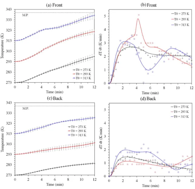
than the back position to all respective onset temperatures. The highest heating on the front position was 26±3 K, while on the back position, it was 13±2 K. This diference could be related to a higher consumption of reactive species at the front position, leaving a lower concentration to interact with the surface at the back position, according to the gas low.
The temperature at the front position of the sample with onset at 313 K showed values almost equivalent between minutes 4 to 6 of treatment. It can be attributed to the sample melting in a position close to the thermocouple. If the SA properties are considered, Falleiro25 has shown that melting temperature of this substance is almost constant in relation to the pressure inside the vacuum chamber. On the other hand, Belmonte26 have observed the melting of hexatriacontane and
stearic acid samples exposed to Ar-O2 afterglow and, under
his conditions, melting was attributed to physical-chemical transformation reactions leading to changes in the nature of the sample. Indeed, these transformations also occurs in the present work, as will be presented later.
In almost all cases, it takes approximately 2 minutes to increase the temperature of the thermocouple in 2 K. However, as it will be seen later on this paper, this amount of time is enough to produce molten material with onset of 313 K, as indicative of a considerable higher surface temperature and/or structural and chemical transformations of the sample with the plasma exposition.
To highlight small changes in the heating process that are not clearly visible in a temperature vs. time curve, derivative of temperature with time was used to reproduce the experimental measurements, visible at Figures 2 (b) and (d). In a thermal system based on conduction with heat generation, the existence of diferent proiles of heating rate (dT/dt), during the treatment, indicate the occurrence of diferent phenomena or change in heat generation. To the sample at onset of 273 K, in both front and back positions, the heating rate rapidly increase until it reaches a maximum value at approximately 3 minutes of treatment, decreasing slowly after that.
In an ideal system, if no physical-chemical modiications occur, a constant temperature proile could be reached after a long time of treatment, and the heating would reach dT/dt=0. If on the back position this tendence is observed, in front position, from 6 to 10 minutes of treatment, the heating is almost constant. It means that something had changed on the surface and more heat is being produced at this point. This behavior could be related to the own heating of the sample, which favors the reactivity and, therefore, it increases the heat generation and transfer.
At 293 K, there is also a rapid heating at the beginning, but it lasts until 4 minutes on the front position and until 2 minutes on the back. At the front position, there is a peak of heating that last only a few seconds. Since this event happened to all samples under this condition at the same period, this outlier point was considered on the simulation. Two possible explanations were found to account for this behaviour. First, Bernardelli12 showed that atomic oxygen
2.4 Boundary conditions and considerations
All simulations were performed using a simple transient thermal conduction model with contact resistance between sample holder and glass, at Autodesk CFD simulation software, version 15.1. This software uses a model called Compact Thermal Model that uses inite elements nodes to calculate transient heat transfer. In software, only material properties and boundary conditions were input while all speciic variables of simulation were kept as default of software.
The meshing were created with at least 7500 nodes distributed over the model. The simulation was created with at least 3 interactions per second, and data was saved at each 5 second. All simulated data was extracted direct from the software, by selecting a point of interest and extracting the evolution of the temperature on that point.
All simulation were purely heat transfer by conductivity, without considering radiation (due low temperature diference between sample and environment) and convection (vacuum environment) heat transfer modes. In the used software, it was not possible to consider phase changing of material and so, absolut values of surface temperature after melting of material may not be correct, but should be close enough. This phase changing of material will be used as a temperature indicator.
As is the objective of this paper, the surface temperature will be an extrapolated value from simulation, based on what was designed to obtain a heating proile at thermocouple position.
3. Results and Discussion
3.1 Experimental measurements during plasma
treatment
Farias et al.
1436 Materials Research
Figure 2. Experimental measurements of temperature in the region of thermocouple for the front position (a) and its instant variation
measured (signals) and simulated (line) (b); measured temperature in the backt position (c) and its instant variation measured (signals) and simulated (line) (d). The dashed line indicates the value for the melting temperature (M.T.) of S.A.
active species are able to difuse during liquid phase, and promote reactions, increasing the heating of the sample at the moment. At the same time, Tagawa27,28 found that when
polymers are exposed to atomic oxygen and UV light, the angle of incidence can increase the rate of interaction considerably. However, since the increase on the incident angle due the melt puddle of SA is minimal on experimental conditions, the efect of the presence of a liquid phase on SA is considerably more important to the heating.
After this peak at 293 K, the heating slow down to a plateau where then it is kept constant for approximately 1 minute, and then it starts to slowly decrease until the end of treatment. After a long exposure with the material on liquid phase (about 40 minutes), Mafra13 and Bernardelli12 observed
a decrease on the sample temperature due to oxygen saturation of the molten puddle and structural changes on the treated material. It is worth to remember that in the present work the sample was immersed in the discharge, thus it is submitted to the impingement of charged species. These collisions can heat the sample and can produce chain scission, which also contributes to the occurrence of liquid phase.
phase on the surface, which will be better understood from the visual analysis presented later.
At 313K there are no visible peaks of heating that could be related to the melting of the sample. However, individually analyzing experimental data from all samples at 313 K, there was a small peak of heating for each sample, but smaller, and at diferent times, which were masked by data averaging and it is the result of a more aggressive treating condition. As it will be seen later, it is again related to the beginning of the sample's melting. Between 3 and 5 minutes, on the front position, heating decreases rapidly, almost reaching 0 K/min at 5 minutes; this behavior was associated to the melting of the material around the thermocouple. After this point, the front position heats again, reaching a second maximum value at 9 minutes and only decreasing after that. On the back position, after the maximum value at 3 minutes, the system keep a constant heating until 6 minutes and it starts to decrease until the end of experiment.
An interesting observation about the simulation process relates to the generated heat to all samples. A main result obtained by the successive approximations to achieve the best it is that any modiication on the heating measured on the thermocouple, in this system, happened on the surface, between 40 seconds to 1 minute before the event. As an example, the heating peak at the front position with onset at 293 K, happened at 4 minutes and 20 seconds while on simulation, the generated heating peak had to happen at 3 minutes and 40 seconds on the surface to reproduce a peak at the thermocouple position. Thus, it is reasonable to say that, on this kind of system, there is a delay between the surface event and the response on the measuring system as it should happen on others systems that uses thermocouples under sample holder.
3.2 Simulation on the surface
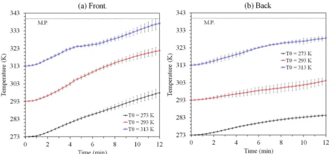
Figure 3 shows the simulated temperature proiles of a selected point on the surface, located on the central axis of the sample to the front (3a) and back (3b) posiotions. In all cases, simulation shows that the temperature increases very quickly on surface when compared with the measured point (on the thermocouple). This high heating rate is a situation that is already known when treating organic molecules in oxygenated plasmas, as shown by Praveen et. al29 on their
work; even a short exposure to oxygen plasmas, of less than 1 minute, was enough to heat lignocellulosic natural coir ibers to a temperature where it degrades. On this study, the amount of power and oxygen concentration applied were considerably lower, and also, the TCS system provided an eicient way to heat the extraction of sample, lowering the material's reactivity with plasma and, then, making it possible to analyze the temperature curve.
In all cases, the measured temperature on thermocouple takes more than 2 minutes to increase approximately 2 K,
while the simulation shows that, on the surface, it takes 6 seconds (or less) to increase the same amount. This is obviously related to the fact that the only source of heating of this system is located at the surface (by the interaction plasma-sample), and the low thermal conductivity of both the crucible and the sample.
Absolute values of temperature variation at the end of simulation are 73, 77 and 74 K at the front, and 29, 38 and 41 K at the back for the onsets of 273, 293 and 313 K, respectively. Those values are much higher than the measured ones on the thermocouple, meaning that in treatments of organic materials in oxidative plasmas, a great attention need to be devoted to temperature measurements, to avoid undesirable reactions and/or misinterpretations of results. This high temperature is in accordance with the results found by Mafra30, where exothermal reactions between Ar-O
2 late
afterglow were strong enough to heat the gas downstream. In the present work, where the sample is placed into the discharge, and, because of the energetic collisions that will take place, a more important heating is expected.
At the front position, all samples achieved on the surface, temperatures that are higher than the melting of SA. This occurred at 10 min and 40 sec to sample with onset at 273 K, 4 minutes for onset of 293 K and at 50 seconds to the onsets of 313 K. In respect to the derivate of those curves, it is visible that the higher it is the onset, the faster it increases its temperature with time, at least on the irst minute of exposition.
It is also observable that the heating peak at the front position of the sample with onset at 293 K takes place right after its surface reaches the SA's melting temperature. One could relate this phenomenon with the melting of the sample surface, due to previous explanations that the reactivity of the material increases with the formation of the liquid phase. However, this condition only appears with the onset of 293 K, and under other conditions, it is believed that there was not a good balance of heat conduction and heat generation to create a visible heating peak. At 273 K, the melting only occurs after 10 minutes and, at that time, the heat generated is already well distributed through the sample and a heating peak was not well detected. At 313 K, the reactions were really fast and this creates a condition where the heat peak happened but changed considerably to each sample, and it was masked due to averaging between the other samples.
Farias et al.
1438 Materials Research
Figure 3. Temperature simulation on the surface at the front (a) and back (b) positions, in relationship to the gas low. The dot line
represents the melting temperature of the sample.
Figure 4. Simulated temperature for the interface region between
SA and the sample holder for the front position with onset at 313 K. The dot line represents the melting temperature of the sample.
In accordance with the hypothesis, the temperature on this region was kept close to the melting temperature of SA during the entire time that the generated heat in this condition remained at its lowest plateau. Therefore, the latent heat of fusion is a very important variable to consider at simulation. However, due to software limitations, it was not possible to consider this variable. For this reason, the absolute temperature of the surface after melting must be measured with caution.
On the back position, the only condition that exceeds the M.T. line is the one with onset at 313 K at 2 minutes and 20 seconds. The increase on the heating of the onset at 293 K after 8 minutes, at a temperature considerably lower than
the melting point, is not related to the phase transformation of the surface, with another source of heat being necessary to produce this phenomenon.
3.3 Validation of simulation 1 (visual analysis)
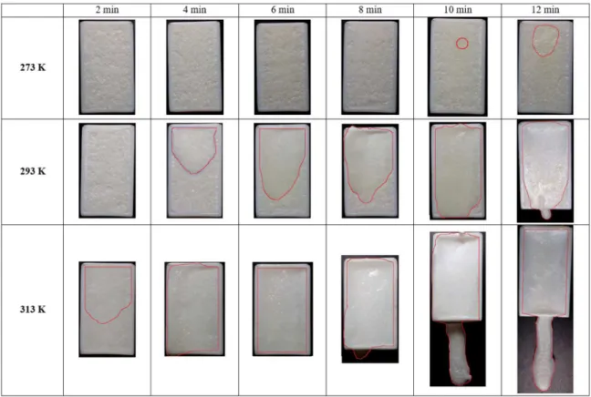
Samples from this topic were prepared only after the results of simulations had been completed. Thus, the results of this topic serve to validate the simulation related to with when and where melting of surface would occur. Figure 5 shows the results.
Starting with sample with onset at 273 K, after 10 minutes of treatment, a small puddle of molten material appear on the surface of the front position. Later on, this puddle only increases in size. This result is rigorously in accordance with Figure 3 (a) for the same onset. On the back position, no sign of melting appears on the surface, also in agreement with Figure 3 (b) for the same onset. It was also observable, that after 6 minutes of treatment, there is a weak yellowing of the surface (not so visible on the pictures due to light efects of the camera), that is a clear sign of chemical modiications of the organic compound due oxidation from plasma31,32.
Figure 5. Sample images during experiment at diferent onset temperatures. Sample positioning on picture is up = front position, down
= back position, relative to gas low.
phenomena, which will certainly happen, can also contribute to the appearance of the molten material.
Looking at the pictures in Figure 5, with onset at 293 K, one could believe that after 6 minutes there was already molten material on the surface of the back position. However, after a close inspection on the surface, one could observe that the molten material is actually from the front position. This liquid material was dragged by the low, covering the back position.
Using a schematic drawing, in Figure 6, a clear explanation follows. Six diferent moments (named A to F) are identiied. At moment A, the sample was still completely solid. At moment B, a small puddle of molten material appears on the surface of the front position as similar as what happens with onset at 273 K and 10 minutes, and at 293 K and 3 minutes. While the puddle grows in size and depth, on moment C, it starts to be pushed towards the back position, due to the gas low, as can be seen at moment D, and at 293 K and 6-8 minutes.
Then, after this molten material reaches the back position, it covers it, just like what is seen at 293 K and 10 minutes. However, the simulation on the back position predicts that the surface at that time did not reached the melting temperature of the sample yet.
Looking at Figure 6, the simulation results of the back position with onset at 293 K can be more clearly understood.
As shown at moment E, the molten material cover the back position, but without changing the previous state of the surface material considerably. This observation is particularly interesting, because the aforementioned physical-chemical reactions indeed are playing a role, and consequently, the molten material is no longer the initial SA, but the by-product of its degradation on the plasma, resulting in a liquid puddle at a temperature lower than the SA's melting point. When it occurs, this puddle becomes a source of heat to the surface, increasing the temperature measured.
After some time, the amount of molten material that lowed to the back becomes so large that it leaks out from the crucible, as represented in Figure 6 at moment F, as visible in Figure 5 with onset 293 K after 12 minutes, and onset at 313 K after 8 minutes.
Unfortunately, this pushing and leaking of material changes the heat proile of the system and the software used is not capable of predicting this kind of behavior. Therefore, once again, the absolute temperature of the surface after its melting must be taken into consideration due to this condition.
Farias et al.
1440 Materials Research
Figure 6. Schematic proile of sample during experiment. The red line represents the
thermocouple and the letters represent diferent moments of experiment.
which shows that the melting would occur near 50 seconds of treatment. In addition, the back position do not show any sign of melting, in accordance with Figure 3 (b). The simulation on the back position predicts that melting would occur at 3 minutes and 20 seconds. Due to the rapid growth of the front molten puddle, it is possible that the surface of the back position reaches the melting temperature close to the predicted time, while it is been covered by molten material from the front position.
In this case, of onset at 313 K, the back position shows that after 12 minutes, a great amount of material leaked out from the sample holder, greatly compromising the absolute value of temperature on the surface after melting values.
Another interesting point with onset at 313 K is that in the back position in Figure 6 (b), the temperature on the thermocouple was close from the M.T. line, while the surface should be molten, as predicted by Figure 3 (b). After the removal of the sample holder from the reactor, after 12 minutes of treatment, visual inspection reveals that most part of the sample is molten, except for a small part on the back of the back position, which remained solid, also represented in Figure 6 at moment F for the same position.
Meister33 worked with a very similar approach between
simulation and experimental analysis, inding a good it among his results. However, as in other works8,21, those temperature
values obtained on the treatments were considerably high (thousands of K) and variations of tens of degrees between simulation and experiment are usually acceptable. On most cases, these errors could be assigned to the measuring system itself.
On the other hand, in the present work, it was possible to achieve a higher accuracy on the results, allowing the prediction of when and where a phase-change transformation would occur by heating on sample surface (due interaction with plasma species), in a temperature range of less than 10 K. On an industrial level, when plasma treatment is applied in temperature-sensitive materials like food7, other organic
materials12,13, ilms deposition on surfaces34,35 or etching2,
a good knowledge of the real surface temperature is very important for treatment control.
3.4 Validation of simulation 2 (second thermocouple)
A second approach to validate the simulation procedure was to insert a second thermocouple inside the SA sample. However, this condition brings several complications to the experiment. Firs, positioning of the thermocouple on SA must be done while at liquid state during sample preparation and, thus, it makes it very diicult to reproduce in each sample the exact position of the measurement tip. Even little displacements on the position of the tip lead to very diferent temperature proiles during treatments. Secondly, pasting the tip on an exactly position was not a possible approach because normal adhesives do not adhere eiciently to a PTFE sample holder. Thirdly and lastly, when SA melts around the thermocouple tip during plasma treatment, atomic oxygen that was dissolved on liquid SA found a surface to recombine, which released heat and makes the measurements after melting even less trustable.
Knowing that, the decision was to do the simulations based on a single sample that best reproduced the previous experiments. The results are visible in Figure 7. The selection of onset at 273 K for this experiment is due a lower and more stable heating of the sample, which makes it easier to recreate on the simulation program. The positioning of the thermocouple tip was about 2 mm below the SA surface, which helps to avoid the melting of SA around the tip during experiment, while on the surface it melts.
SA is reached after 10 minutes of plasma exposure, similar of what was expected by the simulation. These results are in agreement with the visual aspect of the sample surface in Figure 5 for the same onset. However, even when the surface melts, some amount of SA remains solid around the thermocouple tip.
4. Conclusion
The simulation tool proposed here was able to successfully predict several conditions related to thermal phenomena occurring on the degradation process of an organic material by plasma. It was observed that organic compounds exposed to an oxidative plasma react in such a manner that produce several transformations in the material. Immersed in plasma, chemical and physical efects can plays important role on this heating, which is enough to melt the material in seconds of treatment, even when the temperature measurement was considerably diferent from the melting point. In addition, it was observed that when the sample reaches the liquid phase, it increases the heating by the enhancement of the interaction with the plasma. Even with the used software limited to solid state samples, it was possible to determine when the surface melting processes would occur on the material treated with good agreement to the observed transformation. Thus, the simulation presented here can be a valuable tool to basic understanding of reactions and transformations on the surface of organic materials in plasma treatments.
5. Acknowledgement
Authors kindly acknowledge the support given by Brazilian agencies of technological and scientiic research: Fundação Araucária (FAPPR) proj. 25288-12/2011; CNPq projects 479593/2012-4 and 308798/2012-0; and CAPES by C. E. Farias grant.
6. References
1. Gijsman P, Hennekens J. The inluence of temperature and catalyst residues on the degradation of unstabilized polypropylene. Polymer Degradation and Stability. 1993;39(3):271-277. DOI: 10.1016/0141-3910(93)90001-Y
2. Lee M, Lee WJ. The efect of substrate temperature on the etching properties and the etched surfaces of magnetic tunnel junction materials in a CH3OH inductively coupled plasma
system. Applied Surface Science. 2012;258(20):8100-8108. DOI: 10.1016/j.apsusc.2012.05.003.
3. Rai VR, Vandalon V, Agarwal S. Inluence of surface temperature on the mechanism of atomic layer deposition of aluminum oxide
using an oxygen plasma and ozone. Langmuir.
2012;28(1):350-357. DOI: 10.1021/la201136k
Figure 7. Experimental and simulated temperature with two
thermocouples on front position with onset at 273 K. The dot line represents the melting temperature of sample material.
Farias et al.
1442 Materials Research
4. Thiry D, Aparicio FJ, Laha P, Terryn H, Snyders R. Surface temperature: A key parameter to control the propanethiol plasma polymer chemistry. Journal of Vacuum Science & Technology A: Vacuum, Surfaces, and Films. 2014;32(5):050602. DOI: 10.1116/1.4890672
5. Mutsukura N, Saitoh K. Temperature dependence of a-C:H
ilm deposition in a CH4 radio frequency plasma. Journal of
Vacuum Science & Technology A: Vacuum, Surfaces, and Films.
1996;14(4):2666. DOI: 10.1116/1.579999
6. Nelson CT, Overzet LJ, Goeckner MJ. Role of surface
temperature in luorocarbon plasma-surface interactions. Journal
of Vacuum Science & Technology A: Vacuum, Surfaces, and Films. 2012;30(4):041305. DOI: 10.1116/1.4729445
7. Knoerzer K, Murphy AB, Fresewinkel M, Sanguansri P, Coventry J. Evaluation of methods for determining food surface temperature in the presence of low-pressure cool
plasma. Innovative Food Science & Emerging Technologies.
2012;15:23-30. DOI: 10.1016/j.ifset.2012.02.008
8. Akamatsu H, Yatsuzuka M. Simulation of surface temperature of metals irradiated by intense pulsed electron, ion and laser
beams. Surface and Coatings Technology.
2003;169-170:219-222. DOI: 10.1016/S0257-8972(03)00083-5
9. Shackelford JF. Introduction to Materials Science for Engineers.
8th ed. London: Pearson; 2014.
10. Farias CE, Bianchi JC, de Oliveira PR, Borges PC, Bernardelli EA, Belmonte T, et al. Evaluation of sample temperature and applied power on degradation of stearic acid in inductively coupled
radio frequency plasma. Materials Research.
2014;17(5):1251-1259. DOI: 10.1590/1516-1439.270714
11. Belkind A. Plasma cleaning of metals: Lubricant oil removal. Metal Finishing. 1996;94(7): 19-22. DOI: 10.1016/0026-0576(96)81354-7
12. Bernardelli EA, Belmonte T, Duday D, Frache G, Poncin-Epaillard F, Noël C, et al. Interaction Mechanisms Between Ar-O2
Post-Discharge and Stearic Acid I: Behaviour of Thin Films. Plasma
Chemistry and Plasma Processing. 2010;31(1):189-203. DOI: 10.1007/s11090-010-9263-2
13. Mafra M, Belmonte T, Poncin-Epaillard F, Silva Sobrinho AS, Maliska A. Role of the Temperature on the Interaction Mechanisms Between Argon-Oxygen Post-Discharge and
Hexatriacontane. Plasma Chemistry and Plasma Processing.
2008;28(4):495-509. DOI: 10.1007/s11090-008-9140-4
14. Piejak R, Godyak V, Alexandrovich B, Tishchenko N. Surface temperature and thermal balance of probes immersed in high
density plasma. Plasma Sources Science and Technology.
1998;7(4):590-598. DOI: 10.1088/0963-0252/7/4/016
15. Sahin HT, Manolache S, Young RA, Denes F. Surface luorination of paper in CF4-RF plasma environments. Cellulose. 2002;9(2):171-182. 16. Manory RR. A simple method for monitoring surface temperatures
in plasma treatments. Journal of Vacuum Science & Technology A: Vacuum, Surfaces, and Films. 1986;4(5):2392. DOI: 10.1116/1.574085
17. Galvão NKAM, Costa BLS, Mendes MWD, de Brito RA, Souza CF, Alves C. Structural modiications of M35 steel submitted
to thermal gradients in plasma reactor. Journal of Materials Processing Technology. 2008;200(1-3):115-119. DOI: 10.1016/j. jmatprotec.2007.08.058
18. Leal EAD, Souza SIS, Alves Junior C. Novo método para
determinação da temperatura de corpos imersos em plasma.
Revista Brasileira de Aplicações de Vácuo. 2014;34(1):29-34. DOI: 10.17563/rbav.v34i1.978
19. Salter TL, Bunch J, Gilmore IS. Importance of sample form and surface temperature for analysis by ambient plasma mass
spectrometry (PADI). Analytical Chemistry.
2014;86(18):9264-9270. DOI: 10.1021/ac502363v
20. Amiel S, Loarer T, Pocheau C, Roche H, Gauthier E, Aumeunier MH, et al. 2D surface temperature measurement of plasma
facing components with modulated active pyrometry. The
Review of Scientiic Instruments. 2014;85(10):104905. DOI: 10.1063/1.4899210
21. Osch EV, van der Laan JG. Material erosion and surface temperature response to plasma-disruption heat load simulations. Journal of Nuclear Materials. 1995;220-222:781-784. DOI: 10.1016/0022-3115(94)00584-2
22. Bernardelli EA, Mafra M, Maliska AM, Belmonte T, Klein AN. Inluence of neutral and charged species on the plasma degradation
of the stearic acid. Materials Research. 2013;16(2):385-391.
DOI: 10.1590/S1516-14392013005000008
23. Bergman TL, Lavine AS, Incropera FP, DeWitt DP. Fundamentals
of Heat and Mass Transfer. Hoboken: John Wiley and Sons; 2007. 24. Karaipekli A, Sari A, Kaygusuz K. Thermal conductivity
improvement of stearic acid using expanded graphite and
carbon iber for energy storage applications. Renewable Energy.
2007;32(13):2201-2210. DOI: 10.1016/j.renene.2006.11.011
25. Matricarde Falleiro RMM, Silva LYA, Meirelles AJA, Krähenbühl MA. Vapor pressure data for fatty acids obtained
using an adaptation of the DSC technique. Thermochimica
Acta. 2012;547:6-12. DOI: 10.1016/j.tca.2012.07.034
26. Belmonte T, Bernardelli EA, Mafra M, Duday D, Frache G, Poncin-Epaillard F, et al. Comparison between hexatriacontane and stearic acid behaviours under late Ar?O2 post-discharge. Surface and Coatings Technology. 2011;205(Suppl 2):S443-S446. DOI: 10.1016/j.surfcoat.2011.03.041
27. Tagawa M, Yokota K. Atomic oxygen-induced polymer degradation phenomena in simulated LEO space environments: How do polymers react in a complicated space environment? Acta Astronautica. 2008;62(2-3):203-211. DOI: 10.1016/j.
actaastro.2006.12.043
28. Tagawa M, Minton TK. Mechanistic Studies of Atomic Oxygen Reactions with Polymers and Combined Efects with Vacuum
Ultraviolet Light. MRS Bulletin. 2010;35(1):35-40. DOI: 10.1557/mrs2010.614
29. Praveen KM, Thomas S, Grohens Y, Mozetic M, Junkar I, Primc G, et al. Investigations of plasma induced efects on the surface properties of lignocellulosic natural coir ibres. Applied Surface Science. 2016;368:146-156. DOI: 10.1016/j. apsusc.2016.01.159
30. Mafra M, Belmonte T, Maliska AM, da Silva Sobrinho AS, Cvelbar U, Poncin-Epaillard F. Argon-Oxygen Post-Discharge Treatment of Hexatriacontane: Heat Transfer between Gas Phase
and Sample. Key Engineering Materials.
31. Hody V, Belmonte T, Czerwiec T, Henrion G, Thiebaut JM. Oxygen grafting and etching of hexatriacontane in late N2-O2
post-discharges. Thin Solid Films. 2006;506-507:212-216. DOI:
10.1016/j.tsf.2005.08.016
32. Normand F, Granier A, Leprince P, Marec J, Shi MK, Clouet F. Polymer treatment in the lowing afterglow of an oxygen microwave discharge: Active species proile concentrations
and kinetics of the functionalization. Plasma Chemistry and
Plasma Processing. 1995;15(2):173-198. DOI:10.1007/ BF01459695
33. Meister J, Böhm G, Eichentopf IM, Arnold T. Simulation of the Substrate Temperature Field for Plasma Assisted Chemical
Etching. Plasma Processes and Polymers. 2009;6(Suppl
1):S209--S213. DOI:10.1002/ppap.200930509
34. Zheng Z, Ren L, Feng W, Zhai Z, Wang Y. Surface characterization of polyethylene terephthalate ilms treated by ammonia
low-temperature plasma. Applied Surface Science. 2012;258(18):7207-7212. DOI: 10.1016/j.apsusc.2012.04.038