ABSTRACT: This paper is mainly a review presenting 3 unique NASA natural environment ield projects. Included are some important natural environment technical results and applications that are applicable in the design, development and operations of launch vehicles as well as in advancing the atmospheric state-of-the-art. For the design, development, testing, launch and light of various launch vehicles all natural terrestrial environments are considered, with normally wind being the main contributor or driver to the design of a launch vehicle.
KEYWORDS: Aerospace meteorology, Launch/space vehicle development, Mission operations, Atmospheric environment, Atmospheric variability, Meteorological rockets, Sequential detail wind proiles.
Natural Terrestrial Environment from Selected
Field Data Measurements: Results and
Applications for Launch Vehicle Development
Dale L. Johnson1, William W. Vaughan2INTRODUCTION
here are many natural environment (NE) empirical statistics, equations, and models that contribute to the development of inputs used by the various engineers, program/project managers, etc. in their planning and engineering studies. For launch vehicle development a main contributor has been the NASA TM-2008-215633 (Johnson 2008), which presents information regarding many NE elements and applications that have been tailored and used over the years in design and development applications for launch vehicles.
This paper focuses on NE data obtained by 3 unique field projects. It includes information regarding the resulting applications relative to launch vehicle development. This will help in understanding the processes and dynamics of a particular NE to be applied as an engineering input. Normally the person responsible for the NE obtains empirical data from a climatological database center — for instance, within the United States at the National Climatic Data Center (NCDC) of the National Oceanic and Atmospheric Administration. Then the data are processed according to the demands of the project in question and the launch vehicle performance needed.
However, if the NCDC cannot provide records of the atmos- pheric measurement data at a particular site, the requesting agency may have to fund and/or conduct a measurement program (ield project) in order to meet a needed NE input requirement, such as a required site for which limited or
1.NASA retired – Huntsville/AL – United States of America. 2.NASA Emeritus – NASA Marshall Space Flight Center – Earth Science Branch – Huntsville/AL – United States of America.
Author for correspondence: William W. Vaughan | NASA Marshall Space Flight Center – Earth Science Branch | Mail Code: ST11– Huntsville/AL 35812 – United States of America | Email: [email protected].
no atmospheric data has ever been measured. his would then necessitate a measurement program to be established, or perhaps a ield project involving wide-spread NE at both surface and alot that a launch/space vehicle could ly through during launch ascent, or re-entry. NASA has conducted such ield projects in the past in order to enhance the knowledge and applications of the needed NE parameters, or for the parameter dynamics of such to be obtained, understood, and used. Also, these ield projects have beneited the advancement of the state-of-the-art for NE.
he present study deals with 3 unique ield projects that were conducted by NASA in order to learn about the terrestrial environment and to apply what was technically learned from these ield projects for launch vehicle development and operations. hey include (a) the Marshall Space Flight Center (MSFC) High Altitude Meteorological Rocket Program of Spring 1970 (Turner
et al. 1971); (b) 2 of the NASA-MSFC Atmospheric Variability
Experiments (AVE) ield projects (Johnson 1982); inally, results from (c) the Sequential High-Resolution Jimsphere Wind Proile Measurement Program (Johnson and Vaughan 1978; Vaughan 1977). Much of the information presented here is based on the respective NASA reports and associated articles. For more detail, the reader should obtain the respective references for these 3 ield projects. Although there were many technical and scientiic achievements and results obtained from these ield projects, this article presents basically only one important result or application for each one.
his analysis will focus on the terrestrial environment section of the Earth’s atmosphere (0 – 90 km altitude), although the space environment (> 90 km) must be considered for launch/space vehicle design, development and operations (launch/re-entry).
THREE UNIQUE FIELD PROJECTS
THE NASA/MSFC HIGH ALTITUDE METEOROLOGICAL ROCKET WIND MEASUREMENT PROGRAMhis Program was conducted at NASA’s Kennedy Space Center (KSC), Florida, from March 19 to April 21, 1970, in which a series of 24 Cajun-Dart and Super Loki-Dart rockets were launched on an approximate once-a-day basis to measure the Mesospheric winds (65 – 85 km) over KSC during the Spring Mesospheric wind change over time frame. hat is, upper-level winds shiting from the Winter Westerly’s (WW) to the Summer Easterly’s (SE) at these altitudes. he launches occurred at or near local KSC noon each day. An aluminized Mylar chaf cloud near 90 km altitude was ejected, in which the FPS-16 and MOD II radars simultaneously tracked the chaf cloud as it descended, thereby inferring the wind structure. From the database obtained, 16 cases were considered successful and they are used in this analysis. Much more detail of the ield project, the systems, data accuracies, and the data obtained are presented in Turner et al. (1971).
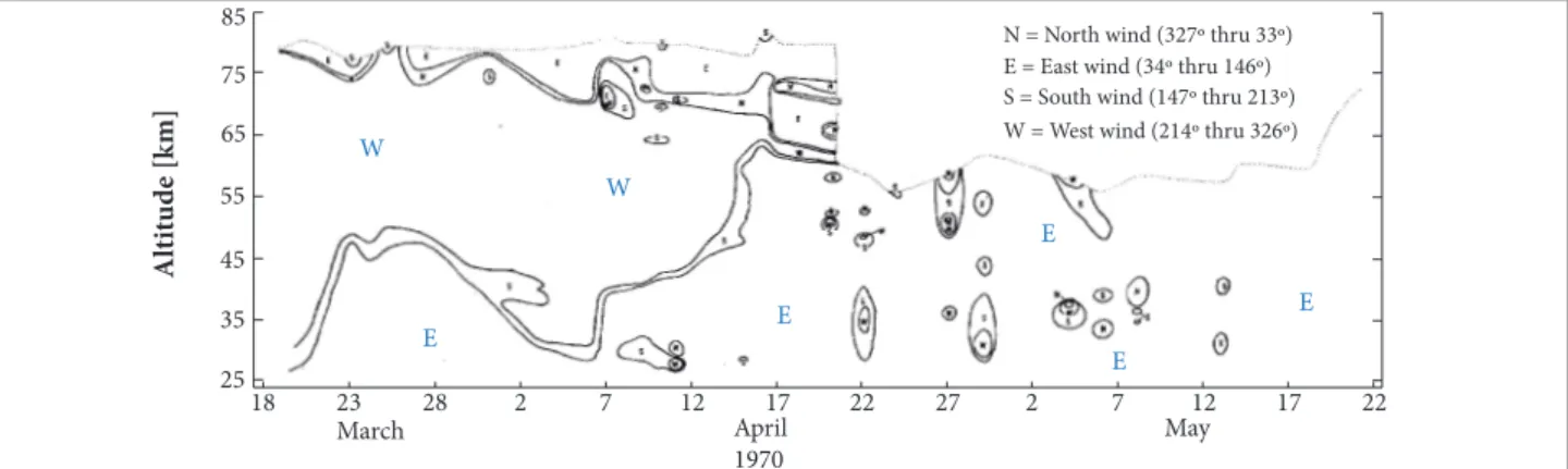
Figures 1 and 2 present the 16 wind-direction and speed proiles, respectively, from ~ 60 to 80 km altitude. he 2 wind igures plotted are from the tabular wind data which had been interpolated to the whole kilometer altitude levels. Data are also interpolated where there is no measured values. Wind directions are deined as follows: east winds are all those from 34° through 146°; south winds, from 147° through 213°; west winds, from 214° through 326°; and north winds, from 327° through 33°. Also shown are the conventional Loki-Dart meteorological rocket wind soundings which extends the Cajun-Dart primary data to lower altitude levels. he Loki-Darts were launched within 2 h of the Cajun-Darts. he ield project results indicated that the WW and SE extend at least up to 75 km altitude, with wind
Figure 1. Vertical time analyses — wind direction over NASA’s KSC. Plot of Cajun/Super Loki Dart and Loki Dart wind directions from late March through mid-May, 1970.
Al
ti
tu
d
e [k
m]
25 65 75 85
55
45
35
March April
1970
May
18 23 28 2 7 12 17 22 27 2 7 12 17 22
N = North wind (327º thru 33º) E = East wind (34º thru 146º) S = South wind (147º thru 213º) W = West wind (214º thru 326º)
W
W
E E
E E
directions somewhat erratic above this level. Webb (1964) and Mitchell (1970) have discussed the Continental wind regime changes that occur in the Spring and Fall in detail, so these dynamics will not be presented here.
Basic Wind Analysis
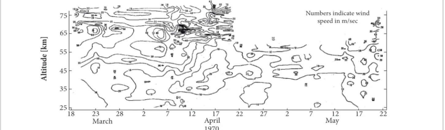
Webb (1964) indicates that the Stratospheric Circulation Index (SCI), at NASA’s KSC, shifts from a westerly winter component to an easterly summer wind component around the end of April at the 50 km altitude level. Figure 1 indicates a breakdown of the dominant winter westerly low starting around mid-April. In the 45 to 50 km region, for that day, the wind showed a southerly direction with future days exhibiting an easterly low pattern. he summer easterly regime began to dominate completely by the end of May 1970. he entire 25 through 80 km region wind directions given in Fig. 1 shows a general clockwise shiting of the wind with altitude. In the late winter regime easterly low prevailed below 35 km and shited through the south to the west throughout the 50 to 70 km region. From here it shited through north to another easterly regime above 70 km. Unfortunately, no high altitude wind data were taken ater April 20th, thereby leaving a void in the high altitude wind pattern during this transition period. Wind speeds during the winter regime, shown in Fig. 2, indicate a band of strong winds from 65 to 70 km altitude enveloped by weaker winds below and above. hese strong winds became less intense around April 15th as the winds turned easterly. Strong winds did exist between 70 and 80 km altitude just before and ater April 15th. he high winds speeds observed below 70 km altitude in Fig. 2 may be questionable, since wind data measured in this altitude region (by radar tracking of the chaf cloud) are usually unreliable because of chaf dispersion.
Overall, from February 1964 through April 1970, there were a total of 92 NASA wind rockets launched from KSC with 74 being successful. Looking at all months with data, the wind low data indicate a westerly wind low trend at most high altitudes (> 65 km) from November through March, with easterly winds prevailing from May through September. October and April appear to be the transitional wind shit months. he soundings indicate peak mesospheric wind speeds to be generally higher in winter (129 m/s) than in late summer (40 m/s). Mission planning could be afected by not considering that the Spring and Fall wind directional changeover when selecting a launch date or a re-entry date for a light. Engineering applications of wind and wind shear data from this high altitude region are principally concerned with design requirement regarding stage separation capability relative to ensuring adequate stage separation performance. See Turner et al. (1971) for all details,
data accuracy, the radar tracking errors, and overall conclusions.
THE NASA/MSFC ATMOSPHERIC VARIABILITY EXPERIMENT MEASUREMENT PROGRAM
NASA conducted a number of AVE throughout the 1970s, involving measuring the lower and upper atmosphere during the Great Plains Spring storm seasons. hese AVE ield projects were accomplished to better understand the dynamics of the lower atmosphere during storm events in order to enhance our knowledge of these phenomena and the applications that can be made toward development of atmospheric criteria used in support of launch/space vehicle lights near or through storm areas.
Two AVEs have been chosen here. he AVE-IV ield project of 1975 and the AVE-Severe Environmental Storms And Mesoscale Experiment (AVE-SESAME-1) ield project of 1979.
Figure 2. Vertical time analyses — wind speed (m/s) over NASA’s KSC. Plot of Cajun/Super Loki Dart and Loki Dart wind speeds from late March through mid-May, 1970.
Al
ti
tu
d
e [k
m]
25 65 75
55
45
35
March April
1970
May
18 23 28 2 7 12 17 22 27 2 7 12 17 22
hese 2 Great Plains measurement programs involved measuring the environment with both surface instrumentation and 3-h separation rawinsonde balloon measurements alot (42 U.S. stations east of the Rockies) during a severe weather outburst. Much analysis has been done on all the AVE data, but what is presented here, from Johnson (1982), is the stability analysis for AVE-IV data, in which a new stability index (Johnson Lag Index — JLI) was developed. his index was designed to forecast or give warning, in advance, of approaching severe weather (tornadoes). he JLI was then applied on a diferent and independent AVE-SESAME-1 measurement program in order to test this new index with 14 other standard and popular stability indices used in severe weather prediction. he 14 other stability indices used in this study were: SWEAT, Vertical Totals, Cross Totals, Total Totals, heta E (Ѳ
*
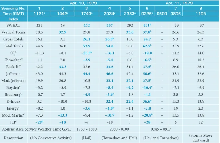
E), Showalter, Rackcliff, Jefferson, Mod. Jefferson, Boyden, Bradbury, K-Index, Energy, and Modiied Martin. Refer to NASA TP-2045 (Johnson 1982) for the deinition and details regarding all these stability indices. However, since the JLI was derived in order to forecast 3 to 6 h in advance of severeweather (typical of nowcasting), it was applied to the onslaught of severe weather observed at Abilene TX during AVE-SESAME-1. he JLI performed well in warning in advance of AVE-SESAME-1 severe weather, as shown in Table 1.
Stability Index Background
An investigation was made to determine whether the stability and vertical structure of an average “AVG” severe storm sounding, consisting of both thermodynamic and wind dynamical profiles, could be distinguished from an average “LAG” sounding taken 3 to 6 h prior to severe weather occurrence. he term “average” is deined here to indicate the arithmetic mean of a parameter, as a function of altitude, determined from a large number of available observations taken either close to the severe weather occurrence (AVG), or else more than 3 h before it occurs (LAG). he investigative computations were also accomplished to help determine if a severe storm forecast scheme or “index” could possibly be developed or efectively used.
Table 1. Abilene, Texas, AVE-SESAME-1 sounding stability index values during April 10 – 11, 1979.
aHighlighted values indicate the highest three unstable index values for each index;bMost unstable stability index value; cIndices in which instability is negative (–).
Apr. 10, 1979 Apr. 11, 1979
Sounding No. 1 2 3 4 5 6 7 8
Time (GMT) 1121a 1442a 1740a 2034a 2333a 0226a 0600 0806 1105
Index
SWEAT 221 69 472 557 292 621b – –33 –37
Vertical Totals 28.5 32.9 27.8 27.9 35.0 37.8b – 26.6 26.3
Cross Totals 16.1 3.1 26.1 26.9b 15.0 24.7 – 9.3 6.3
Total Totals 44.6 36.0 53.9 54.8 50.0 62.5b – 35.9 32.6
Ѳ* E
C –11.3 –8.1 –25.9b –16.1 –6.0 –12.0 – 11.2 14.0
ShowalterC –1.1 7.0 –3.9 –5.0 0.8 –6.5b – 8.9 10.3
Rackclif 32.2 33.3 32.6 33.6 31.4 37.5b – 26.0 26.1
Jeferson 43.0 44.3 44.4 46.6 42.4 50.6b – 33.1 32.6
Mod. Jeferson 19.9 20.8 10.5 33.4 27.1 37.5b – 21.9 22.9
BoydenC –3.2 –3.9 –7.3 –8.9 –9.2 –10.4b – –7.1 –6.9
BradburyC –0.7 1.7 –4.9 –5.6b –1.8 –4.1 – 2.8 3.8
K-Index 0.2 –10.0 –10.8 32.4 22.4 36.6b – 15.3 13.9
EnergyC –0.2 1.0 –3.6 –4.0b –1.1 –2.8 – 1.9 2.3
Mod. MartinC –7.3 –13.3 –9.4 –10.7 –1.2 –20.8b – 13.5 13.8
JLIC –29b –18 –7 –10 1 –28 – 6 12
Abilene Area Service Weather Time GMT 1730 – 1800 2050 - 0100 0245 – 0817
Description (No Convective Activity) (Hail) (Tornadoes and Hail) (Hail and Tornadoes) (Storms Move
he investigation presented these mean vertical proiles of thermodynamic and dynamic parameters as a function of severity of the weather, determined from manually digitized radar (MDR) categories observed during the NASA Atmospheric Variability Experiment IV (AVE-IV). he MDR “D” category represents the most severe radar storm category. Profile differences and stability index differences were computed along with the development of the JLI, which was determined entirely based on environmental vertical parameter diferences between conditions 3 h prior to severe weather and the severe weather itself. he JLI, along with 14 other stability indices, were then subsequently tested on a separate and independent data sample (AVE-SESAME-I) consisting of individual soundings taken during the April 10 – 11 1979 AVE-SESAME-I Project. he stability index computations were made on each of the AVE-SESAME-I data proiles.
Johnson Lag Index Development Details
A forecast-type procedure or index development was undertaken based entirely upon the differences noted in the averaged AVG and LAG meteorological proiles. If the environment 3 to 6 h prior to severe weather shows any type of parametric structure diferences from that at the time of severe weather, a stability index or procedure can be developed to model this phenomenon. Since wind diferences are small between LAG and AVG profiles, and the individual wind proiles are so variable, it was believed that for this initial index development attempt winds should not be used, but only the signiicant thermodynamic parameter changes versus altitude in order to keep the index simple.
he major diferences observed in the temperature structure between LAG and AVG proiles occur throughout the 800- to 650-hPa and the 650- to 500-hPa levels. he mainѲE diferences noted occurred between the 900- to 800-hPa and the 750- to 700-hPa levels. he LAG and AVG temperature and equivalent potential temperature lapse rates that exist between these pressure levels were then calculated. A gradient halfway between the LAG and AVG gradients was selected as being a most representative standard of atmospheric conditions between 3 h prior to storms and storm occurrence itself. Lapse rates on one side of this standard gradient would represent conditions of the LAG, while gradients observed on the other side of this standard would represent AVG conditions. Four thermodynamic terms were selected as potential forecast terms: 2 terms to represent temperature gradients in lower and upper atmospheric areas
and 2 ѲE gradient terms to represent the low- and middle-atmosphere temperature and moisture structure. he 4 terms were then combined so as to maximize the negative value of the index in representing extreme instability only during LAG-D time (3 to 6 h before storms). Since this gradient procedure, or index, is maximized a few hours before storm occurrence, the application of the index during periods of severe weather (AVG-D conditions) should result in a positive value. his JLI is expressed as:
where: T
650 − 800= T650 − T800; T500 − 650 = T500 − T650 ,
ѲE 800 − 900= ѲE 800 − ѲE 900; ѲE 700 − 750= ѲE 700− ѲE750 (T and
ѲE units in °C or K).
he 4 terms of Eq. 1 were weighted by applying multiplication factors of 1, 2, 2, and 1/3, respectively. his was done to ofset the efect of the category A (non-precipitation) small temperature and potential temperature gradients, which tended to allow the un-weighted JLI equation to produce an unstable negative JLI value close in magnitude to LAG-D JLI conditions. hus, this weighting will help eliminate the occurrence of false alarms whenever category A, non-precipitation areas are encountered. The weighting factors were determined from a subjective, trial-and-error procedure involving diferent combinations of weighting, in order to arrive at a large JLI diference between category A (non-precipitation) and D (severe storm) conditions. he JLI values calculated for LAG-D conditions equaled −4.35 dimensionless. Likewise, JLI values computed for AVG-D conditions resulted in a value of +2.76 dimensionless. he theory, then, is that if atmospheric conditions from an individual sounding produce a negative JLI of similar or greater magnitude, one should expect severe weather to occur within the next three to six hours. his theory will be tested as to its performance along with the other stability indices. he question is: how well will the JLI model the real atmosphere?
Stability Index Comparison During the Similar AVE-Sesame-I Environment
Since stability is the item of interest in the present in- vestigation, the 15 stability indices mentioned earlier were computed for each AVE-SESAME-I Abilene TX soundings. hese stability index results are presented in Table 1, together with the exact time of radiosonde release. Listed below the
(1)
JLI = (−11.5 − Δ
T
650 − 800) + 2(Δ
T
500 − 650+ 14.9) +
index values in this table is a severe weather timeline applicable to the north-central Texas area, within 150 mi of Abilene. Also on Table 1, the highest 3 unstable index values for each index have been highlighted in blue for easy reference. he most unstable value has also been marked with a superscript “a”. As can be seen in Table 1, there seems to be good general agreement that most all indices appear to perform adequately in the evaluation of atmospheric instability during the passage of the 2 squall systems near Abilene. Proiles 4 and 6 were the 2 soundings taken at Abilene just prior to the severe weather which occurred near and around the city. Stability index values from Table 1 indicate that most indices peak (with instability) using soundings 4 and 6 data, 10 of the 15 indices peak using sounding 6, while 3 peak using sounding 4. his means that 13 of the 15 peaked during the occurrence of upper-level moisture buildup, just prior to the onset of the Abilene storms. Only 2 indices (Ѳ*E and JLI) peaked at times prior to this. Sounding 6
is more unstable than sounding 4 because the storms developed very close to the sounding site, and the moisture alot had developed more extensively than during sounding 4. he dry-line passage at Abilene between 2200-0000 GMT can readily be seen by the sudden increase in stability in most all of the indices during sounding 5 (2333 GMT). While weather activity existed eastward of Abilene during sounding 8 (0806 GMT, April 11), all indices show a general increase in stability as the cold front arrives. Table 1 also hints that soundings taken when storms are not in progress in the general area result in slightly greater instability than when storms have formed in the area during the radiosonde release. his may seem to indicate that the instability (stored potential energy) which can build up prior to storm occurrence can be relieved (made more stable) through the release of thunderstorm kinetic energy activity.
Lag Testing
It was indicated that, based on the AVE-IV LAG proile as it related to the AVG proile, 3 indices appeared to be potential lag indices. hese indices were: SWEAT, Modiied Martin, and the JLI. According to the AVE-SESAME-I sounding data (Table 1), all of these indices, with the exception of the JLI, fail to qualify as a lag index, since the peak index outliers which occur before storm development have been explained away. he JLI does give large negative values (−29 and −18) during the non-storm time period represented by soundings 1 and 2. When distant storms occur, Abilene sounding 3 records a JLI = −7. Just prior to the irst major outbreak of storms closer
to Abilene, sounding 4 gives a JLI = −10. he dry-line passage, during sounding 5, produces a JLI = +l. Sounding 6, released 19 min prior to hail occurrence near Abilene (51 min prior to irst tornado report), gave a JLI = −28. his large negative index value was surprising, since the sounding represents squall line-produced activity. However, the JLI could still be sensing the intense, unstable, pre-squall line environment which appears not to have passed the balloon release site at this time. Overall, the JLI has functioned well and it gives large positive values (+6 and +12) when the cold front moved into the area. his indicates that perhaps no more storms were due to follow. Based on this one severe storm case, it appears that, of 15 stability indices tested as a pre-storm lag (3 to 6 h prior) forecast index, only the JLI appears to give satisfactory results thus far.
he JLI stability index was developed from AVE-IV (1975) soundings and then tested on AVE-SESAME-1 (1979) soundings. However, since the JLI is a new index, representing low- and middle-level temperature and moisture, it will have to be tested further and possibly be adjusted, before it can quality as a lag/forecast index for only severe Great Plains storms. his stability study indicates that these ield program empirical data can indeed be used for atmospheric disciplinary research in order to better understand the severe storm environment that can afect launch and space vehicle travel near or through it.
NASA/MSFC SEQUENTIAL HIGH RESOLUTION JIMSPHERE WIND PROFILE MEASUREMENT PROGRAM
the behavior and generating mechanisms of mesoscale wind proile luctuations.
Acquisition of high-resolution or detailed wind proile measurements within the troposphere and lower stratosphere has been possible by the use of a specially designed constant-volume aluminized mylar balloon tracked by a high-precision radar (MP16). he constant-volume balloon (or Jimsphere-radar system) has been utilized to acquire a very unique set of wind proile measurements. his system is capable of providing resolution of 50 to 100 m wavelengths for the altitude region from approximately 200 m to 18 km.
his measurement program and its engineering application to the launch and the design of aerospace vehicles is the subject of this paper’s section. he various, detailed changing wind characteristics of these wind data sets can be obtained from Johnson and Vaughan (1978) and Vaughan (1977), which give a complete description and information concerning the system and the entire data bases. Harrington (2011), along with Blair et al. (2011, 2001), give detailed information as to
the application of the sequential Jimsphere measured wind proiles for design and launch. Much from Harrington (2011) is presented in this section.
he sequential data sets consist of 3 or more Jimsphere-radar wind proile measurements made over a period of hours (varying from approximately 6 to 24 h) with time separations from 1.5 to approximately 3 h. Horizontal wind speed and direction at 25 m height intervals from near the surface to approximately 18 km altitude were acquired as reported in Johnson and Vaughan (1978). he data is directed to 2 diferent groups of investigators: those involved in “engineering” studies concerning the design and launch of aerospace vehicles (rockets, space vehicles, and aircrat) and those involved in “disciplinary” studies concerning the mesoscale dynamic characteristics of the wind low in the troposphere and lower stratosphere. Engineering applications will mainly be presented here.
Engineering Applications
he original and current use for which these data were acquired is to provide important inputs in the aerospace vehicle engineering area. All near vertically rising vehicles have one point in common: the susceptibility or vulnerability of their structural and control systems to the wind proile characteristics through which they must perform. herefore, their performance under operational conditions is directly proportional to the design ability of the launch/space vehicle systems relative to
the wind characteristics measured and speciied for the vehicle development.
Data Description
he reader should be referred to the Johnson and Vaughan (1978) and Vaughan (1977) references in order to get a complete description and analyses of all the various short- and long-term wind characteristics that are evident from these sequential series. Only some general measured wind proile information will be given here. he most signiicant features of the wind proile are wind speed and direction luctuations which persist, oten throughout the whole series, at approximately the same altitude. Speciically, the following categories of wind speed perturbations may be recognized:
• Large-scale (jet stream) perturbations having a vertical wavelength generally greater than approximately 5 km and an amplitude greater than 20 m/s and usually persisting unchanged throughout the series.
• Mesoscale perturbations having a vertical wavelength from approximately 0.2 to 2 km and an amplitude up to approximately 15 m/s. Individual wind speed maximums from these perturbations persist from several hours to a time period longer than that over which the sequential measurements were taken. Oten the amplitude and occasionally the vertical wavelength of the perturbations change considerably from one proile to the next so that successive perturbations are not exact replicas of each other yet can still be identiied as the same feature rather easily.
• Small-scale (turbulence) perturbations having a vertical wavelength less than approximately 500 m and an amplitude up to approximately 6 m/s. hese oscillations difer from the small mesoscale features principally because of their highly transient nature. They are common perturbations on a given proile but lack continuity in time.
Figure 3. (a) Example of jet stream winds; (b) Example of sine wave l ow in the 10 to 14 km altitude region; (c) Example of high wind speeds over a deep altitude layer and (d) Example of low wind speeds
Al ti tu d e [k m]
Wind speed [m · s-1] Wind speed [m · s-1] Wind speed [m · s-1] Wind speed [m · s-1]
4,000 2,000
0 10 20 30 40 50 60 70 80 0 10 20 30 40 50 60 70 80 6,000 8,000 10,000 12,000 14,000 16,000 18,000 20,000 4,000 2,000 6,000 8,000 10,000 12,000 14,000 16,000 18,000 20,000 4,000 2,000 6,000 8,000 10,000 12,000 14,000 16,000 18,000 20,000 4,000 2,000 6,000 8,000 10,000 12,000 14,000 16,000 18,000 20,000
0 10 20 30 40 50 60 70 80 0 10 20 30 40 50 60 70 80
Al ti tu d e [k m]
Scalar wind speed [m · s-1] 4,000
2,000
0
0 10 20 30 40 50 0 10 20 30 40 50 6,000 8,000 10,000 12,000 14,000 16,000 18,000 4,000 2,000 0 6,000 8,000 10,000 12,000 14,000 16,000 18,000
Figure 4. Examples of discrete gusts.
Al ti tu d e [k m]
Wind speed [m · s-1] 0 0.0 2.5 5.0 7.5 10.0 12.5 15.0 17.5
20.0 4–5 July 1966
a.
2321GMT 0040 0245 0516 0730 0930
b. c. d. e. f.
g. Average
10 20 0 10 20 0 10 20 0 10 20
Figure 5. Sequential wind speed proi les measured at Cape Kennedy, July 4 – 5, 1966.
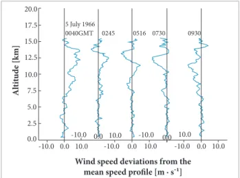
These wind features can be visualized in Figs. 3 through 4. Figures 5 and 6 give an example of a set of sequential Jimsphere wind profile speed measurements taken at Cape Kennedy, Florida, on July 4 – 5, 1966. The average of the 6 vertical profiles is given in the right of Fig. 5. The deviations of the individual profiles from the average profile are presented in Fig. 6. The changes in wind speed between the profiles can also be calculated. Studies like this utilizing many Jimsphere sequences can help determine the structure and the changing structure type statistics that can be used as inputs in engineering vehicle design and development and in applying limits in the day-of-launch (DOL) countdown timeframe. Al ti tu d e [k m]
Wind speed deviations from the mean speed profile [m · s-1] 0.0 0.0 0.0 0.0 0.0 0.0 -10.0 -10.0 -10.0 -10.0 -10.0 10.0 10.0
5 July 1966
0040GMT 0245 0516 0730 0930
10.0 10.0 10.0 2.5 5.0 7.5 10.0 12.5 15.0 17.5 20.0
Figure 6. Cape Kennedy July 5, 1966 deviations of individual wind speed proi les from the average proi le.
DISCUSSION
The various features of the wind profiles and their behavior as a function of time and altitude are of considerable importance in the design and operation of aerospace vehicles. The influence of low frequency or mean wind profile features can often be accommodated by DOL wind biasing or trajectory shaping techniques. This could eliminate a considerable portion of the forcing function created on the structural and control system due to this category of wind speed perturbation where demanded by a particular vehicle’s development limitations and operational requirements. However, other categories of the wind profile perturbations must be accounted for within the design of the vehicle system or avoided if possible during launch operations. There is no way to avoid the small-scale or turbulent category of the wind profile; therefore, it must be incorporated into the design capability at a minimum risk level and allowed for in any pre-launch monitorship simulation since it cannot be predicted in a deterministic manner for expected launch in-flight winds. This leaves the mesoscale category of wind profile features that contains the frequencies of most concern to structural and control system responses.
JIMSPHERE BALLOON DOL APPLICATION
Much of the following is taken from Harrington (2011). Blair et al. (2001, 2011) give further details of how the Jimsphere
balloon wind data is inputted/applied during DOL countdown.
Trajectory Design
To minimize vehicle loads while maximizing vehicle performance, a DOL trajectory must be designed and veriied for the vehicle’s safety. he DOLtrajectory is tailored to the speciicwind and atmospheric conditions on the launch day, which increases the probability of launch.
A multitude of vehicle responses are affected by the forces produced as a result of the wind profile characteristics. These are especially critical during the higher dynamic pressure portion of the flight path or trajectory. Furthermore, these responses are a function of trajectory shaping, control system gains, structural damping, vehicle configuration, operational characteristics, etc. The sequential Jimsphere wind samples provide information on the short term (few hours) variability in wind profiles. This information was used by the NASA Shuttle Launch System Evaluation Advisory
Team (LSEAT) relative to go/no-go recommendations hours prior to L-0. It provided inputs for the delta wind loads versus time for use during the pre-launch wind load
calculations.
Day-of-Launch I-Load Update Process Used
The Day-of-Launch I-Load Update (DOLILU) is the process by which NASA’s Space Shuttle Program tailored the vehicle steering and throttle commands to fit that day’s environmental conditions and then rigorously verifies the integrated vehicle trajectory’s loads, controls, and performance. The Space Shuttle DOLILU system requires wind speed, wind direction, and atmospheric thermodynamic data measured on the DOL. This DOL wind biasing approach tends to reduce loads without a large impact to vehicle performance capability. Weather balloon data (Jimsphere and Automated Meteorological Profiling System (AMPS)/Radiosonde) measured at NASA’s KSC launch site is transmitted to NASA’s Marshall and Johnson Space Centers. Jimsphere balloon data are then used as an input to design of the first stage guidance parameters or initialization loads (I-load). The vehicle will experience the highest dynamic pressure (Qbar) near 35,000 ft. Launch day winds will have an impact on the sensed loading which will tend to pull the trajectory away from the desired staging targets. The resulting trajectory prediction is assessed to verify that all trajectory, control, systems, structural loadin, and performance constraints are met. Additionally, these assessments statistically protect for non-observed dispersions. One such dispersion is the change in the wind from the last measured Jimsphere balloon to launch time. This Jimsphere measurement process is started many hours before launch and is repeated several times as the launch count proceeds. About 2 h before lift-off, the DOL trajectory design is frozen and I-loads are uplinked to the Space Shuttle. Additional constraint verification assessments are completed using the Jimsphere balloon wind measurements made closer to launch. If the final constraint assessment results in a predicted constraint violation, based on the DOL trajectory design and latest Jimsphere balloon measured winds, then the launch is scrubbed.
Day-of-Launch Timeline
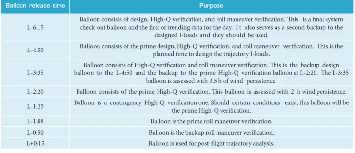
anticipate whether large changes in the wind might be probable throughout the day of launch countdown. Low-Resolution radiosonde balloons that DOLILU uses for atmospheric thermodynamic data are released at L-9:00; L-6:20; L-3:45; and L-0:30. For wind data, Jimsphere balloon release times are: L-6:15; L-4:50; L-3:35; L-2:20; L-1:25; L-1:08; L-0:50 and one post-light at L+0:15. he inal DOLILU go/no-go is given at L-0:30. While the DOLILU process is basically repeated, each Jimsphere balloon wind proile assessment has diferent purposes as Table 2 shows.
he designed trajectory is optimized (biased) for a speciic wind, but has been demonstrated to be valid for the actual launch wind. In operations, the nominal design balloon is released at L-4:50, with the irst backup at L-3:35. he I-load balloon is chosen based on visual comparison from the L-4:50 balloon to the forecast one. Should a large amount of change be observed or predicted, the timeline will support a delay in the design of I-loads until the L-3:35 balloon. he updated I-load tables are uplinked to the Orbiter on the launch pad at roughly 90 min before launch. Constraint assessments are required to be made using later balloon measurement in order to account for wind changes which may adversely impact vehicle constraints.
Trajectory Design Details
For trajectory design, DOLILU designs the pitch, yaw, and throttle commands for the Space Shuttle. he DOLILU design targets an optimal angle-of-attack (α) schedule to −4°, which reduces wing loading during ascent, targets angle-of-sideslip (β) to 0° to reduce side loads, and recalculates the throttle
Balloon release time Purpose
L-6:15
Balloon consists of design, High-Q veriication, and roll maneuver veriication. his is a inal system check-out balloon and the irst of trending data for the day. I t also serves as a second backup to the
designed I-loads and they should be used.
L-4:50 Balloon consists of the prime design, High-Q veriication, and roll maneuver veriication. his is the
planned time to design the trajectory I-loads.
L-3:35
Balloon consists of High-Q veriication and roll maneuver veriication. his is the backup design balloon to the L-4:50 and the backup to the prime High-Q veriication balloon at L-2:20. he L-3:35
balloon is assessed with 3.5 h of wind persistence.
L-2:20 Balloon consists of the prime High-Q veriication. his balloon is assessed with 2 h wind persistence.
L-1:25 Balloon is a contingency High-Q veriication one. Should certain conditions exist, this balloon will be
the prime High-Q veriication.
L-1:08 Balloon is the prime roll maneuver veriication.
L-0:50 Balloon is the backup roll maneuver veriication.
L+0:15 Balloon is used for post-light trajectory analysis.
Table 2. DOLILU balloon purposes.
command to keep the maximum dynamic pressure (Qbar) near a design target. DOLILU rebalances the steering and throttle command tables.
Structural Load Indicator Constraints
Airloads and throttle-sensitive structural loads certiication constraints are evaluated on DOL to verify that the predicted trajectory is within certiication. Simpliied structural load indicators (SLI) were developed to determine element structural loadings given a newly designed trajectory on DOL. Forty-two SLI protect speciic points on the integrated vehicle, such as Shuttle to ET attach loads.
Parameter Constraints are also applied during countdown. There is also Wind Persistence Dispersion procedures that are applied using Jimsphere wind profile pairs.
Wind Persistence Dispersion
The DOLILU system will give the final trajectory assessment based on the L-2:20 balloon data. This is the final go/no-go placard due to the 65-min balloon rise, computer processing time, quality assurance, and reporting time. Therefore, the final DOLILU assessment does not truly assess the real wind that the Space Shuttle will experience. The wind from the surface to 60,000 ft will continue to change through to launch time and the impact on any actual constraint may not be completely understood without a full assessment. “Wind persistence” is the term given to define this lack of temporal persistence on the vehicle constraints due to the changing wind. To develop the wind persistence dispersion, NASA’s Space Shuttle Program utilized a database of previously measured Jimsphere wind profiles measured from the launch site at fixed intervals. Wind profiles measured at about 2 and 3.5 h apart were cataloged and totaled 1,000 wind profile pairs. This database is further split into seasons and analyzed independently. For the first of the wind pair, a trajectory design was generated, the trajectory was flown, and the Q-plane’s α, βminimum margin was determined. For the second of the pair, the design was from the first wind was flown through using the second wind and the Q-Plane α, βMinimum Margin was determined. Using this minimum margin data, the mean and standard deviation of the first of the pairs and of the second of the pairs can be computed. Additionally, the correlation coefficient between each can be computed. This data will be used in a bivariate conditional Gumbel probability distribution. Only 2 dispersion increments were developed: 2 and 3½ h. Therefore, inside of 2 h to launch, the 2-h increment is utilized. Should the contingent L-1:25 hour Jimsphere balloon wind assessment be required, the result might be slightly conservative. However, closer to launch, there exist other means to protect the DOLILU design with wind-only assessments, by the MSFC Environments Team who monitor, examine, and evaluate the various DOL wind data for any evidence of sudden wind changes.Vehicle Certification and Launch Probability
For vehicle certification, the final launch probability is a quasi-Monte Carlo process where various DOL winds and atmospheric data are entered into the DOLILU design and assessment process to report a go percentage. A winds database of 150 measured Jimsphere balloons for each month is combined with monthly measured atmosphere (thermodynamic) data. DOLILU then uses each wind and atmosphere measurement for design and constraint assessment. This results in 150 go or no-go placards. Thus, the percent go is probability of launch.
SEQUENTIAL JIMSPHERE WIND MEASUREMENT CONCLUSIONS
The intent of this section on “Jimsphere Balloon DOL Applications” has been to provide the engineering (and the disciplinary) oriented reader with a better insight into the behavior of the mesoscale wind flow in the troposphere and lower stratosphere as it applies to the design and to the launch of space vehicles. DOLILU has significantly improved launch probability over other design methodologies. If DOLILU did not exist, and a mean wind design was utilized for the Space Shuttle, the launch probability for February would be reduced from about 90% to about 30%. This is the effectiveness of DOLILU, which re-centers and reduces the vehicle loads, while normalizing ascent performance. Thus, the Jimsphere profiles taken on DOL and those Jimsphere profile sequential data sets archived in 1,000 Seasonal Pairs or in 150 monthly profiles all help in vehicle launch success.
Keep in mind that for a successful launch of the Space Shuttle not only the Sequential Jimsphere measured winds are used, but also many other NE Weather Launch Commit Criteria need to be followed and met for both launch and landing success. See Diller (2003).
SUMMARY REMARKS
measurement program may be the answer in supplying this needed data.
In summary, some of the key beneits for launch/space vehicle development achieved from the acquisition of the data provided by these 3 unique specialized ield programs include the following programs/experiments.
METEOROLOGICAL ROCKET WIND MEASUREMENT PROGRAM
Knowledge concerning the magnitude of mesospheric wind velocity, direction and associated wind shears at altitudes above those achieved by rawinsonde balloon measurement (~ 30 km) is needed for the design of launch/ space vehicle control capability and stage separation for the KSC launch site. The measurements of these wind profile conditions were provided by high-altitude meteorological rockets typically measuring winds in the 60 to 85 km region. Thermodynamic conditions can also be measured by other rocketsondes and applied in the development of reference atmosphere models used in launch/space vehicle trajectory, engineering calculations, etc.
ATMOSPHERIC VARIABILITY EXPERIMENTS Knowledge of the tropospheric atmospheric variability (time and space) over varying periods was of particular benefit regarding the planning of vehicle launches and operations, as well as in the forecast of severe un-stable weather for an area in which the vehicle’s trajectory may travel through
on launch or during re-entry for southern United States and KSC launch site. The AVE field experiments provided this information for use in weather forecast developments relative to launch/space support operations.
SEQUENTIAL HIGH RESOLUTION JIMSPHERE WIND PROFILE MEASUREMENT PROGRAM
Knowledge of the detail characteristics of tropospheric wind proiles over aerospace vehicle launch sites is of particular value for establishing in particular the structural design characteristics, in addition to control system requirements associated with the maximum dynamic pressure region of the launch/space vehicle light. he beneit of the Jimsphere Wind Proile Measurement Program at the KSC launch site provided information on the variability of the detail wind characteristics associated with the pre-launch monitorship of structural loading of a launch/space vehicle, thereby enabling allowances to be made as function of time for the pre-launch simulation of launch/space structural loads and control system performance.
AUTHOR’S CONTRIBUTION
Johnson DL conceived the idea.Vaughan WW and Johnson DL co-wrote the text based on the contributions of various research programs from selected NASA natural environment ield projects and applications for launch vehicle development.
REFERENCES
Blair JC, Ryan RS, Schutzenhofer LA (2011) Lessons learned in engineering. NASA/CR— 2011–216468; [accessed 2016 Sept 30]. http://www.vibrationdata.com/NASA_CR_2011_216468.pdf
Blair JC, Ryan RS, Schutzenhofer LA, Humphries WR (2001) Launch vehicle design process: characterization, technical integration, and lessons learned. NASA/TP--2001-210992; [accessed 2016 Sept 30]. http://ntrs.nasa.gov/archive/nasa/casi.ntrs.nasa. gov/20010066713.pdf
Diller G (2003) Space shuttle weather launch commit criteria and KSC end of mission weather landing criteria. KSC release 13-03; [accessed 2016 May 03]. http://www.nasa.gov/centers/kennedy/ news/releases/2003/release- 20030128.html#.V4_PhKXEqOs. email
Harrington BE (2011) Space shuttle day-of-launch trajectory design operations. JSC-CN-22667, JSC-CN-24595, JSC-CN-24725. Proceedings of the AIAA Space 2011 Conference; Long Beach, USA.
Johnson DL (1982) A stability analysis of AVE-IV severe weather soundings. NASA TP-2045; [accessed 2016 Sept 30]. http://ntrs. nasa.gov/archive/nasa/casi.ntrs.nasa.gov/19830006553.pdf
Johnson DL, editor (2008) Terrestrial environment (climatic) criteria guidelines for use in aerospace vehicle development, 2008 revision. NASA/2008-215633; [accessed 2016 Sept 30]. http://ntrs.nasa. gov/archive/nasa/casi.ntrs.nasa.gov/20090022159.pdf
Johnson DL, Vaughan WW (1978) Sequential high-resolution wind proile measurements. NASA TP-1354; [accessed 2016 Sept 30]. http://ntrs.nasa.gov/archive/nasa/casi.ntrs.nasa. gov/19790006509.pdf
Mitchell LV (1970) Variability of the monthly mean zonal wind, 30-60 km. Scott AFB, IL: AWS. Technical Report No. 195.
nasa.gov/archive/nasa/casi.ntrs.nasa.gov/19710014563.pdf
Vaughan WW (1977) An investigation of the temporal character of
mesoscale perturbation in the troposphere and stratosphere. NASA
TN D-8445; [accessed 2016 Sept 30]. http://ntrs.nasa.gov/
archive/nasa/casi.ntrs.nasa.gov/19770011717.pdf