Claudio Ruggieri
[email protected] University of São Paulo Dept. of Naval Arch. and Ocean Engineering
J. of the Braz. Soc. of Mech. Sci. & Eng. Copyright © 2010 by ABCM October-December 2010, Vol. XXXII, No. 4 / 475 PNV – EPUSP
05508-030 São Paulo, SP, Brazil
A Micromechanics Approach to
Assess Effects of Constraint on
Cleavage Fracture Toughness: a
Weibull Stress Model
This work describes an engineering methodology incorporating the statistics of microcracks and a probability distribution of the (local) fracture stress to assess the effects of constraint loss and weld strength mismatch on crack-tip driving forces. One purpose of this investigation is to establish a definite fracture assessment framework capable of providing robust correlations between toughness data measured using small, laboratory specimens to large, complex structural components with varying crack configurations and loading modes (tension vs. bending). Another purpose is to verify the effectiveness of the proposed methodology building upon a local fracture parameter, here characterized by the Weibull stress, in structural integrity assessments of cracked components including steel weldments. Overall, the exploratory applications conducted here lend strong support to use Weibull stress based procedures in defect assessments of cracked structures.
Keywords: cleavage fracture, local approach, Weibull stress, constraint effect, weld strength mismatch
Introduction
1The fundamental importance of cleavage fracture behavior in
structural integrity assessments has stimulated a rapidly increasing amount of research on predictive methodologies for quantifying the impact of defects in load-bearing materials such as, for example, cracks in critical weldments of high pressure vessels. Such methodologies play a key role in repair decisions and life-extension programs for in-service structures (e.g., aerospace, nuclear and offshore structures) while, at the same time, ensuring acceptable safety levels during normal operation. For ferritic materials at temperatures in the ductile-to-brittle transition (DBT) region, fracture by transgranular cleavage along well defined, low index crystallographic planes (see, e.g., Averbach, 1965 and Tetelman and McEvily, 1967) is the dominant operative micromechanism. This failure mode potentially limits the load bearing capacity of the structure as local crack-tip instability may trigger catastrophic failure at low applied stresses with little plastic deformation.
Conventional methods of fracture mechanics analysis employ a one-parameter characterization of loading and toughness, most commonly the J-integral or the corresponding value of the Crack Tip Opening Displacement (CTOD, δ). The approach correlates unstable crack propagation in different cracked bodies based on the similarity of their respective near-tip stress and strain fields provided small scale yielding (SSY) conditions prevail. Under these conditions, near-tip plastic deformation is well-contained with plastic zones vanishingly small compared to the relevant physical dimensions in fracture specimens and structural components such as crack length, remaining ligament, etc. (see, e.g., the review by Hutchinson, 1983). However, the stress histories that develop in the near-tip region of a macroscopic crack in engineering structures containing shallow cracks are more often of different character than those for the high constraint SSY condition. At increasing levels of loading and deformation, large scale yielding conditions (LSY) gradually develop at the crack tip region, which relax the near-tip stress fields below the SSY levels, particularly for moderate-to-low hardening materials. The decreased level of crack-tip constraint and the strong interaction of remote loading with near-tip plasticity potentially cause significant elevations (factors exceeding 3~5) in
Paper accepted June, 2010. Technical Editor: Nestor A. Zouain Pereira.
the elastic-plastic fracture toughness for shallow crack configurations of ferritic steels tested in the transition region, where transgranular cleavage triggers macroscopic fracture. The enormous practical implications of this apparent increased toughness of common ferritic steels in low-constraint conditions, particularly in defect assessment and repair decisions of in-service structures, have spurred a flurry of new analytical, computational and experimental research over the past years.
More recent efforts within the framework of continuum fracture mechanics have focused on the development of two-parameter fracture methodologies to describe the full range of Mode I, elastic-plastic crack-tip fields with varying near-tip stress triaxiality. Within these methodologies, J sets the size scale over which large stresses and strains develop, while the second parameter, such as the T stress (Al-Ani and Hancock, 1991; Betegon and Hancock, 1991; Du and Hancock, 1991; Parks, 1992) or the nondimensional Q parameter (O'Dowd and Shih, 1991, 1992), scales the near-tip stress distribution. The approach also enables the introduction of a toughness locus for a specific material and temperature in connection with a J-Q driving force trajectory for each crack geometry; here, the toughness locus for the material is constructed upon determining the Q-value at fracture which corresponds to each measured -value (O'Dowd and Shih, 1991, 1992). However, the large number of fracture specimens and different temperatures needed to construct the J-Q toughness locus greatly complicate direct implementation of this approach to fracture assessments as does the application of the method (which derives from a 2-D framework) to fully 3-D crack geometries. Moreover, such models do not address the strong sensitivity of cleavage fracture to material characteristics at the microlevel nor do they provide a means to predict the effects of constraint and prior ductile tearing on toughness. In particular, the random inhomogeneity in local features of the material causes large scatter in experimentally measured values of fracture toughness ( , or CTOD). Such features do assessments of structural integrity using laboratory testing of standard specimens and simplified crack configurations to a complex task: what is the “actual" material toughness and how is the scatter in measured values of fracture toughness incorporated in defect assessment procedures?
c J
The above arguments that continuum fracture mechanics approaches do not suffice to characterize the fracture behavior of fully yielded crack geometries motivated the development of micromechanics models based upon a probabilistic interpretation of the fracture process (most often referred to as local approaches). Attention has been primarily focused on probabilistic models incorporating weakest link statistics to describe material failure caused by transgranular cleavage. In the context of probabilistic fracture mechanics, a limiting distribution describes the coupling of the (local) fracture stress with remote loading (as measured by J or CTOD). A fracture parameter associated with this limiting distribution conveniently characterizes macroscopic fracture behavior for a wide range of loading conditions and crack configurations. Batdorf and Crose (1974), Evans (1978) and Matsuo (1981) first considered models of this type to describe brittle fracture for arbitrary loading. Here, a convenient function describing the number of microcracks per unit volume failing at each value of the local tensile stress is used to arrive at the probability of fracture for a cracked body. Later, Beremin (1983), Wallin et al. (1984a, 1984b, 1986, 1993), Lin et al. (1986), Godse and Gurland (1989), Brückner et al. (1990), among others provided a link between the size of carbide particles dispersed in the material and the inhomogeneous stress fields ahead of a macroscopic crack. They sought to predict the dependence of fracture toughness ( ) on material properties and temperature.
Ic K
Among these earlier research efforts, the work of Beremin (1983) provides the basis for establishing a relationship between the microregime of fracture and macroscopic crack driving forces (such as the J-integral) by introducing the Weibull stress (σw) as a probabilistic fracture parameter. A key feature of the Beremin approach is that σw follows a two-parameter Weibull distribution (Weibull, 1951; Mann et al., 1974) in terms of the Weibull modulus, m, and the scale parameter, . Further idealization postulates that parameter m represents a material property in this model (Mudry, 1987) possibly dependent on temperature but invariant of loading history, which provides a means to correlate fracture toughness for varying crack configurations under different loading conditions. When implemented in a finite element code, the Beremin model predicts the evolution of the Weibull stress with applied load to define conditions leading to (local) material failure. Previous research efforts to develop a transferability model to elastic-plastic fracture toughness values rely on the notion of the Weibull stress as a crack-tip driving force (Ruggieri and Dodds, 1996a, 1996b; Ruggieri, 2001a, 2001b). The central feature in this methodology adopts the simple axiom that unstable crack propagation (cleavage) occurs at a critical value of the Weibull stress; under increased remote loading (as measured by J), differences in evolution of the Weibull stress reflect the potentially strong variations of near-tip stress fields and crack-tip constraint.
u
σ
This work describes an engineering methodology incorporating the statistics of microcracks and a probability distribution of the (local) fracture stress to assess the effects of constraint loss and weld strength mismatch on crack-tip driving forces. One purpose of this investigation is to establish a definite fracture assessment framework capable of providing robust correlations between toughness data measured using small, laboratory specimens to large, complex structural components with varying crack configurations and loading modes (tension vs. bending). Another purpose is to verify the effectiveness of the proposed methodology building upon a local fracture parameter, here characterized by the Weibull stress ( ), in structural integrity assessments of cracked components including steel weldments. Overall, the exploratory applications conducted here lend strong support to use Weibull stress based procedures in defect assessments of cracked structures.
w
σ
Probabilistic Modeling of Cleavage Fracture
Description of Scatter in Fracture Toughness Values
Fracture testing of ferritic steels in the DBT region consistently reveal large scatter in the measured values of cleavage fracture toughness. It is now widely known that such scatter in toughness data is essentially associated with the random location and orientation of fracture-triggering microcracks near the (macroscopic) crack tip (Anderson, 2005). The connection between the local (cleavage) fracture process and extreme value statistics plays the key role in describing the scatter in fracture toughness values. A continuous probability function derived from weakest link statistics conveniently characterizes the distribution of toughness values, Jc, in the form (Weibull, 1951; Mann et al., 1974).
( )
⎥⎥⎦ ⎤ ⎢
⎢ ⎣ ⎡
⎟⎟ ⎠ ⎞ ⎜⎜
⎝ ⎛
− − − − =
α
th th c c
J J
J J J
F
0
exp
1
(1)
which is a three-parameter Weibull distribution with parameters
(
α,J0,Jth)
. Here, α denotes the Weibull modulus (shapeparameter), defines the characteristic toughness (scale parameter) and is the threshold fracture toughness. In particular, parameter
0 J
th J
α represents a measure of the scatter in the toughness data; the larger this value, the less scattered is the toughness distribution (Mann et al., 1974).
The threshold fracture toughness is often set equal to zero, so that the Weibull function given by Eq. (1) assumes its more familiar two-parameter form in terms of parameters
0
=
th J
(
α,J0)
as( )
1 exp .0 ⎥
⎥ ⎦ ⎤ ⎢
⎢ ⎣ ⎡
⎟⎟ ⎠ ⎞ ⎜⎜ ⎝ ⎛ − − =
α
J J J
F c c
(2)
The above limiting distribution remains applicable for other measures of fracture toughness such as KIc or CTOD (δc). A central feature emerging from the weakest link distribution expressed by Eq. (2) is that, under SSY conditions, the scatter in cleavage fracture toughness data is characterized by α=4 for -distributions (Wallin, 1984b; Anderson, 2005) or
Ic K
2
=
α for or -distributions (Minami et al., 1992; Anderson, 2005).
c J δc
There is still some debate as to whether a two-parameter or three-parameter Weibull distribution should be adopted to describe fracture toughness data. Anderson (2005) provides some objections against Eq. (2) by making formal arguments in favor of nonzero threshold toughness. He notes that the crack driving force must be increased to a certain limit to initiate unstable crack propagation following some amount of plastic work dissipated in breaking atomic bonds and crossing randomly oriented grain boundaries. He also points out that a three-parameter function generally fits better cleavage toughness data. While the merits of such arguments are valid, there also exist some points of criticism to the use of a three-parameter Weibull function. A major drawback is associated with unreliable estimates of the threshold toughness when a conventional statistical procedure, such as the maximum likelihood method, is used to determine parameter (Ruggieri, 1989). For a given set of cleavage toughness values, however, differences in failure probability for both distributions are small. Consequently, the
present work proceeds by adopting more conventional and simpler two-parameter Weibull distribution throughout the analyses.
The Weibull Stress for Cracked Solids
To extend the previous methodology to multiaxially stressed, 3-D crack configurations, research efforts have been focused on probabilistic models coupling the micromechanical features of the fracture process (such as the inherent random nature of cleavage fracture) with the inhomogeneous character of the near-tip stress fields. Motivated by the specific micromechanism of transgranular cleavage, a number of such models (most often referred to as local approaches) employ weakest link arguments to describe the failure event. The overall fracture resistance is thus controlled by the largest fracture-triggering particle that is sampled in the fracture process zone ahead of crack front. A convenient statistical description of microcracks then provides the connection between the microregime of fracture and macroscopic (global) behavior to yield a statistical distribution for the (cleavage) fracture stress.
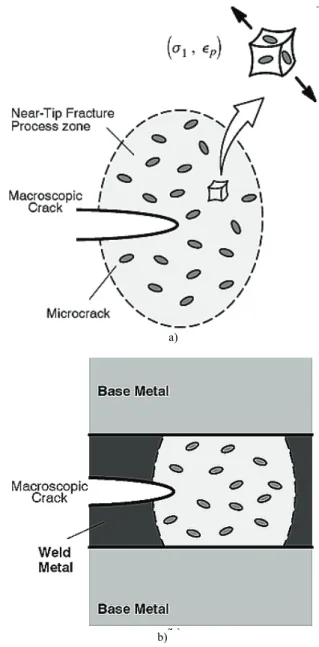
Consider an arbitrarily stressed body where a macroscopic crack lies in a homogeneous material containing randomly distributed flaws as illustrated in Fig. 1(a). The fracture process zone ahead of the crack tip is defined as the highly stressed region where the local operative mechanism for cleavage takes place; this region contains the potential sites for cleavage cracking. For the purpose of developing a probabilistic model for cleavage fracture, divide the fracture process zone ahead of crack tip in N unit volumes statistically independent, , 1, 2,..., N subjected to the principal stress . Each unit volume, , contains a substantially number of statistically independent microflaws uniformly distributed.
i V i=
1
σ Vi
The statistical nature of cleavage fracture underlies a simplified treatment for unstable crack propagation of the configuration represented in Fig. 1(a) based upon weakest link arguments. First, limit attention to the asymptotic distribution for failure of the unit volume and consider each divided into small volumes uniformly stressed, statistically independent,
i V
j V
δ , j=1, 2,..., n. Let p denote the probability of failure for the jth volume δVj. The probability that k failures occur (which correspond to the fracture of k small volume elements δV) is defined in terms of the Binomial distribution (Feller, 1957; Kendall and Stuart, 1967):
(
)
p(
1 p)
, 0 k n ,k n k S
P n ⎟⎟ k − n k ≤ ≤
⎠ ⎞ ⎜⎜ ⎝ ⎛ =
= − (3)
where denotes the total number of failures that occurred in n volume elements. When k is large and p is small, by the Poisson limit theorem (Feller, 1957; Kendall and Stuart, 1967), the distribution of the number of failures converges to a Poisson distribution with parameter
n S
μ in the form
(
)
,! k e k S P
k n
μ
μ
−
=
= (4)
where μ=kp is the expectation (mean value) of the binomial distribution. In particular, the probability that at least one failure occurs is sought. Thus, the failure probability of the unit volume, denoted P0, has distribution
(
1)
1(
0)
1 .0=PS ≥ = −PS = = −e−μ
P n n (5)
a)
b)
Figure 1. (a) Near-tip fracture process zone ahead a macroscopic crack containing randomly distributed flaws; (b) Schematic of fracture process zone for a macroscopic crack embedded in the weld metal.
To arrive at a limiting distribution for the fracture stress of a cracked solid, an appropriate functional form for the mean μ is required. The most widely adopted probabilistic model to describe fracture in brittle materials is based upon the weakest link (WL) theory. A central feature emerging from the WL model is the notion that catastrophic failure is driven by unstable propagation of a single critical microflaw or microcrack contained in the unit volume V which allows expressing the “average” number of failures, μ, as
∫
∞
=
c
l dl l g()
μ (6)
where is the microcrack size, is the critical microcrack size and g represents the microcrack density function. Here, it is understood that the failure probability p depends on the principal stress level, , acting on V, i.e., . A common assumption adopts an asymptotic distribution for the microcrack
l lc
1
density in the form g(l)=
(
ψ0 l)
ξ(Freudenthal, 1968; Evans and Langdon, 1976; Beremin, 1983), where ξ and are parameters of the distribution. However, previous fundamental work (Averbach, 1965; Tetelman and McEvily, 1967) clearly shows the strong effect of plastic deformation, in the form of inhomogeneous arrays of dislocations, on microcrack nucleation which also contributes to trigger cleavage fracture at the material's microlevel. Based upon direct observations of cleavage microcracking by plastic strain made in ferritic steels at varying temperatures (Brindley, 1970; Lindley et al., 1970; Gurland, J., 1972), the microcrack density can then be further generalized in terms of0 ψ
( )
(1 ) 0 ,ξ β γ ψ ε ⎟ ⎠ ⎞ ⎜ ⎝ ⎛ = + l l
g p (7)
where εp is the (effective) plastic strain, γ and β represent parameters defining a power law relationship between the microcrack density and plastic strain as inferred in Lindley et al. (1970).
Now, upon introducing the dependence between the critical microcrack size, lc, and (local) stress in the form lc=
(
KIc2 Y2σ12)
, where Y represents a geometry factor and is the critical stress intensity factor, and substituting Eq. (7) into Eq. (6), the mean,Ic K μ, resolves to ( ) , 0 1 1 m p ⎟⎟ ⎠ ⎞ ⎜⎜ ⎝ ⎛ Λ
=ε + σ
μ γ β (8)
where parameters m=2ξ−2 and are related to the microcrack distribution with m and . Using this result in Eq. (5) enables defining the failure probability for the unit volume V in the form
0 Λ 0 0> Λ 0 P ( ) ⎥ ⎥ ⎦ ⎤ ⎢ ⎢ ⎣ ⎡ ⎟⎟ ⎠ ⎞ ⎜⎜ ⎝ ⎛ − − = ⎥ ⎥ ⎦ ⎤ ⎢ ⎢ ⎣ ⎡ ⎟⎟ ⎠ ⎞ ⎜⎜ ⎝ ⎛ − − = + m u m u p P σ σ σ σ
εγ1 β 1 1
0
~ exp 1 exp
1 (9)
which is a Weibull distribution with parameters m and σu.
Further development in the adopted probabilistic framework requires invoking again weakest link arguments to generalize the previous probability distribution to any multiaxially stressed region, such as the fracture process zone ahead of a macroscopic crack or notch (see Fig. 1(a)). Here, the statistical problem of determining an asymptotic distribution for the fracture strength of the entire solid is equivalent to determining the distribution of the weakest unit volume V. The fundamental assumption is that the near-tip fracture process zone consists of N arbitrary and statistically independent, unit volumes V. Consequently, the failure probability of the entire cracked solid, P, is given by
[
1]
1(
1)
. 1 1 0 0∏
= − − = − − = N i N P PP (10)
Substituting Eq. (9) into the above expression and making , the probability distribution of the fracture stress for a cracked solid based upon the WL model results
∞ → N ( ) ⎥ ⎥ ⎦ ⎤ ⎢ ⎢ ⎣ ⎡ Ω ⎟⎟ ⎠ ⎞ ⎜⎜ ⎝ ⎛ Ω − − =
∫
Ω + d P m u p σ σ εγ1 β 1 01 exp
1 (11)
where denotes the volume of the near-tip fracture process zone and
Ω 0
Ω is a reference volume usually taken as unit, i.e., Ω0=1. In the present work, the active fracture process zone is defined as the loci where σ1≥λσys in which λ≈2 and σys defines the material's yield stress; results for σw differ little over a relatively wide range of λ-values for λ≈1.5~2.5. Such definition for the near-tip fracture process zone bears direct connection with the highly stressed and strained crack-tip region extending over 3~5 times the crack-tip opening displacement (δ) in which transgranular cleavage and microscopic separation processes occur (Hutchinson, 1983).
Following the development presented previously, the Weibull stress, a term coined by the Beremin group (1983) is then given by integration of the principal stress over the fracture process zone in the form
( ) m m
p w d 1 1 1 0 1 ⎥ ⎥ ⎦ ⎤ ⎢ ⎢ ⎣ ⎡ Ω Ω =
∫
Ω + σ εσ γ β (12)
from which the probability distribution given by Eq. (11) now takes the form
( )
1 exp .⎥ ⎥ ⎦ ⎤ ⎢ ⎢ ⎣ ⎡ ⎟⎟ ⎠ ⎞ ⎜⎜ ⎝ ⎛ − − = m u w w P σ σ
σ (13)
The above Eq. (13) defines a two-parameter Weibull distribution (Weibull, 1951; Mann et al., 1974) for the Weibull stress in terms of the Weibull modulus m and the scale factor . In the context of probabilistic fracture mechanics, the Weibull stress, , emerges as a near-tip fracture parameter to describe the coupling of remote loading with a micromechanics model based upon the statistics of microcracks (weakest link philosophy). A key feature of this methodology is that incorporates both the effects of stressed volume (the fracture process zone) and the potentially strong changes in the character of the near-tip stress fields due to constraint loss. The next sections address application of the Weibull stress methodology to predict effects of constraint loss and strength mismatch on cleavage fracture toughness data.
u σ w σ w σ
Toughness Scaling Methodology Based Upon the
Weibull Stress
This section introduces the essential features of a toughness scaling methodology (TSM) based upon the Weibull stress to correlate toughness values ( or CTOD) across crack configurations with varying geometries and crack-tip constraint levels, including weldments. The presentation begins with the development of a TSM strategy which appears most applicable to assess the effects of constraint and statistical variations on cleavage fracture toughness data in homogeneous materials. Subsequent description focuses on the extension of the TSM approach to bimaterial systems such as center-cracked welds.
c J
TSM for Homogeneous Materials
To make contact with the correlative character of the present framework, the concept of a toughness scaling model based upon the Weibull stress enables a simplified micromechanics treatment to predict constraint effects on cleavage fracture toughness. As discussed earlier, the central feature of this methodology derives from the interpretation of as the crack-tip driving force coupled with the simple axiom that cleavage fracture occurs when
w
σ
w
σ
reaches a critical value, σw,c. For the same material at a fixed temperature, the scaling model requires the attainment of a specified value for σw,c to trigger cleavage fracture across different crack configurations even though the loading parameter (measured by J in the present work) may vary widely due to constraint loss. In the probabilistic context adopted here, attainment of equivalent values of Weibull stress in different cracked configurations implies the same probability for cleavage fracture.
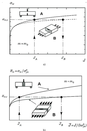
Figure 2(a) illustrates the procedure to assess the effects of constraint loss on cleavage fracture behavior needed to scale toughness values for different cracked configurations. The procedure employs J as the measure of macroscopic loading, but remains valid for other measures of remote loading, such as CTOD. Without loss of generality, Fig. 2(a) displays σw vs. J curves for a high constrained configuration (such as a deep notch three-point bend specimen – SE(B)), denoted as configuration A, and a low constraint configuration (such as surface crack specimen under tension loading – SC(T)), denoted as configuration B. Very detailed, nonlinear 3-D finite element analyses provide the functional relationship between the Weibull stress ( ) and applied loading (J) for a specified value of the Weibull modulus, . Given the -value for the high constraint fracture specimen, the lines shown on Fig. 2(a) readily illustrate the technique used to determine the corresponding -value.
w
σ
0 m m=
A J
B J
TSM for Welded Materials
TSM outlined above can be extended to assess effects of constraint variations due to weld strength mismatch on cleavage fracture toughness data by adopting the concept of a nondimensional Weibull stress, hereafter denoted σw, which is defined as σw normalized by the yield stress of the material where fracture takes place. To facilitate development of the TSM incorporating effects of weld strength mismatch, it proves convenient to first define the mismatch ratio, My, as
BM ys WM ys y M
σ σ
= (14)
where and denote the yield stress for the base metal and weld metal. Consequently, the nondimensional Weibull stress for a bimaterial system such as a welded joint can be defined as
BM ys
σ WM
ys
σ
k ys k w k w
σ σ
σ = (15)
where k=1,2 corresponds to the baseplate and weld material. In adopting such nondimensional form for the Weibull stress, it is important to emphasize that the integration appearing in Eq. (12) must be performed over the volume of the fracture process zone for each material, as depicted in Figure 1(b). With the Weibull stress defined in this manner, material points outside the region over which the integration is carried out are (implicitly) assigned a zero probability of cleavage fracture.
a)
b)
Figure 2. (a) Scaling procedure based on the Weibull stress to correct toughness values for different crack configurations. (b) Scaling procedure based on the normalized Weibull stress to correct toughness values for different mismatch conditions.
values for cracked configurations with different mismatch conditions based upon the TSM strategy. The procedure employs a nondimensional crack driving force defined by J=J
( )
bσkys , where b is the remaining crack ligament as the measure of macroscopic loading, but remains valid for other measures of remote loading, such as CTOD. Without loss of generality, Fig. 2(b) displays σw vs. J curves for a high constraint, welded configuration (such as a deep notch SE(B) specimen with a center-cracked square groove) made with an evenmatch condition ( 1 ), denoted as configuration A, and a welded structural component (such as surface crack specimen under tension loading) made with an overmatch condition ( ), denoted as configuration B. Again, very detailed, nonlinear 3-D finite element analyses provide the functional relationship between the Weibull stress (=
y M
1
>
y M
w
σ ) and applied loading (J ) for a specified value of the Weibull modulus, . Given a measured toughness value at cleavage for the high constraint, evenmatch fracture specimen (
0 m m=
A
J ), the lines shown on Fig. 2(b) readily illustrate the technique used to determine the corresponding JB-value for the structural welded component.
A key assumption in the above toughness scaling methodology is that parameter is independent of strength mismatch level, , or, at least, it can be considered a weak function of the mismatch ratio. For low to moderate levels of weld overmatch ( 3 ), the adopted assumption appears consistent with the development pursued in this work while, at the same time, maintaining the relative simplicity of TSM to welded components given current knowledge. As will be discussed, the adopted engineering procedure is rather effective in predicting the failure strain of a 10% overmatch wide plate specimen even though its level of crack-tip constraint varies widely from a conventional, laboratory fracture specimen under bending.
m
y M
. 1 ~ 2 . 1
≤
y M
Parameter Calibration of the Weibull Modulus, m, Using
Toughness Data
Calibration of the material dependent m-parameter, and to a lesser extent parameters γ and β describing the potential influence of plastic strain on microcrack density, plays a crucial role in applications of the present methodology to assess effects of constraint and statistical variations on cleavage fracture toughness data. In particular, the Weibull modulus, m, strongly affects the shape and magnitude of the constraint correction curves upon which the toughness ratio for two different crack configurations is determined (see Fig. 2).
The calibration protocol scheme for parameter m adopts the scaling methodology previously outlined to correct measured toughness distributions for different crack configurations. The procedure extends previous work by Gao et al. (1998) and Ruggieri et al. (2000) to calibrate the Weibull modulus using high constraint (SSY) and low constraint (LSY) fracture toughness data measured at the same temperature and loading rate. Because each measured -value is corrected to its equivalent -value, the statistical (Weibull) distribution of -values is also corrected to an equivalent statistical (Weibull) distribution of -values. Consequently, the present scheme defines the calibrated m-value for the material as the value that corrects the characteristic toughness
(i.e., the scale parameter of previous Eq. (2)) to its equivalent for two sets of fracture toughness data from different crack configurations and with sufficient differences in the evolution of
A c
J JcB
A c J
B c J
A J0
B J0
w
σ vs. J. The procedure can also be extended in straightforward manner to calibrate parameter m for weldments and bimaterial systems.
The following steps describe the key procedures in the adopted calibration scheme for parameter m. The next section addresses application of this parameter calibration process for ferritic structural steels, including overmatched welds.
Step 1
Test two sets of specimens with different crack configurations (A and B) in the ductile-to-brittle transition (DBT) region to generate two distributions of fracture toughness data. Select the specimen geometries and the common test temperature to insure different evolutions of constraint levels for the two configurations. No ductile tearing should develop prior to cleavage fracture in either set of tests. For weldments, test two sets of specimens with different strength mismatch conditions (A and B) also in the region to generate two distributions of fracture toughness data. Ideally, configuration A should correspond to fracture specimens for the evenmatch condition (My=1). Several alternatives to obtain the two sets of toughness values at the same test temperature include: i) for homogeneous materials, test high constraint deep-notch SE(B)s or C(T)s specimens with aW≥0.5 as configuration A. To ensure SSY conditions at fracture, set the specimen size so that
M b
Jc≤ σys for each specimen, with the deformation limit, M, conservatively set to
≈
60~100 (Nevalainen and Dodds, 1995). For configuration B, use similar size SE(B) specimens, but with shallow-notches, i.e., aW≤0.2~0.25. These will undergo significant constraint loss when the deep-notch values just satisfy the suggested deformation limit; ii) for weldments, test deep-notch SE(B)s or C(T)s specimens with aW≥0.5and different degrees of weld mismatch. Select the specimen geometries, mismatch conditions and the common test temperature to insure different evolutions of mismatch and constraint levels for the two configurations.Step 2
Determine the characteristic toughness value for each data set, and , using a standard maximum likelihood estimation procedure (Mann et al., 1974). Alternatively, the Master Curve procedure given by ASTM E-1921 (ASTM, 2008) can be employed with the fracture toughness measure, , replaced by which enables defining in the form
A
J0 J0B
Jc
K Jc
0 J
2 1
1 2
, 0
1
⎥ ⎥ ⎦ ⎤ ⎢
⎢ ⎣ ⎡
=
∑
= J
N
i i c J
J N
J (16)
where is the number of tested specimens for each crack configuration. In the above formulation, it is understood that the threshold fracture toughness, , is set equal to zero and the Weibull modulus,
J N
th J
be treated as censored values by manipulating the Master Curve procedure as above (see ASTM E-1921) in the form
2 1
1 2
, 0
1
⎥ ⎥ ⎦ ⎤ ⎢
⎢ ⎣ ⎡
=
∑
= J
N
i i c J r
J (17)
where r is now the number of tested specimens exhibiting no ductile tearing.
Step 3
Perform detailed, nonlinear finite element analyses in large geometry change (LGC) setting for the tested specimen geometries. The mesh refinements must be sufficient to ensure converged vs. (or
w
σ
J σw vs. J ) histories for the expected range of m-values and loading levels.
Step 4
4.1 Assume an m-value. Compute the σw vs. J (or σw vs. J ) trajectories for configurations A and B to construct the toughness scaling model relative to both configurations.
4.2 Correct J0A (J0A) to its equivalent J0B (J0B), i.e., the corrected value of the mean toughness for the assumed m-value for effects of constraint loss or weld strength mismatch. Define the error of toughness scaling as
(
A A)
Am J J
J m
R( )= 0, − 0 0 or
(
A A)
A m J J Jm
R( )= 0, − 0 0 .
4.3 If , repeat substeps 4.1-4.2 for additional m -values. The calibrated Weibull modulus, , makes
0 ) (m ≠ R
0 m
m= R(m)=0 within a small tolerance.
Numerical Procedures and Computational Models
Finite Element Models for Homogeneous Fracture Specimens
Three-dimensional finite element analyses are conducted on different crack configurations which include: (1) a conventional, plane sided C(T) specimen with aW=0.6, 25B= mm and
mm; (2) a conventional, plane sided SE(B) specimen with 50
=
W 2 . 0
=
W
a , mm, mm and and (3) a bolt-loaded surface crack SC(T) specimen with
25
=
B W=50 S=4W
25 . 0
=
t
a , c a=3and mm. For the C(T) and SE(B) specimens, a is the crack length, W is the specimen width, B is the specimen thickness and S is the bend specimen span. For the SC(T) specimen, a is the maximum depth of the surface crack, 2c is the length of the semi-elliptical crack and t is the thickness of the cracked section. Figure 3 shows the geometry and specimen dimensions for the analyzed crack configurations. Joyce and Link (1997) used these specimens to measure the cleavage fracture resistance of an ASTM A515-70 pressure vessel steel.
25
=
t
Figure 3. Geometry of tested specimens for A515-70 pressure vessel steel.
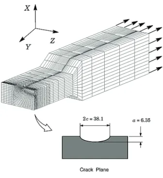
Figure 4 displays the finite element model constructed for the 3-D analyses of the SC(T) specimen. Symmetry conditions enable analyses using one-quarter of the 3-D model with appropriate constraints imposed on the symmetry planes. A focused ring of elements surrounding the crack front in the radial direction is used with a small key-hole at the crack tip; the radius of the key-hole,
0
ρ , is 2.5μmm. The half-length of the semi-elliptical crack is defined by 20 elements arranged over the (one-half) crack front. The quarter-symmetric, 3-D model for the SC(T) specimens has 25650 nodes and 22800 elements. The models for the C(T) and SE(B) specimens have similar features and similar levels of mesh refinement. These meshes have 10 variable thickness layers defined over the half-thickness (B 2); the thickest layer is defined at Z=0with thinner layers defined near the free surface (Z =B 2) to accommodate strong Z variations in the stress distribution. The quarter-symmetric, 3-D models for the C(T) and SE(B) specimens have 11800 nodes and 9800 elements.
Finite Element Models for Welded Fracture Specimens
Three-dimensional nonlinear finite element analyses are also conducted on different welded crack configurations which include: (1) a conventional, plane sided SE(B) specimen with aW =0.5,
25
=
B mm, 25W= mm and and (2) a clamped surface crack SC(T) specimen with
W S=4
=
t
a 0.24, at=8.3, 25t= mm, 400
Figure 4. Quarter-symmetric finite element model for the bolt-loaded surface crack specimen.
Figure 6 displays the finite element model constructed for the 3-D analyses of the SC(T) specimen. Symmetry conditions enable analyses using one-quarter of the numerical model with appropriate constraints imposed on the symmetry planes. Again, a focused ring of elements surrounding the crack front in the radial direction is used with a small key-hole at the crack tip; the radius of the key-hole, , is also 50 mm with similar levels of refinement along the crack front that closely match the mesh refinement employed in the SE(B) specimen. The half-length of the semi-elliptical crack is defined by 16 elements arranged over the (one-half) crack front. The quarter-symmetric, 3-D model for the SC(T) specimens has ~6300 8-node, 3D elements (~7500 nodes). This finite element model is loaded by displacement increments imposed on the loading points with clamped constraint conditions at the specimen ends. The models for the SE(B) specimens have similar features and similar levels of mesh refinement. The quarter-symmetric, 3-D meshes have 12 variable thickness layers with ~10000 8-node, 3D elements (~12000 nodes) defined over the half-thickness (
0 ρ
2
B ); the thickest layer is defined at with thinner layers defined near the free surface (
0
=
Z 2 B
Z= ) to accommodate strong Z variations in the stress distribution.
Material Models and Computational Procedures
The elastic-plastic constitutive models employed in all analyses reported here follow a flow theory with conventional Mises plasticity in large geometry change (LGC) setting. The next section describes numerical analyses for fracture specimens extracted from an A515-70 pressure vessel and an API X80 pipeline steel weld that were tested in the experimental program. Gao et al. (1999) describes the uniaxial stress-strain curve for the A515-70 pressure vessel steel at the test temperature,
2 J
7
− =
T °C and °C. Minami et al. (1995) provides the uniaxial true
stress vs. logarithm strain curves for the API X80 pipeline steel (base plate and overmatch weld material) at the test temperature,
28
− =
T
5
− =
T °C. These curves for both materials were used in the finite element computations reported here.
Figure 5. Geometries for the tested welded fracture specimens.
Figure 6. Finite element model for the SC(T) specimen.
The numerical computations for the cracked configurations reported here are generated using the research code WARP3D (Gullerud et al., 2004). The code incorporates a Mises ( ) constitutive model in both small-strain and finite-strain framework and solves the equilibrium equations at each iteration using a very efficient, sparse matrix solver highly tuned for Unix and PC based architectures. This sparse solver significantly reduces both memory and CPU time required for solution of the linearized equations
compared to conventional direct solvers. A typical 3-D analysis for solution of the fracture models employed in this study runs in two to six hours in a single-processor PC-based workstation. The finite element computations employ a domain integral procedure (Moran and Shih, 1987) for numerical evaluation of the J integral along the crack front. The research code WSTRESS (Ruggieri, 2001) is used to construct σw vs. J (σw vs. J ) trajectories for these fracture specimens needed to perform the calibration of parameter m.
Cleavage Fracture Predictions for the A515-70 Pressure
Vessel Steel
Fracture Toughness Testing
Joyce and Link (1997) and Gao et al. (1999) recently reported a series of fracture toughness tests conducted on an ASTM A515 Gr70 pressure vessel steel. The fracture mechanics tests include: (1) a conventional, plane sided C(T) specimen with aW=0.6, mm and mm; (2) a conventional, plane sided SE(B) specimen with
25
=
B W=50
2 . 0
=
W
a , mm, mm and
and (3) a bolt-loaded surface crack SC(T) specimen with 25
=
B W =50
W S=4
25 . 0
=
t
a , c a=3and mm. The material is an A515-70 pressure vessel steel (280 MPa yield stress at °C) with relatively high hardening properties (
25
=
t
7
−
2
≈
ys uts σ
σ ). Gao et al. (1999) provides the true stress-logarithmic strain curve at the test temperatures ( °C and °C) for this material used in the finite element analyses of the specimens.
7
− =
T T=−28
Testing of these configurations was performed at T=−28°C for the C(T) specimens and °C for the SE(B) and SC(T) specimens; these temperatures correspond to the ductile-to-brittle transition behavior for the material. Figure 7(a) provides a Weibull diagram of the measured toughness values for both test temperatures. The solid symbols in the plots indicate the experimental fracture toughness data for the specimens. Values of cumulative probability, F, are obtained by ordering the -values and using
7
− =
T
c J
(
−0.3) (
+0.4)
= i NJ
F , where i denotes the rank number and defines the total number of experimental toughness values. The straight lines indicate the two-parameter Weibull distribution, Eq. (1). While the Weibull slopes for the C(T) and SE(B) toughness distributions are very similar (
J N
2
≈
α for both distributions), the results clearly demonstrate a strong effect of constraint level on the characteristic toughness, (the -value corresponding to 63.2% failure probability). In contrast, the Weibull slope for the SC(T) specimen differ significantly (
0
J J
10
≈
α ) from the α-value for the C(T) and SE(B) specimens; here, the SC(T) and shallow crack SE(B) specimen have similar values for the characteristic toughness.
a)
b)
Figure 7. (a) Weibull plots of experimental toughness values at temperatures −7°C and −28°C for the A515-70 pressure vessel steel; (b) Cleavage fracture predictions for the SC(T) specimen at −7°C for the A515-70 pressure vessel steel.
Parameter Calibration
The parameter calibration scheme described earlier is applied to determine the Weibull stress parameters for the tested pressure vessel steel. Here, the plastic strain correction is not adopted, so that
=
γ 0 in previous Eq. (12) defining the Weibull stress. The Weibull modulus, , is calibrated using the deep notch C(T) specimens and the shallow notch SE(B) specimens. Because the specimens were not tested at the same temperature, the present methodology adopts a simple procedure to correct the measured toughness values for temperature. By using the Master Curve procedure given by ASTM E-1921 (ASTM, 2008), the -value for the C(T) specimens at
m
0 J
28
− =
T °C is scaled to corresponding J0-value at T=−7°C. Moreover, since the toughness values for this specimen are below the limit value KJc= Eb0σ0 M with the deformation limit
30
=
M given by ASTM E-1921, they are taken directly as SSY toughness values at T=−28°C. The characteristic toughness values for the C(T) and SE(B) specimens at °C are then given as:
54 kJ/m
7
− =
T
≈ ) ( 0
T C
a)
b)
Figure 8. Calibration procedure for the Weibull modulus, m, using constraint correction curves at −7°C for the A515-70 pressure vessel steel: (a) C(T) specimen; (b) SE(B) specimen.
With the toughness values for the C(T) and SE(B) specimens set at the same temperature (T=−7°C) and using σw vs. curves constructed from the 3-D finite element analyses for both crack configurations, the calibration procedure is then applied to determine the -value that yields the same
J
m σw-value for the pair ( , ). Figure 8 provides constraint correction curves, vs. and vs. , for both specimen geometries with different m-values. The calibration process is illustrated in the plot by solid lines which indicate the -value that produces a unique value corresponding to the pair ( , ) at °C. Here, the calibrated Weibull modulus for the tested A515 pressure vessel steel is
) ( 0CT
J J0SE(B)
SSY
J JC(T) JSSY JSE(B)
m SSY
J0
) ( 0
T C
J J0SE(B) T=−7
≈
m 8.
Fracture Predictions
To verify the predictive capability of the Weibull stress methodology adopted in the present work, this section describes application of the toughness scaling model based on the Weibull stress (σw) to predict the toughness distribution for the bolt-loaded surface crack specimen. Very detailed 3-D, nonlinear finite element analyses provide crack front stress fields to generate the evolution
of σw vs. for the -value calibrated in the previous section. Here, because the crack front length of the SC(T) specimen equals 1.67 times the crack front length of the 1(T) specimens (Weisstein, 2010), the corresponding Weibull stress must be scaled to the length of the semi-elliptical crack front.
J m
The Weibull probability plot in Fig. 7(b) shows the predicted distributions of cleavage fracture toughness for the bolt-loaded surface crack specimen. The solid symbols in the plot indicate the measured cleavage fracture toughness ( ) for this specimen. Values of cumulative probability, F, are obtained by ordering the
-values and using
c J
c
J F=
(
i−0.3) (
NJ+0.4)
, where denotes the rank number and defines the total number of experimental toughness values. The solid line on each figure represents the predicted Weibull distribution generated from the distribution (not individual values from tested specimens) of toughness values for the C(T) specimen withi
J N
=
W
a 0.6 using a Monte Carlo procedure (Mann et al., 1974). The dashed lines represent the 90% confidence bounds generated from the 90% confidence limits for the calibrated
-value (Thoman et al., 1969). m
The effectiveness of the present model in describing general fracture behavior for this specimen is clear as the predicted distribution of fracture toughness displayed in Fig. 7(b) agrees well with the experimental data. Here, the 90% confidence bounds bracket most of the measured toughness values in the mid-region of the curves. The results also indicate that the predicted curves: (1) overpredict the failure probability in the lower tail of the plots and (2) underpredict the failure probability in the upper tail of the plots. However, it should be emphasized that the toughness distribution for the bolt-loaded SC(T) specimen differs significantly from the toughness distribution for the shallow notch SE(B) specimen even though both specimens have similar levels of characteristic toughness (recall that the Weibull slopes for the toughness distributions of these specimens displayed in Fig. 7(a) are very different). Nevertheless, the overall error appears sufficiently small to support application of the Weibull stress methodology in the fracture predictions analyzed here.
Prediction of Failure Load in the API X80 Girth Weld
Experimental Program
Minami et al. (1995) reported on a series of fracture tests conducted on weld specimens made of an API X80 pipeline steel. The welding procedure and welding conditions follow closely those employed in girth welds made in field conditions. Figure 5 shows the tested weld configurations which include deeply notched SE(B) fracture specimens and a wide plate SC(T) specimen with a semi-elliptical, surface center crack with varying levels of weld strength mismatch: evenmatch ( 1.02) and 10% overmatch (
=
y M
=
y
M 1.09). The SE(B) specimens have aW=0.5 with thickness
=
B 25 mm, width W=25 mm and span distance S=100 mm. The wide plate specimens have thickness t=25 mm, width 2W=400 mm and length L=300 mm; here, the surface crack has length
=
c
2 100 mm and depth a=6 mm (at=0.24 and c a=8.3). In all fracture specimens, the weld groove width, 2h, is 10 mm.
The weld specimens were prepared using standard GMAW procedure with heat inputs ranging from 0.3 to 0.9 kJ/mm according to the pass sequence (see details in Minami et al., 1995). Mechanical tensile tests extracted from the longitudinal weld direction provide the stress-strain data at room ( °C) and test temperature (
20 5
yield stress, σys=581 Mpa, and tensile strength, σuts=670 MPa. The 10% overmatch weld has yield stress, σys=621 MPa, and tensile strength, σuts=691 MPa. The degree of weld strength mismatch is essentially similar to the mismatch level at room temperature. Moreover, both materials display relatively low strain hardening (σuts σys≈1.11~1.15) so that effects of hardening mismatch are considered negligible. Other mechanical properties for this material include Young's modulus, E=206 GPa and Poisson's ratio, ν=0.3. Minami et al. (1995) provide further details on the mechanical tensile test data for this material.
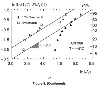
Testing of the SE(B) specimens was performed at T=−5°C which is within the range of the ductile-to-brittle transition behavior for the material. Records of load vs. crack mouth opening displacements (CMOD) were obtained for each specimen using a clip gauge mounted on knife edges attached to the specimen surface. Post-test examinations established the amount of stable crack growth prior to final fracture by cleavage. Figure 9(a) shows the effect of strength mismatch on the measured -values. The toughness values for the 10% overmatch specimens exceed the evenmatch toughness by a factor of 1.5~2.0. Figure 9(b) provides a Weibull diagram of the measured toughness values for both sets of data. The solid symbols in the plot indicate the measured cleavage fracture toughness ( ) for this specimen. Values of cumulative probability, F, are obtained by ordering the -values and using
c J
c J
c J
(
−0.3) (
+0.4)
= i NJ
F , where i denotes the rank number and defines the total number of experimental toughness values. The straight lines indicate the two-parameter Weibull distribution, Eq. (1) with 0, obtained by a maximum likelihood analysis (Mann et al., 1974) of the data set with a fixed Weibull slope of
J N
=
th J
= α 2. Fracture testing was also conducted on the wide plate specimens with a 10% overmatch girth weld at °C. Records of overall (remote) strain, , vs. crack mouth opening displacements (CMOD) were obtained using 4 strain gages conveniently attached at a distance of 100 mm from the notch on both sides of the plate. The specimen failed by overload fracture after some amount of ductile tearing; here, the experimentally measured failure strain (average of the strain gage readings) is given by
5
− =
T
r
ε
=
f
ε 2.25% (Minami et al., 1995).
a)
Figure 9. (a) Experimental toughness values for welded deep crack SE(B) fracture specimens of API X80 steel with two mismatch (5°C); (b) Weibull distribution of toughness values for the experimental data set of the SE(B) fracture specimens.
b)
Figure 9. (Continued).
Weibull Modulus Calibration for the Tested Weldment
The parameter calibration scheme described previously is applied to determine the Weibull modulus for the tested weldment. In the present application, calibration of parameter is conducted by scaling the mean value of the measured toughness distribution for the evenmatch SE(B) specimen (taken here as the "baseline" value) to an equivalent mean value of the toughness distribution for the 10% overmatch SE(B) specimen. The calibration process simply becomes a means of determining an -value that corrects the nondimensional characteristic toughness value for the evenmatch specimen, denoted
m
m
Even B SE
J0, ( ), to its equivalent value for overmatch specimen, JOver0,SE(B).
As further refinement, the procedure also considers the influence of the plastic strain correction on the Weibull stress and, consequently, on the calibrated Weibull modulus for the tested material. For the purpose of assessing the effectiveness of Eq. (12) in predictions of the failure strain for the wide plated conducted next, the present investigation considers two sets of widely different parameters defining the microcrack density: i) γ=0 (no plastic strain correction) and ii) γ=1 and β=0 which implies a simple linear dependence of microcrack density on the plastic strain. While this choice of parameters γ and β is somewhat arbitrary, it does make contact with the experimental findings of Lindley et al. (1970) and Gurland (1972) in ferritic steels.
Very detailed finite element computations of these specimens enable construction of the J0Even,SE(B)→J0Over,SE(B) correction shown in Fig. 10(a)-(b) for varying -values. In both plots, each curve provides pairs of -values corresponding to the 10% overmatch and evenmatch SE(B) specimen that produce the same nondimensional
m J
w
σ . The Weibull modulus does affect predictions of mismatch effects; here, changing the -value assigns a different weight factor to stresses at locations very near to the crack front thereby altering the ratio of mismatch correction. A closer inspection of these plots also reveals that the toughness scaling curves for the fracture specimens and mismatch levels considered display only a weak dependence on the adopted plastic strain correction. Because the crack geometry and degree of mismatch for both fracture specimens do not differ significantly, this behavior is not unexpected since the near-tip strain fields for both the evenmatch and overmatch specimens under analysis should be relatively similar.
The calibration scheme now proceeds by adopting a two-parameter Weibull function given by Eq. (1) with α=2 and 0 to describe the toughness distribution. Here, the characteristic toughness values for the evenmatch and overmatch bend specimens are 67 kJ/m
=
th J
≈
Even B SE
J0, ( ) 2 and J0Over,SE(B)≈ 118 kJ/m2. Once the -values for each mismatch condition is determined, the calibration procedure then yields the Weibull modulus of the tested material at
°C for the two cases considered in the present study: i) 13.5 for
m
5
− =
T
=
m γ=0 (no plastic strain correction) and ii) m=15.0 for
=
γ 1 and β=0 (linear plastic strain correction). Figure 10 recasts the calibration strategy into a graphical procedure for both cases considered to determine parameter using the scaling curves displayed in that plot. Again, these calibrated -values are similar and exhibit a relatively minor dependence on the adopted plastic strain correction.
m m
Failure Strain Prediction for the Welded Plate
To verify the predictive capability of the Weibull stress methodology adopted in the present work, this section describes application of the toughness scaling model based on the nondimensional Weibull stress (σw) incorporating effects of weld strength mismatch and plastic strain to predict the failure strain for the clamped surface crack SC(T) specimen with 10% overmatch. Very detailed nonlinear finite element analyses provide the crack front stress fields to generate the evolution of σwvs. J for the -values calibrated in the previous section. Here, the -value at failure for the tested SC(T) specimen,
m J
Over T SC
J0, ( ), and the
corresponding failure strain are predicted using the measured deep crack toughness values for the evenmatched SE(B) specimen translated in terms of the (nondimensional) characteristic toughness,
Even B SE J0, ( ).
Figures 11(a)-(b) show the computed evolution of σw under increasing values of J for the SE(B) and SC(T) configurations using the plastic strain correction model with the calibrated -values. Figure 12 displays the mechanical response of the SC(T) specimen characterized in terms of the evolution of remote applied strain, , with increased (nondimensional) crack-tip loading,
m
r
ε J .
These curves provide the quantitative basis to predict the failure strain for the surface crack specimen with 10% overmatch. Here, because the crack front length of the SC(T) specimen is 4 times the crack front length of the SE(B) specimen (Weisstein, 2010), the
w
σ -values for the bend specimen must be scaled to the length of the semi-elliptical crack front for the wide plate specimen to guarantee that similar volumes of the (near-tip) fracture process zone are included into the computation of the Weibull stress for each crack configuration (see Eq. (12)).
a)
b)
Figure 10. Toughness correction using the TSM methodology based upon the nondimensional Weibull stress with varying Weibull moduli for the tested welded SE(B) fracture specimens.
a)
b)
Figure 11. (Continued).
Figure 12. Evolution of remote applied strain with increased nondimensional J for overmatch SC(T) specimen.
Using again the TSM procedure outlined previously, prediction of the failure strain for the SC(T) specimen proceeds as follows. First, the characteristic J0-value for the 10% overmatch SC(T) specimen is determined based upon the J0-value for the evenmatch SE(B) specimen. The failure strain is then evaluated by means of the computed strain-crack driving force relationship for the wide plate specimen. As a further refinement, the 90% confidence limits for the J0-value of the evenmatch SE(B) specimen are also employed to estimate the corresponding 90% confidence bounds for the failure strain of the SC(T) specimen.
Consider first the nondimensional Weibull stress trajectories with no plastic strain correction displayed in Fig. 11(a). While σw for the evenmatch SE(B) specimen shows a marked increase with
J , the Weibull stress for the SC(T) specimen rises at a much lower rate with increased levels of crack-tip loading. Given the expected toughness ratio ( OverSCT
Even B SE J
J0, ( ) 0, ( )) of ≈10~15 for these two data
sets, the analysis clearly fails to predict the failure strain for the SC(T) specimen. Consider now the evolution of σw vs. J incorporating the effect of plastic strain displayed in Fig. 11(b). With the introduction of the adopted plastic strain correction, a different picture now emerges which can be summarized as follows:
1) The σw vs. J trajectory for the evenmatch SE(B) specimen increases rapidly in the initial stage of crack-tip deformation and then more slowly as crack-tip deformation continues and 2) The overmatch SC(T) specimen also displays a slowly rising Weibull stress curve, but which is now fully consistent with the toughness ratio for the analyzed data sets. Based upon the σw vs.
J trajectories displayed in Fig. 11(b) and the plot of εrvs. J displayed in Fig. 12, the predicted failure strain, εpred, and corresponding 90% confidence bounds (Thoman et al., 1969) are
=
pred
ε 2.27% (1.2%; 3,6%). Even though Minami et al. (1995) report only a single value for the experimental failure strain, the ability of the present model in describing the fracture behavior for the overmatch SC(T) specimen seems evident as the predicted failure strain and the 90% confidence bounds agree very well with the experimental data.
Summary and Conclusions
This work describes the development of a probabilistic framework and a toughness scaling methodology incorporating the effects of constraint loss and weld strength mismatch on crack-tip driving forces. The approach builds upon a micromechanics description of the cleavage fracture process using the Weibull stress,
, as a near-tip driving force coupled to a convenient description of the toughness scaling model. For the same material at a fixed temperature, the scaling model requires the attainment of a specified value for to trigger cleavage fracture across cracked configurations, including weldments, even though the corresponding J (
w
σ
w
σ
δ)-values may differ widely. A key feature of this methodology is that incorporates both the effects of stressed volume (the fracture process zone) and the potentially strong changes in the character of the near-tip stress fields due to constraint loss (and weld strength mismatch). The procedure is naturally suited for implementations coupled with finite element codes so that different constitutive properties as well as strain rate and thermal effects can easily be addressed. Application of the methodology to predict cleavage fracture behavior in pressure vessel steel tested in the transition region agrees well with experimental data. Moreover, extension of the procedure to predict the failure strain for an overmatch girth weld made of an API X80 pipeline steel clearly demonstrates the effectiveness of the micromechanics approach. Overall, the results lend strong support to use a Weibull stress based procedure in defect assessments of structural components.
w
σ
Acknowledgements
This investigation is supported by the Brazilian Council for Scientific and Technological Development (CNPq). The author acknowledges Prof. F. Minami from Osaka University for making the girth weld data for the API X80 steel available.
References
Al-Ani, A.M., and Hancock, J.W., 1991, “J-Dominance of Short Cracks in Tension and Bending”, Journal of Mechanics and Physics of Solids, Vol. 39, pp. 23-43.
American Society for Testing and Materials, 2008, “Standard Test Methods for Determination of Reference Temperature, T0, for Ferritic Steels in the Transition Range”, ASTM E-1921, Philadelphia.
Anderson, T.L., 2005, “Fracture Mechanics: Fundaments and Applications” - 3rd Edition, CRC Press, New York.
Averbach, B.L., 1965, “Micro and Macro Crack Formation”,