Abstract—State estimation is widely used in the field of process system engineering. There are several available technologies regarding this topic, e.g. Extended Kalman Filter (EKF). The EKF is the variant of the standard Kalman filter and is successfully applied on the nonlinear systems for state estimation. As well known, the PEMFC is a typical nonlinear system, and some of the internal states are obtained costly, and even cannot be measured directly. Hence, in order to obtain these internal states effectively via collecting measurable variables, the EKF is applied in this study. The goal of this paper is to demonstrate the implementation of the EKF based on a PEMFC model which is taken in a literature, in order to estimate the following internal states: concentrations of vapor and oxygen in cathode chamber, as well as cell temperature. The corresponding results show that the EKF can serve as a ‘software sensor’ for the control design or the supervision in the fuel cell system.
Index Terms—State estimation, Extended Kalman filter, PEMFC system
I. INTRODUCTION
S well known, not all the states in a chemical process are easily obtained. The state estimation could be a costless solution to access these states via state estimation techniques. For the linear system, the state estimation can be done by the Kalman Filter (KF) because the probability distribution function (pdf) of the system state is propagated in an optimal way. However, the KF is not suitable for the nonlinear systems. An alternative solution is a variant of the standard KF, e.g. extended Kalman filter (EKF) or unscented Kalman filter (UKF). It is known that there exists no perfect solution that is superior to other techniques of state estimation. The main principle of choosing an estimation method is to trade off various aspects such as accuracy of estimation, difficulty of implementation, numerical robustness, and computational load[1].
Manuscript received Nov.23, 2011. This work was supported by Higher innovative talent recruitment program (B08019) and Shanghai Leading Academic Discipline Project (B303).
Jichen Liu is with School of Automotive Studies, Tongji University, Shanghai, 201804 China (e-mail: [email protected]).
Guangji Ji is with School of Automotive Studies, Tongji University, Shanghai, 201804 China (e-mail:[email protected]), corresponding author.
Su Zhou is with School of Automotive Studies/ Clean Energy Automotive Engineering Center/ Sino-German Postgraduate School, Tongji University, Shanghai, 201804 China (e-mail: [email protected]).
The EKF with different applications encounter in several literatures. Dan Simon [2] briefly introduced the mentioned different kinds of state estimation methods and their basic principles, respectively. By comparing these methods, the EKF is one of the most widely used and attractive methods owing to its relative simplicity and efficacy for nonlinear system. Kandepu et al. [3] depicted the principle of the EKF, and four nonlinear cases were introduced: the first one is the Van der Pol oscillator. The second is an estimation problem in an induction machine. The third is the state estimation in a reversible reaction. Finally, a hybrid solid oxide fuel cell (SOFC) system is introduced to evaluate the performance of the EKF. In the literature [4], an evaluation of the EKF was given by comparing to the moving horizon estimation (MHE). It turned out that, the computational load required to solve the MHE is greater than the EKF. For the differential algebraic equation (DAE) system, the EKF can be used through the proper modifications as well [5].
The combination of the EKF and the fuel cell system can be also found in several literatures. It is known that the fuel cell system is a strong nonlinear system. Some internal states in the system (e.g. cathode side relative humidity (RH)) would be detected costly by the delicate sensors. To reduce the cost of the system, those sensors can be removed by using the EKF. Some internal states (e.g. oxygen partial pressure and cell temperature) cannot be directly measured by sensors and could be estimated via the EKF as well. Recently, some studies concerning on the state estimation in the fuel cell systems have been carried out. Groetsch et al. [6] applied the EKF which is designed on the basis of the reduced model of a molten carbonate fuel cell (MCFC) system. The EKF was tested by both simulations and experiments. It is stated the temperature sensors in the stack as well as the expensive concentration measuring equipments can be removed. Kandepu et al. [7] used both UKF and EKF methods on the SOFC system to estimate the stack temperature. Suares et al. [8] used a nonlinear programming (NLP) formulation for both the parameter and state estimation in a PEMFC. Goerguen et al. [9] proposed a novel method for estimation of the inside humidity by exploiting its effect on cell resistive voltage drop. There are seldom studies reporting the applications of EKF in the PEMFC system. Hence, the main motivation of this paper is to apply the EKF and describe its implementation in PEM fuel cell system with considerable clear manner.
The organization of this paper is as follows. In section 2 the fundamental theory of Kalman filter and EKF is
Applying and Implementation of the Extended
Kalman Filter (EKF) with Sensitive Equation:
A PEMFC Case Study
Jichen Liu, Guangji Ji*, Su Zhou
illustrated by using an example of a nonlinear system. In Section 3 the EKF is tested via a PEMFC system. The introduction of the fuel cell system model, implementation of the EKF technique and the simulation results are included. Finally, the conclusions are drawn in Section 4.
II. FUNDAMENTAL THEORY OF THE KF AND THE EKF A. Principle of the KF
The KF is the minimum-variance state estimator, no matter with- or without Gaussian noise [3]. To illustrate the principle of the KF, the following linear discrete-time system is taken into account. The model equations are given in (1) and (2):
1
k k k
x Fx w 1
k k k
y Hx v 2
where
k
is the time step,x
k represents the state to be estimated at timek
,y
k is the measurement at timek
,w
k andv
k are the zero-mean process noise and measurement noise with co-variances Q and R, respectively, i.e.[ k Tk]
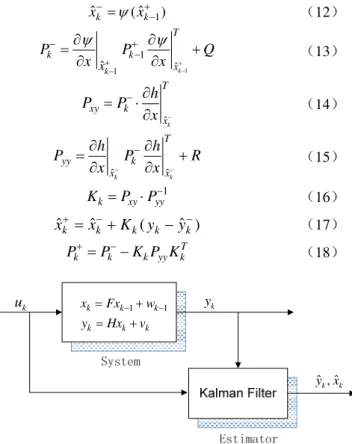
E w w Q,E v v[ k kT]R,E w[ k]E v[ k]0, F and H are the state transition and measurement matrix, which represent the essential characteristics of the system. Fig.1 shows the framework of state estimation. It is assumed that the system can be observable fully, and the KF formulations for the states are given as follows [3]:
1
T
k k
PFPF Q 3
1
ˆk ˆk
x Fx 4
( )
k k k
P IK H P 5
ˆk ˆk k( k ˆk)
x xK y Hx 6
1
( )
T T
k k k
K P H HP H R 7
where k1, 2,...
I
is the identity matrix,x
ˆ
k is the priori estimation of the statex
k,x
ˆ
k is the posteriori estimation of the state, Kkis the Kalman gain, Pkis the covariance of the priori estimation errorx
k
x
ˆ
k. Pkis the covariance of the posteriori estimation errorx
k
x
ˆ
k. The initialization of the KF is written as:0 0
ˆ ( )
xE x 8
0 [( 0 ˆ0)( 0 ˆ0) ]
T
PE x x x x 9
Generally there are two main steps in KF. The first step is called ‘prediction step’, as shown in (3) and (4). The second step is called ‘update step’, shown in (5), (6) and (7).
B. Introduction of the EKF via an exemplary nonlinear model
The KF is the unbiased estimation for the linear model [3]. For the nonlinear model, the expectation of the nonlinear function cannot be easily obtained. Under this situation, the EKF can be derived when the nonlinear model is linearized and the expectation can be approximated as the linear function of the estimated state. The main disadvantage of linearization lies in biased estimation and insufficient
accuracy. However, for the state estimation in nonlinear systems, the EKF has several attractive features because it can be easily understood and implemented. In this study, the EKF is firstly illustrated with a discrete-time nonlinear dynamic system which is given as:
where process noise
w
k and measurement noisev
k also abide by [E w wk Tk]Q,E v v[ k kT]R,E w[ k]E v[ k]0.
andh
represent the characteristics of the representative nonlinear system. The main differences between EKF and KF lie in the ‘prediction step’. The detailed formulations of the EKF can be found through (12)-(18).1
ˆk (ˆk )
x x 12
1
1
1 ˆ
ˆk k
T
k k
x
x
P P Q
x x
13
ˆk
T xy k
x h
P P
x
14
ˆk ˆk
T
yy k
x x
h h
P P R
x x
15
1
k xy yy
K P P 16
ˆk ˆk k( k ˆk)
x xK y y 17
T k k k yy k
PPK P K 18
Actually, a nonlinear system is usually represented by a continuous-time model rather than a discrete-time model because the continuous model can be obtained directly through the fundamental balances (e.g. mass balance, energy balance, etc.). Without losing generality, the mathematical formulation of a continuous-time nonlinear model can be written as:
( , )
x f x u 19
In order to apply the EKF in discrete manner, equation (19) would be transferred into the discrete-time form in order to obtain
x
in (13). There exist some available approaches to
achieve such purpose, e.g. explicit or implicit Euler methods, and Runge-Kutta method. In this study, the discretization can be prevented by means of the sensitive equation which is defined as:
1 1
( )
k k k
x x w 10
( )
k k k
y h x v 11
k
u yk
ˆk,ˆk
y x
1 1
k k k
k k k
x Fx w
y Hx v
1
ˆ( ) ( )
ˆk
x t S t
x
20
According to (20), the derivation of the sensitive variable, S, can be given as following:
1 1 1
ˆ ˆ ˆ ˆ
( ) ( ) ( ) ( ) ( )
( ) ˆ( )
ˆk ˆk ˆk
dS t d x t f x f x x t
J S t
dt dt x x x t x
(21) where the Jacobian matrix
J
is the partial differential off x
( )
ˆ
tox t
ˆ( )
. Combining (19) and (21) can lead to the extended differential equations, see (22):( , ), ,
,
n n
n n
x f x u x R f R
S J S J R
22
The initial matrix for the sensitive equation equals to the unit matrix, which is given as:
0
n n k
S I R 23
Afterwards, the
1
ˆk
x
x
in (13) can be written as:
1 1
ˆ
ˆ( ) ( ) ˆ
k
k k
x
x k S t
x x
24
Hence, it is obviously that the introduction of a sensitive variable ( )S t is another way to calculate the
1
ˆk
x
x
.
To demonstrate the principle of the EKF with sensitive equation, a highly nonlinear Van der Pol oscillator is used. The model equations are given as follows:
1 2 1
2
2 0.2 (1 1) 2 1 2
x x w
x x x x w
25
The output of the nonlinear system is defined below:
1 2
1 2
[ ]
[ ]
T T x x x
y x x v
26
where covariance of process noise
w
and measurement noisev
are both set as 103I. The initial value of x is chosen as x0 [1.4 0]T. The initial value of estimated states in the EKF is selected as xˆ0 [0 5]T. The elements in the Jacobian matrix used in the sensitive equation (see (22)) are given as following:2 1 2 1
(1,1) 0 (1, 2) 1 (2,1) 1 0.4
(2, 2) 0.2(1 )
J J
J x x
J x
27
The corresponding simulations are carried out to verify the EKF in this case. As can be seen in Fig. 2, large errors at the beginning occur due to the selection of the initial values. After less than one second, the estimated states give the convergent behavior.
III. PEM FUEL CELL STATE ESTIMATION BY MEANS OF THE
EKF A. The model of the reference PEMFC
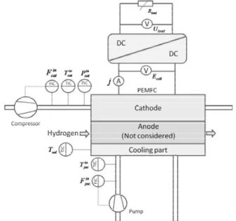
In order to use the EKF on the state estimation in a PEMFC system, a simple model should be considered. For this purpose, the study of Lauzze and Chmielewski (2006) [10] is chosen. Fig. 3 shows the piping and instrumentation
diagram (P&ID) of the selected PEM fuel cell system considered in [10]. The system consists of a fuel cell stack, air
supply sub-system, cooling sub-system and electrical devices. The fuel cell stack consists of cathode, MEA (Membrane Electrode Assemble), anode and cooling part. The air supply sub-system mainly contains a compressor which is used to feed the air into the stack. The cooling sub-system is composed of a pump which is used to feed the coolant into the stack. For the sake of simplicity, other peripheral components (e.g. radiator, back-pressure valve, heat exchanger and humidifier) are ideally treated and not displayed in the Fig. 3.
In the work of Lauzze and Chmielewski, the PEM fuel cell is treated as a CSTR (Continuous Stirred Tank Reactor) with lumped parameters. The following general assumptions are made: (1) The generated water in the fuel cell is in gas phase. (2) All gases obey the ideal gas law. (3) The temperature of all the solid materials and the coolant in the jacket is lumped. (4) The anode part is not considered in the model due to the assumption of a pure hydrogen feed.(5) The water transport in the membrane is neglected.(6) The dynamics of air stream and coolant delivery are neglected as well.
The formulated model bases on material and energy balances [10]. The material balance equations are developed
Fig. 3. P&ID of the selected PEM fuel cell system according to the work of Lauzze and Chmielewski (2006)[10]: 'A' and 'V' represent the current sensor and voltage sensor, respectively. 'FIC' means the flow indicating controller, 'TIC' the temperature indicating controller, and 'PIC' the pressure indicating
controller.
0 5 10 15 20 25 30 35 40
-1 0 1
time t
x1
0 5 10 15 20 25 30 35 40
-2 0 2 4
time t
x2
model state EKF
model state EKF
for the oxygen, nitrogen and water vapor concentrations in the cathode gas chamber. The energy balance equations are developed for the cathode gas chamber, for the solid material and for cooling part to derive the temperature in each compartment. The electrochemical kinetics are modeled by using Tafel equation. The oxygen transport from chamber to the reaction zone is modeled by Fickean diffusion equation. The oxygen diffusion coefficient is a function of relative humidity (RH) at the cathode side in order to consider flooding issues. As for the ohmic losses in the membrane, an empirical relationship between the proton conductivity, water content and temperature is employed from [11].
B. Implementation of the EKF
According to the selected model,the state vector
x
is2 2 2
[CH OCO CN TcatTsolTjac]T , which represents vapor concentration, oxygen concentration, nitrogen concentration, the temperature of the gas stream in cathode side, cell temperature and coolant temperature, respectively. In the output vectory[ucell TcatTjac p]T ,the cell voltage, the temperature of the gas stream in cathode side, coolant temperature, and total gas pressure in cathode side are included. They are measured directly by the corresponding sensors. Depending on the measurable
T
cat andp
in output vector, the total concentration of the gas in cathode can be calculated through the ideal gas law. Hence, in order to access all the six states, a vector containing the states to be estimated2 2
ˆ ˆ ˆ
ˆ [ H O O sol]T
x C C T is chosen.
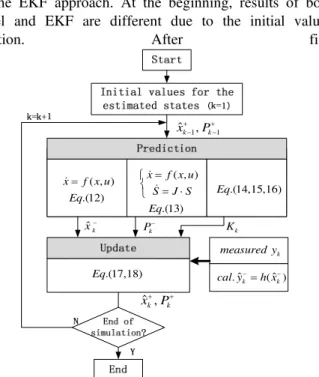
In this study, the EKF is implemented in Matlab environment. The EKF algorithm is programmed subject to the flow chart in Fig. 4. Herein, the program starts with the given initial values for the states to be estimated. Afterwards, the pre-mentioned ‘prediction step’ is executed to calculate the
x
ˆ
k by (12),P
k by (13) and Kalman gainK
k by (14)-(16). It is known that the value ofx
is critical for
P
k and can be calculated by the sensitive equation. As discussed before, a Jacobian matrix of the system model is needed. In the next, the ‘update step’ is programmed to renovate the predicted states
x
ˆ
kand covariance matrixP
kat the current sampling time. Finally, the updatedx
ˆ
k andP
k (i.e.x
ˆ
k andk
P
) will be fed into the next prediction step as new initial values, if the end condition of the simulation is not fulfilled. Such procedure is executed iteratively in Matlab.C. Simulation results
In order to test the EKF for the state estimation in the PEMFC, the related simulation is carried out. In the simulation, the current density is applied as the system input, and its profile is given in Fig. 5. It contains two step-change at t=10 s and t=20s, respectively.
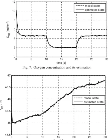
Fig. 6 and Fig. 7 show the simulated results of vapor and oxygen concentrations and theirs estimations. The dashed line represents the profile of the concentration which is calculated via the model, the solid line is the estimated profile
via the EKF approach. At the beginning, results of both model and EKF are different due to the initial values
selection. After five
seconds around, the results of EKF generally converge to the model results due to the EKF algorithm. Fig. 8 shows the simulated results of cell temperature and its estimation. It is
observed that the convergence time of cell temperature estimation is shorter than the other two states, around one second.
( , ) .(12)
x f x u Eq
( , )
.(13)
x f x u
S J S
Eq
Eq.(14,15,16)
.(17,18)
Eq
k measured y
ˆ ˆ . k ( k)
cal yh x
1 1
ˆk , k
x P
ˆk
x Pk Kk
ˆ ,k k
x P
Fig. 4. The flow chart for EKF algorithm implementation
0 5 10 15 20 25 30 2
4 6 8 10 12 14
time [s]
CH2
O
[
m
o
l/m
3]
model state estimated state
Fig. 6. Vapor concentration and its estimation
0 5 10 15 20 25 30 1000
1500 2000 2500 3000
time [s]
c
u
rr
e
n
t d
e
n
s
it
y
[A/m
2]
IV. CONCLUSION
In this paper, the principle of the EKF is introduced and illustrated by the example of the Van der Pol oscillator. The calculation of
1
ˆk
x
x
is obtained by employing the sensitive equations. Afterwards, a PEM fuel cell system is chosen. The state estimations of three internal states are selected to be estimated via the EKF. During the implementation of the EKF, the sensitive equations are employed, resulting in no requirement of model discretization. The simulation results show that the estimated states track the model results with a satisfactory manner. The implementation of the EKF in the PEMFC in this paper can be used for the purpose of system control and monitoring. It can also be migrated to other nonlinear cases after the proper modifications.
REFERENCES
[1]M. Norgaard, N. K. Poulsen, O. Ravn, New developments in state estimation for nonlinear systems, Automatica, 2000, 36, pp. 1627-1638 [2]D. Simon, Kalman filtering with state constraints: A survey of linear and
nonlinear algorithms, IET control theory and application, 2009
[3]R. Kandepu, B. Foss, L. Imsland, Applying the unscented Kalman filter for nonlinear state estimation, Journal of process control, 2007, 18(7-8) , pp. 753-768
[4]E. L. Haseltine, J. B. Rawlings, Critical evaluation of extended Kalman filtering and moving-horizon estimation, Industrial & Engineering Chemistry Research, 2005, 44, pp. 2451-2460
[5]R. K. Mandela, R. Rengaswamy, S. Narasimhan, L. N. Sridhar, Recursive state estimation techniques for nonlinear differential algebraic systems, Chemical engineering science, 2010, 65, pp. 4548-4556
[6]M. Groetsch, M. Mangold, Min Sheng, Achim Kienle, State estimation of a molten carbonate fuel cell by an extended Kalman filter, 16th European symposium on computer aided process engineering and 9th international symposium on process systems engineering, 2006, pp. 1161-1166
[7]R. Kandepu, B. Huang, L. Imsland, B. Foss, Comparative study of state estimation of fuel cell hybrid system using UKF and EKF, IEEE 2007 control and automation conference, 2007, pp. 1162-1167
[8]G.E.Suares, K.A.Kosanovich, Parameter and state estimation of a proton-exchange membrane fuel cell using sequential quadratic programming, Industrial & Engineering Chemistry Research, 1997, 36, pp. 4264-4272
[9]H. Goerguen, M. Arcak, F. Barbir, An algorithm for estimation of membrane water content in PEM fuel cells, Journal of power sources, 2006, 157, pp. 389-394
[10] K. C. Lauzze and D. J. Chmielewski, Power control of a polymer electrolyte membrane fuel cell, Industrial & engineering chemistry research, 2006, 45, pp. 4661-4670
[11] T. Springer, T. Zawodzinski, T. Gottesfeld, Polymer electrolyte fuel cell model, Journal of the electrochemical society, 1991, 138(8), pp. 2334-2342
0 5 10 15 20 25 30 0
2 4 6 8 10 12
time [s]
CO2
[m
o
l/m
3]
model state estimated state
Fig. 7. Oxygen concentration and its estimation
0 5 10 15 20 25 30 44.5
45 45.5 46 46.5 47
time [s]
Tso
l
[
oC]
model state estimated state