www.hydrol-earth-syst-sci.net/18/2521/2014/ doi:10.5194/hess-18-2521-2014
© Author(s) 2014. CC Attribution 3.0 License.
Kalman filters for assimilating near-surface observations into the
Richards equation – Part 2: A dual filter approach for simultaneous
retrieval of states and parameters
H. Medina1, N. Romano2, and G. B. Chirico2
1Department of Basic Sciences, Agrarian University of Havana, Havana, Cuba
2Department of Agricultural Engineering, University of Naples Federico II, Naples, Italy
Correspondence to:G. B. Chirico ([email protected])
Received: 3 November 2012 – Published in Hydrol. Earth Syst. Sci. Discuss.: 3 December 2012 Revised: 5 June 2014 – Accepted: 15 June 2014 – Published: 4 July 2014
Abstract.This study presents a dual Kalman filter (DSUKF – dual standard-unscented Kalman filter) for retrieving states and parameters controlling the soil water dynamics in a ho-mogeneous soil column, by assimilating near-surface state observations. The DSUKF couples a standard Kalman fil-ter for retrieving the states of a linear solver of the Richards equation, and an unscented Kalman filter for retrieving the parameters of the soil hydraulic functions, which are de-fined according to the van Genuchten–Mualem closed-form model. The accuracy and the computational expense of the DSUKF are compared with those of the dual ensemble Kalman filter (DEnKF) implemented with a nonlinear solver of the Richards equation. Both the DSUKF and the DEnKF are applied with two alternative state-space formulations of the Richards equation, respectively differentiated by the type of variable employed for representing the states: either the soil water content (θ) or the soil water matric pressure head (h). The comparison analyses are conducted with reference to synthetic time series of the true states, noise corrupted ob-servations, and synthetic time series of the meteorological forcing. The performance of the retrieval algorithms are ex-amined accounting for the effects exerted on the output by the input parameters, the observation depth and assimilation fre-quency, as well as by the relationship between retrieved states and assimilated variables. The uncertainty of the states re-trieved with DSUKF is considerably reduced, for any initial wrong parameterization, with similar accuracy but less com-putational effort than the DEnKF, when this is implemented with ensembles of 25 members. For ensemble sizes of the same order of those involved in the DSUKF, the DEnKF fails
to provide reliable posterior estimates of states and parame-ters. The retrieval performance of the soil hydraulic param-eters is strongly affected by several factors, such as the ini-tial guess of the unknown parameters, the wet or dry range of the retrieved states, the boundary conditions, as well as the form (h-based orθ-based) of the state-space formulation. Several analyses are reported to show that the identifiabil-ity of the saturated hydraulic conductividentifiabil-ity is hindered by the strong correlation with other parameters of the soil hydraulic functions defined according to the van Genuchten–Mualem closed-form model.
1 Introduction
Accurate determination of the water dynamics in the vadose zone is crucial for the success of many hydrological, cli-matic and environmental studies. The significant increase in the availability of hydrologic data sets can definitely provide extensive opportunities for reducing the uncertainty associ-ated to the detection of the spatial and temporal variability of soil moisture. However, it also calls for more robust meth-ods to merge new available observations and uncertain model predictions appropriately.
current land surface modelling efforts (Zhu and Mohanty, 2004), particularly because hydraulic properties exhibit large spatial variability at all scales of interest, making it extremely difficult to capture hydrological behaviour at one particular scale (Pringle et al., 2007; Chirico et al., 2010).
A prerequisite to properly handle the marked variability of soil hydraulic properties in large-scale applications is the use of efficient calibration methods in terms of time and stor-age. Traditional methods for parameter identification gener-ally optimize an objective function from a historical batch of data, and hence require a set of historical data to be kept in storage and processed all together, with limited flexibility to account for new available measurements (Moradkhani et al., 2005). In addition, a common problem with most of these tra-ditional inverse methods is stability and convergence (Yeh, 1986; Abbaspour et al., 1997). Therefore, several attempts have been made to develop and apply calibration methods that circumvent these drawbacks.
Considerable progress has been achieved in the develop-ment and application of sequential data assimilation (DA) techniques. As recursive data-processing algorithms, DA methods do not require all past information to be stored; they continuously update the variables under scrutiny in the model, when new measurements become available, to im-prove the model forecast and evaluate the forecast accuracy (McLaughlin, 2002; Vrugt et al., 2005; Reichle, 2008). Al-though sequential estimation is typically applied only to the state variables, some algorithms, belonging to the family of the dual estimation methods, have been designed to simulta-neously estimate model states and parameters as part of the assimilation process. This family of algorithms includes joint and dual filtering as well as expectation maximization (EM) approaches (e.g. Moradkhani et al., 2005; Liu and Gupta, 2007). EM methods have been commonly designed for off-line applications, but sequential EM methods have also been proposed (Wan and Nelson, 2001).
In the dual filtering approach, a separate state-space repre-sentation is used for the states and the parameters, while in the joint approach the unknown system states and parameters are concatenated into a single higher-dimensional joint state vector. In principle, the joint approach should provide better estimates than the dual approach, because it explicitly ac-counts for the cross-covariance between state and parameter estimates. However, the estimation process can lead to un-stable results because of complex interactions between states and parameters in nonlinear dynamic systems (Moradkhani et al., 2005; Liu and Gupta, 2007).
Some modern approaches extend the traditional parameter estimation paradigm toward a more explicit incorporation of structural data errors. Since the performance in hydrological modelling is also affected by errors in model structure and in-put data, model adjustment through time variation of param-eters together with state variables can result in a limited un-derstanding about the overall uncertainty (Clark and Vrugt, 2006). Nevertheless, the diagnostic analysis of a model can
be a difficult task and it is only possible after the model has been parameterized (Spaaks and Bouten, 2013). According to Renard et al. (2010), none of the current approaches ap-pears entirely satisfactory and the optimal methodology for handling structural errors is still to be established.
Common sequential DA methods are based on stan-dard Kalman filtering (SKF), from the innovative work of Kalman (1960). SKF became a widely used technique to merge information optimally from different sources and model predictions in linear systems (e.g. McLaughlin, 2002; Vereecken et al., 2008). Variations of the SKF algorithm have been developed to make it applicable to the sequential prob-abilistic inference problem within nonlinear dynamic sys-tems, such as the extended Kalman filter (EKF) (Jazwinski, 1970), the commonly used ensemble Kalman filter (EnKF) (Evensen, 1994, 2003), and the unscented Kalman filter (UKF) (Julier et al., 1995; van de Merwe, 2004).
A fundamental difference between the Kalman filter and variational methods is that the former explicitly evolves the covariance matrix without interruption, while variational methods do not propagate error covariance information from one assimilation interval to the next (Reichle, 2008). In ad-dition, the Kalman filter provides an analytical solution of the a posteriori state mean, while variational methods rely on numerical methods, which are considered more feasible for applications where the dimension of the state vector is very large, as with weather forecasting models (Reichle, 2008).
Kalman filter applications in hydrology (Reichle et al., 2002; Reichle and Koster, 2003; Reichle, 2008; Camporese et al., 2009) favour the use of EnKF, relying on the propa-gation of a random ensemble of the retrieving variable. The EnKF is an advantageous approach for highly dimensional applications, mainly because, by means of a comparably small ensemble of model trajectories, it captures the relevant parts of the error structure (Reichle, 2008). This method also facilitates the treatment of errors in model dynamics and pa-rameters (Reichle and Koster, 2003; Moradkhani et al., 2005) and it is easily scalable. Nevertheless, the EnKF estimation based on small ensemble sizes, can be affected by spurious modes and large biases even if the ensemble mean and co-variance are correct (Luo and Moroz, 2009; Lei and Baehr, 2013). Moreover, the optimal ensemble size for the EnKF is uncertain and is generally chosen on the basis of a heuristic evaluation.
The sampling strategy of the EnKF could be a drawback in large-scale applications where a small variation of the en-semble size has an important impact on the computational demand (e.g. Kumar et al., 2008). The implementation of these large-scale assimilation systems is often described as a collection of independent low dimensional assimilation problems (Crow and Wood, 2003; Reichle and Koster, 2003; Kumar et al., 2008).
retrieval performances similar to those obtained with non-linear schemes, but with less computational effort, also cir-cumventing some issues which may arise with the sampling strategies used by the UKF and the EnKF. However, the UKF can be more flexible and computationally efficient than the EnKF in problems with low degrees of freedom, because it relies on ensemble sizes equal to twice the number of degrees of freedom plus one.
Few attempts have been made to retrieve soil water state profiles and soil hydraulic parameters simultaneously by as-similating near-surface observations with Kalman filters (e.g. Qin et al., 2009; Yang et al., 2009; Montzka et al., 2011). Tian et al. (2008) used a dual UKF for reproducing the temporal evolution of daily soil moisture under freezing conditions by assimilating satellite observations. Lü et al. (2011) developed a dual Kalman filter for estimating the root zone soil moisture using a model based on the Richards equation, by combining the EKF to update the state variables, with an optimization al-gorithm for retrieving parameters of soil hydraulic functions defined according to the van Genuchten–Mualem (VGM) re-lations (van Genuchten, 1980). Monztka et al. (2011) per-formed a joint approach retrieving soil moisture and VGM parameters, but using a particle filter algorithm.
Moving from the result of Chirico et al. (2014), we hy-pothesize that the combination of SKF applied to a linearized numerical representation of the Richards equation, and UKF applied to handle the intrinsic nonlinearities between hy-draulic parameters and soil water states, could provide a suitable strategy for optimizing the prediction of the state dynamics.
The first objective of this study is to illustrate the feasibil-ity of using a deterministic dual filter approach to perform simultaneous retrieval of soil moisture profiles and VGM pa-rameters, with similar accuracy but reduced computational expense, as compared with ensemble Kalman filters, based on the assimilation of near-surface observations in a one-dimensional Richards’ equation. The analysis is based on a synthetic test assuming uncertain observations and a poor guess of the initial states. A small structural error is also in-volved by implementing a different numerical solver of the Richards equation in the assimilation algorithm from that employed for generating the reference synthetic data.
The dual Kalman filter (hereafter referred to as DSUKF – dual standard-unscented Kalman filter) is designed by cou-pling the SKF approach for retrieving the states with the UKF for retrieving soil hydraulic parameters. For compara-tive purposes, the simultaneous retrieval of states and param-eters is also performed using the dual ensemble Kalman fil-ter (DEnKF), following the framework described by Morad-khani et al. (2005). Interested readers are referred to this work, widely cited by the hydrological data assimilation community.
A second objective is to compare the potential advan-tages and limitations of anh-based or aθ-based form of the Richards equation in the retrieval algorithm, also
account-ing for different initial guesses of the parameters, observa-tion depths, assimilaobserva-tion frequencies as well as the type of near-surface observations (horθ).
2 Model and methods 2.1 Governing equation
As in the vast majority of applications in this realm, we de-scribe the vertical movement of water under isothermal con-ditions in a rigid, homogeneous, variably saturated porous medium using the Richards equation (Jury et al., 1991). The following two equations represent the Richards equation in theh-based and inθ-based forms, respectively:
∂θ
∂t =C (h) ∂h
∂t =
∂hK (h)∂h∂z−1i
∂z , (1)
∂θ ∂t =
∂hD (θ )∂θ∂z−K (θ )i
∂z , (2)
wheretis time andzis soil depth taken as positive downward withz=0 at the top of the profile,C (h)= dθ/dh[1/L] is the specific water capacity of the soil at matric pressure head,
h, obtained by differentiating the functionθ (h), andD (θ )=
K (θ )/C (θ )[L2/T] represents the unsaturated diffusivity. For an efficient numerical solution of the model, it is con-venient to describe the soil hydraulic properties using closed-form analytical relationships. The following non-hysteretic VGM equations (van Genuchten, 1980) are widely used in soil hydrology:
θ (h)=θr+(θs−θr)1+ |αh|n−
m
, (3)
K (θ )=KsSeλ h
1−1−S1e/m mi2
, (4)
whereθs is the saturated soil water content,θr is the resid-ual soil water content,Se=(θ−θr)/(θs−θr)is the effective saturation,Ksis the saturated hydraulic conductivity, andα [L−1],n(-),m(-) andλ(-) are empirical scale and shape pa-rameters. A common assumption, also adopted in this work, is to setλ=0.5 and posem=1−1/n.
2.2 Numerical formulation of the model
Chirico et al. (2014) showed that the implementation of the filtering approach upon a linearized Crank–Nicolson finite difference scheme (CN) can be an efficient algorithm for one-dimensional problems. The differentiation of Eq. (1) for in-termediate nodes according to the CN scheme, leads to the expression
−Kki−−11/2
21zi1zu; Cki−1 1tk−1+
Kki−−11/2 1zu +
Kki+−11/2 1zl 21zi ;
−Kki+−11/2
21zi1zl
hik−1 hik hik+1
=
Kki−−11/2
21zi1zu; Cki−1 1tk−1−
Kki−−11/2 1zu +
Kki+−11/2 1zl 21zi ;
Kki+−11/2
21zi1zl
hik−−11 hik−1 hik+−11
+
Kki−−11−Kki+−11
21zi , (5)
where superscript i is the node number (increasing down-ward), subscriptkis the time level, and1tk=tk+1−tk. The
soil column is divided into compartments of thickness1zi. All nodes, including the top and bottom node, are in the centre of the soil compartments, with 1zu=zi−zi−1and
1zl=zi+1−zi. The spatial averages ofKare calculated as arithmetic means.
Assuming flux boundary conditions, the differential equa-tions at the top and bottom nodes respectively are
Ck1−1 1tk−1+
K1
1 2
k−1 21z11zl;
−K1
1 2
k−1
1z11zl
h1k h2k
(6)
=
Ck1−1 1tk−1−
K1
1 2
k−1 21z11zl;
K1
1 2
k−1
1z11zl
h1k−1 h2k−1
+qtop−K 112
k−1
1z1 ,
−KkN−−11/2 1zN1zu ;
CkN−1 1tk−1+
KkN−−11/2
21zN1zu !
hNk−1 hNk
(7)
= K
N−1/2
k−1 21zN1zu;
CkN−1 1tk−1−
KkN−−11/2
21zN1zu
!
hNk−−11 hNk−1
+K
N−1/2
k−1 −qbot
1zN ,
whereqtopandqbotare the fluxes at the top and bottom of the soil profile, respectively.
The analogous differential expressions of the Richards equation in theθform (Eq. 2) can be obtained from Eqs. (5)– (7) by simply removing the soil water capacity (C)and by substitutinghwithθ, the hydraulic conductivity (K)of the dependent terms with the diffusivity (D), while keeping the independent terms on the right-hand side unchanged.
In the numerical scheme, the explicit linearization of K
andC(orD)is implemented by taking their values at the pre-vious time stepk−1. A linear state-space representation of the dynamic system can then be easily derived by combining
the set of Eqs. (5)–(7) written for each node and accounting for the boundary conditions:
Bk−1xk=Ak−1xk−1+fk−1, (8) wherexrepresents the state vector (i.e. either soil water con-tents or matric heads in the soil profile), whileAk−1andBk−1 are tridiagonal matrices obtained by assembling the terms in the first parenthesis on the right- and left-hand side of Eqs. (5)–(7), respectively. The termfk−1is a vector obtained by assembling the terms on the right-hand side of the state variable at time stepk−1. More explicitly, Eq. (8) becomes
xk=Fk−1xk−1+gk−1, (9)
whereF=B−1Aandg=B−1f.
2.3 The dual standard-unscented Kalman filter (DSUKF) formulation
The dual filter approach has been implemented with most of the variants of the Kalman filter, applied to both linear and nonlinear problems, i.e. the SKF (Todini et al., 1976), the EKF (Nelson, 2000; Wan and Nelson, 2001), the EnKF (Moradkhani et al., 2005) and the UKF (Wan and van der Merwe, 2001; van der Merwe, 2004).
In this section we illustrate the (DSUKF) formulation, where the SKF is implemented for retrieving the states of a linear system, while the UKF is applied to handle the marked nonlinearities between states and parameters.
At every time stepk, the posterior parameter estimate at timek−1 is used in the state filter, while the current estimate of the states is used in the parameter filter. In the most general case, the set of system equations for the states can be written as follows:
xk=Fk−1,k xk−1,uk,wˆk−1+νk−1, (10)
yk=Hk xk,wˆk−1+ηk. (11)
In a Bayesian framework, they represent a prior distribution over the states. Equation (10) allows inferring the transition probability density of the states, while Eq. (11) determines the probability density of the observations given the prior states. The set of system equations for the parameters can be written as
wk=wk−1+ξk−1, (12)
yk=Hk Fk−1,k xˆk−1,uk,wk,wk+ςk, (13)
representing a prior distribution over an artificial time-dependent random variable that emulates model parameters. In the equations above,ukis the exogenous input assumed
to be known at instant tk; νk−1 accounts for a simplified representation of the model errors, assumed to be a zero-mean Gaussian process noise with covarianceQk−1, while
ηk is the zero mean and temporally uncorrelated
the observation of the states. The state transition density
p (xk|xk−1,uk,wk−1)is fully specified byFk−1,k and the
process noise distributionp(νk−1), whereasHk and the
ob-servation noise distributionp(ηk)fully specify the
observa-tion likelihoodp(yk|xk,wk).
Fk−1,k andHkare parameterized via the parameter vector wk, whose evolution is artificially set up in a way similar
to that employed for the state variables (Moradkhani et al., 2005) by means of a stationary process with identity state transition matrix.ξk−1∈N 0,Qw,k−1
is the noise driving parameter updating, andςk=ηk+ξkis the noise corrupting the observation equation relative to the parameters, with zero mean and covariance Rw,k. The upper symbol “ˆ” denotes
the density mean of the variable.
2.3.1 UKF algorithm for parameter retrieval
The UKF, like the EnKF, is based on a strategy for the selec-tion of the sample points, which aims to capture the poste-rior true mean and covariance of the retrieved variable, after the sample points are propagated through the true nonlinear system. States or parameters are still represented by a Gaus-sian random variable. However, in the UKF this is not spec-ified by an ensemble of randomly chosen points, like in the EnKF, rather by using a minimal set of deterministically cho-sen sample points.
Consideringwˆ andPw, respectively, as mean and
covari-ance of the parameter vectorwto be retrieved, having the di-mension equal toNpar, the UKF selects a set of sigma points Si=µi,Wi, i=0. . .2Npar , consisting of 2Npar+1 vec-torsWiand their associated weightsµi, completely
captur-ing the actual mean and covariance of the random variable
w. A selection of sigma points fulfilling this requirement is defined as follows:
W0= ˆw;Wi= ˆw+ p
γPw
i, i=1, . . ., Npar;Wi
= ˆw−pγPw
i, i=Npar+1, . . .,2Npar, (14) µ(m)0 =γ−Npar
γ ;µ
(c)
0 =
γ−Npar
γ +
1−ρ2+β;µ(m)i
=µ(c)i = 1
2(γ ), i=1, . . .,2Npar. (15)
Weight values for calculating the mean and the covariance are distinguished by the upper indexes m and c, respec-tively. The other parameters are defined as follows: γ= ρ2 Npar+κ, whereρis a factor employed to expand or to shrink the sample state distribution around the mean; κ is a scaling parameter;β affects the weights of the points when calculating the covariance. Details about the proper choice of
ρ,βandκcan be found in the work of van der Merwe (2004). The term √γPwi is the ith column (or row) of the root
square matrix γPw, calculated by Cholesky decomposition
(Press et al., 1992).
The evolution of the parameter mean and covariance dur-ing each time step is computed as follows
ˆ
w−k = ˆwk−1 (16)
P−w,k=Pw,k−1+Qw,k−1. (17) The artificial noise covarianceQw is computed as follows
(Wan and Nelson, 1997; Nelson, 2000; van der Merwe, 2004):
Qw,k=
λ−RLS1 −1Pw,k. (18)
The parameterλRLS∈(0,1] is considered a forgetting fac-tor, as defined in the recursive least-squares (RLS) algorithm. Nelson (2000) showed that settingλRLS<1 (i.e. the prior co-variance is larger than the posterior coco-variance) provides an approximate exponentially decaying weight on past data. By settingλRLS=1 (i.e. no process noise for the parameters is considered) all past data are equally weighted to obtain the current dynamics.
Whenever measurements are available, new sample states are created by substituting the a priori parameter mean,wˆ−k, and covariance,P−w,k, in Eq. (14). In principle the weights,
µi, do not change during the simulation.
The set of 2Npar+1 parameter vectorsWk is propagated
across the model, and the observation equation, using as states the a posteriori mean atk−1,xˆk−1, is expressed as
follows:
Yk=Hk Fk−1,k xˆk−1,uk,vk−1,Wk. (19) Yk also represents a set of 2Npar+1 vectors, each having
Nobselements.
The Kalman gain employed for modifying the parameter trajectories is obtained as follows:
Kw,k=Pwy,k
Pwyy,k+Rw,k −1
=Pwy,k Pwυυ,k −1
. (20) Pwy,kis computed by the following weighted outer product:
Pwy,k=
2Npar
X
i=0
µ(c)i Wk,i− ˆw−k
Yk,i− ˆy−w,k T
. (21)
ˆ
y−w,k is a weighted average of the predicted measurements
Yk,i:
ˆ
y−w,k=
2Npar
X
i=0
µ(m)i Yk,i. (22)
Pwyy,kis given by
Pwyy,k= 2Npar
X
i=0
µ(c)i Yi,k− ˆy−w,k Yi,k− ˆy−w,k T
The measurement noise covarianceRw,k is assumed to be a
constant diagonal matrix following the basic implementation of the dual UKF proposed by van der Merwe (2004), previ-ously applied by Wan and Nelson (1997), Nelson (2000) and Wan and Nelson (2001) in the context of a dual EKF. This as-sumption leads to a recursive prediction error algorithm that minimizes a simplified cost function with respect to the pa-rameters. This prediction error algorithm, while questionable from a theoretical perspective, has been shown to be quite useful (Wan and Nelson, 2001). As part of a dual UKF ap-plication, Gove and Hollinger (2006) showed that by setting the measurement noise covariance equal to the identity ma-trix, the overall trajectory of the retrieved parameter was very similar to that obtained considering the actual measurement errors, and attributed this behaviour to the robustness of the filter with respect to changes in parameter measurement vari-ance components.
The parameter mean is updated according to the standard Kalman filter equation:
ˆ
wk= ˆw−k−1+Kw,k
yk− ˆy−w,k
. (24)
The parameter covariance is updated as follows:
Pw,k=P−w,k−Kw,kPwυυ,k Kw,kT. (25)
Pwυυ,k(see also Eq. 19) represents the covariance ofyk− ˆy−w,k.
Here we opt for the expression also employed by Julier and Uhlmann (2004), van der Merwe (2004) and Tian et al. (2008), given the nonlinearity between parameters and ob-servations.
2.4 Algorithm for parameter sampling
Given the marked differences in the range of variation of the VGM parameters, a variable transformation is required to guarantee operational stability. Bounding parameters by means of a function of reference values and a variable cor-rection term ensures that the model behaves reliably. Morad-khani et al. (2005) and Montzka et al. (2011) also applied some strategies to limit the overdispersion of parameter sampling.
Given thatwiis the true value of theith parameter, the
pa-rameter estimation system makes use of the following vari-able transformation:
wi =wimin+ wimax−wiming(δwi), (26) wherewminandwmaxrepresent user-defined nominal values, indicating the minimum and maximum values of the param-eter, respectively, while the correction term, δw, which is the actual variable under estimation, is expressed as an inde-pendent term of a nonlinear sigmoidal functiong(δw). This function g(δw), termed a “squashing function” by van der Merwe (2004), limits the absolute magnitude of iterative pa-rameter adjustment, further preventing the divergence of the
parameter estimations. Therefore, the parameters are not es-timated directly, rather “correction terms” are eses-timated.
A preliminary analysis has shown that the approach is not very sensitive to the type of sigmoidal function and that the following relationship performed well for all of the circum-stances examined:
g(δwi)=
δwi
2(1+ |δwi|)+
0.5. (27)
Note that lim
δwi→−∞
g(δwi)=0 and lim
δwi→∞
g(δwi)=1, in which caseswi=wiminandwi =wimax, respectively.
3 Synthetic experimental framework
We explore the performance of the proposed dual Kalman fil-ter with a synthetic study. The main advantage of testing the algorithm with a synthetic study is that, by knowing the true system, the results are not overshadowed by other sources of uncertainty: a fundamental aspect that should be addressed prior to evaluating algorithm performance with real data, as in the study presented by Medina et al. (2014).
3.1 Model implementation and synthetic data generation
We simulate the vertical movement of water in a homoge-neous and variably saturated soil column of 100 cm. The hy-draulic properties of the homogeneous soil column are iden-tified by using the VGM parameters reported in the papers by Entekhabi et al. (1994) and Walker et al. (2001):θsT=
0.54; θrT =0.2; KsT=0.00029 cm s−
1, α
T=0.008 cm−1 andnT=1.8, where the subscript “T” indicates the “true” values, i.e. those employed to produce the reference syn-thetic simulations. However, different boundary conditions have been set so as to make the synthetic study more repre-sentative from a practical perspective:
– the top boundary condition is the result of a combination of a stochastically generated daily series of rainfall plus a constant evaporation rate of 2.35 mm d−1;
– the bottom boundary condition is set by a zero gradient of the matric head, also known as “free drainage” con-dition, which also implies that this condition is affected by uncertainty in the identification of the unsaturated hydraulic conductivities.
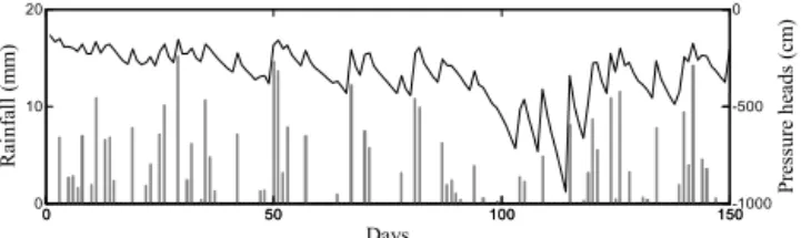
0 50 100 150 0
10 20
Days
R
ainf
all (
m
m
)
0 50 100 150-1000
-500 0
Pres
su
re h
ea
d
s
(c
m
)
Figure 1. Rainfall pattern (bar plot) and synthetically generated “true” matric pressure head values at 5 cm depth (solid line).
than the case with a constant top boundary condition, which is the one applied by Entekhabi et al. (1994) and Walker et al. (2001).
Daily rainfall is obtained by stochastically sampling a Poisson probability distribution of the occurrence of daily events with an exponential distribution of the rainfall depth. The bar plot in Fig. 1 illustrates the synthetic daily rainfall time series for a period of 150 days.
The soil column is discretized by 27 nodes with variable node spacing; this according to van Dam’s (2000) sugges-tion that accurate computasugges-tion of soil water fluxes at the top boundary requires that the distance between the nodes close to the soil surface has to be in the order of a few centimetres. A similar criterion is followed for the bottom compartments, given the flux condition adopted for the bottom boundary.
Subsequently, time series of synthetic “true” matric head and soil moisture profiles are generated for 150 days, by setting the initial profile matric head uniformly equal to −50 cm, and by employing the nonlinear numerical scheme illustrated by Chirico et al. (2014). Figure 1 also shows the time series of the generated matric pressure head values at 5 cm depth.
3.2 Retrieval modes
The synthetic study involves the retrieval of states and parameters by assimilating near-surface observations into the Richards equation, according to three different retrieval modes:
– the h-h retrieval mode, indicating that matric head is used as both observed and state variable, with the h -based form of the Richards equation;
– theθ-θretrieval mode, indicating that soil water content is used as both the observed and state variable, with the
θ-based form of the Richards equation;
– theθ-hretrieval mode, indicating that soil water content is used as the observed variable, while matric head is used as the state variable, with theh-based form of the Richards equation.
Preliminary analyses showed that the h-h mode is prone to volatility in the parameter solution, for relatively abrupt changes in the original state variable, generating either very
large or very small values. When the solution is very close to the extreme values, the parameter estimation filter some-times loses its tracking ability, and the algorithm becomes unstable.
A successful strategy is to work with log transformed ma-tric heads only for the parameter filter, without the need to make any change in state relationships. This alternative can be implemented straightforwardly in a nonlinear KF as UKF or EnKF, where the covariance matrices are not propagated analytically. Hence, in theh-hmode the parameter equations are not directly applied with log transformed predicted mea-surements and observations.
As illustrated below, the retrieval algorithm using soil moisture as a state variable is permanently stable, albeit at the expense of a slightly slower convergence speed, as compared with the case ofhas a state variable. As stated by Walker et al. (2001), the soil moisture transformation not only reduces the differences between model predictions and observations, but also the numerical values of the gradients along the soil profile.
3.3 Reference scenarios
The performance of the proposed dual Kalman filter ap-proach is evaluated with respect to reference scenarios, given by implementing the three retrieval modes introduced in the previous section, with different assimilation depths, assimi-lation frequencies and initial guessed parameter sets.
We simulate the assimilation of observed variables at three alternative observation depths (OD): 2, 5 and 10 cm. Escori-huela et al. (2010) found 2 cm to be the most effective soil moisture sampling depth by L-band radiometry. Neverthe-less, L-band sensors receive their signal from approximately the top 5 cm, on average (Kerr, 2007). A depth of 10 cm rep-resents the maximum observation depth that can probably be explored with the current remote sensing technology (e.g. Nichols et al., 2011).
We also examine three alternative assimilation frequencies (AF): 1, 1/3 and 1/5 d−1. Daily assimilation frequency ac-counts for future L-band missions or a combination of differ-ent remote sensors, whilst 3 days is the minimum time inter-val of SMOS spaceborne platforms (Kerr et al., 2010). One observation every 5 days represents a more common remote sensing time frequency.
The assimilation scenarios with theh-based form of the Richards equation are initialized with an initial matric pres-sure head profile assumed to be uniformly equal to−100 cm. The assimilation scenarios with the θ-based form of the Richards equation are initialized with an initial soil water content profile uniformly equal to−0.47 cm3cm−3, which corresponds to the soil water content ath=−100 cm, accord-ing to the true water retention function.
methods, i.e. with pedotransfer functions (e.g. Chirico et al., 2007).
We considered six very dissimilar sets of initial values for the parametersKs,α, andn, to evaluate the role exerted by different initial guesses on the performance of the retrieval process. These initial values were identified by employing the six possible permutations of the values−1, 0 and 1 as cor-rection termsδwi in Eq. (27), and subsequently in Eq. (26).
The initial matrix of the normalized correction terms associ-ated with the soil hydraulic parameters is set to be diagonal, with non-zero entries equal to 0.01, following Nelson (2000). Table 1 shows the resulting initial values of the parameters and the correspondingwminandwmax–wmin. Notice that the limit values of our parameters, wminandwmax, cover prac-tically the whole spectrum of values reported by Carsel and Parrish (1988) for the 12 major soil textural groups, except for some sandy soils.
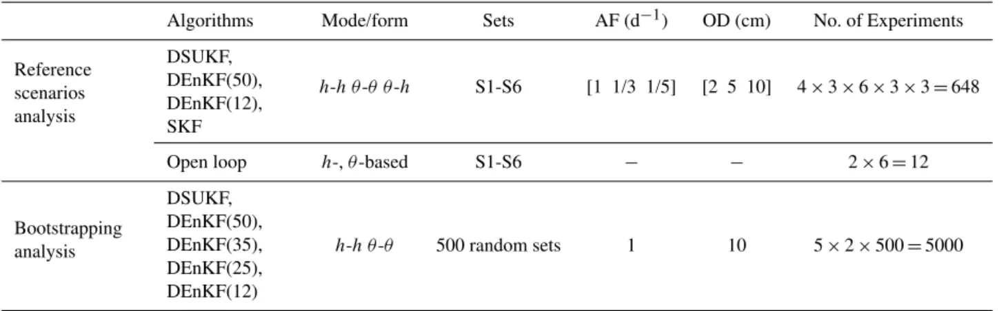
On the whole, 162 reference scenarios are examined, made by three retrieval modes, three observation depths, three as-similation frequencies and six initial parameter sets. 3.4 Comparative performance analyses
The DSUKF performance in retrieving the state profiles is analysed by comparing it with the DEnKF, the SKF and the “open loop” solution.
The DEnKF is implemented following the framework described by Moradkhani et al. (2005), coupled with the fully implicit numerical representation of the Richards equa-tion described by Chirico et al. (2014). The DEnKF is run with ensembles of 12 members (hereafter referred to as DEnKF(12)) and 50 members (hereafter referred to as DEnKF(50)). Reichle and Koster (2003) found that the un-certainty in soil moisture retrieved with an EnKF applied to a one-dimensional problem, is consistently reduced with an ensemble of 12 members. Camporese et al. (2009) suggest a minimum of about 50 realizations for ensuring a suitable level of accuracy in analogous applications.
The SKF is implemented with a linearized Crank– Nicolson finite difference scheme of the Richards equation (Chirico et al., 2014), with time-independent initial guessed parameters.
The “open loop” solution is obtained without assimilat-ing any near-surface observations, i.e. the system is simply propagated from the initial uniform conditions and the time-independent initial guessed parameters, using the known boundary conditions.
For quantitatively evaluating the performance of the re-trieval algorithms, the normalized root mean square error (RMSE) between predicted and synthetic data (SD) state pro-files is calculated as follows:
RMSEj=
1
σSD v u u t
Nnod
X
i=1
xi,jp −xi,jSD2/(Nnod−1), (28)
wherexpi,jandxi,jSDrepresent the predicted and SD state value at nodeiand timej, respectively, andσSDis the standard de-viation of the SD state series, withNnod=27. Normalization is carried out to enable the comparison betweenθ-based and
h-based retrieval processes.
The average RMSE of the last 15 days of simulation (here-after simply referred to as RMSE) is taken as accuracy index of the retrieved state profiles, since RMSE values in the last 15 days are not affected by the poor guess of the initial con-dition. Under the assumption of “free drainage” at the bottom boundary, the dynamic evolution of the system’s states, con-ditional upon a specific set of parameters, rapidly loses its dependence on the initial state values, and the effect of the poor guess of the initial state disappears after a few weeks.
The performance in state retrieval is thus analysed by com-paring the RMSE of 648 experiments, resulting from the ap-plication of four retrieval algorithms (DSUKF, DEnKF(50), DEnKF(12) and SKF) to the 162 reference scenarios out-lined in the previous section. In addition, another 12 experi-ments are undertaken for the “open loop” solutions, resulting from the application of theh-based andθ-based forms of the Richards equation with the six sets of parameters.
The reference scenarios, but only in theh-handθ-θ re-trieval modes, are also employed for assessing the capability of DSUKF to identify the unknown parameters. The effect of dealing with a nonlinear observation operator in theθ-h
mode is examined by comparing the parameters retrieved in theh-hand in theθ-hretrieval modes, but using an hourly assimilation frequency.
Further insights into parameter identifiability are gained by comparing the performances of the retrieval algorithms in estimating the states when only one or two parameters are uncertain.
Table 1.Values of the true parametersKs,αandn, the minimum,wmin, and the range,wmax–wmin, used to constrain their distribution, and
the resulting six sets of input values considered during the assimilation process.
Parameter True wmin wmax–wmin S1 S2 S3 S4 S5 S6
Ks(×10−4cm s−1) 2.9 0.1 6.0 4.6 4.6 3.1 3.1 1.6 1.6
α(×10−2cm−1) 0.8 0.1 5.0 2.6 1.35 3.85 1.35 2.6 3.85
n(–) 1.8 1.1 2.0 1.6 2.1 1.6 2.6 2.6 2.1
Table 2 provides an overview of the numerical experiments undertaken for assessing the relative performance of DUSKF. 3.5 Setting system and noise covariances
The covariance matrices of the added process and measure-ment noises (Q,Qw,RandRw)and the initial system
co-variance matrices (P0 andPw,0) are set to be diagonal for
all cases. The initial state covariance matrix accounts for a standard deviation of 32 % of the initial state value, denot-ing a sufficiently high, yet realistic, error, with no correlation between nodes. This corresponds to an initial covariance of 103cm2using theh-based form of the Richards equation and 0.023 using theθ-based form. The response to a variation of the initial system covariance in a dual Kalman filter frame-work is less predictable than in a state Kalman filter appli-cation, where an increase in the error covariance regularly drives the system to converge faster to the true regime, pro-vided that the variance of the observation error is lower.
Similarly to Camporese et al. (2009), a standard deviation of 1.4 % of the observed value was given to the observation noise, while a standard deviation of 2.24 % was given to the system noise. These values respectively correspond to a co-variance of 2 and 5 % of the initial state value in theh-based form, as also adopted by Walker et al. (2001).
The system noise covariance was added every hour as a means of normalizing the incorporated error with respect to the time step, i.e. to make the incorporated error independent of the adopted time step.
We set b=2.0 andk=0 for the deterministic sampling within the UKF (see Eq. 14), as suggested by van der Merwe (2004). The ensemble size is equal to seven, i.e. twice the number of retrieved parameters (Npar)plus one. Through sensitivity experiments, we choseρ=0.3 using theh-hand
θ-hmodes, andρ=0.8 using theθ-θmode.
The forgetting factor coefficientλRLS, affecting the artifi-cial parameter noise covarianceQw(Eq. 17), was set equal to
0.995 in theh-based form and to 0.9999 in theθ-based form, while the diagonal entries of the artificial observation noise covarianceRwwere set equal to 0.5 and 10−5, respectively.
Given that these coefficients are subjectively chosen and have a major effect on parameter updates, we also examined some scenarios accounting for different combinations ofλRLSand Rwvalues, as listed in Table 3 for both retrieval modes.
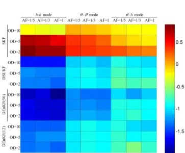
Figure 2.The colour scale indicates the logarithm of the ratio be-tween the RMSE of SKF, DSUKF, DEnKF(50) and DEnKF(12), and the corresponding RMSE of the open loop solution, for three retrieval modes (h-h,θ-θ andθ-h), three assimilation frequencies (AF=1, 1/3 and 1/5 d−1)and three observation depths (OD=2, 5 and 10 cm). RMSE values have been averaged among the six initial guessed parameters sets (S1–S6).
4 Results
4.1 State retrieval
The coloured grid depicted in Fig. 2 provides a compre-hensive representation of the relative performances of the Kalman-based retrieval algorithms with respect to the ref-erence scenarios. The colour scale indicates the logarithmic of the ratio between the RMSE of the examined assimila-tion algorithm and the RMSE of the open loop soluassimila-tion, both averaged among the six parameter sets. The average RMSE values retrieved in theh-hand in theθ-hmodes are divided by the average RMSE open loop value obtained with theh -based form. The average RMSE values retrieved in theθ
-θ mode are divided by the value obtained with theθ-based form. Thus, looking at the different retrieval modes, only the cells of the grid referring to theh-hand theθ-hmodes can be directly compared.
Table 2.Summary of numerical experiments involved in the performance analyses.
Algorithms Mode/form Sets AF (d−1) OD (cm) No. of Experiments
Reference scenarios analysis
DSUKF, DEnKF(50), DEnKF(12), SKF
h-h θ-θ θ-h S1-S6 [1 1/3 1/5] [2 5 10] 4×3×6×3×3=648
Open loop h-,θ-based S1-S6 − − 2×6=12
Bootstrapping analysis
DSUKF, DEnKF(50), DEnKF(35), DEnKF(25), DEnKF(12)
h-h θ-θ 500 random sets 1 10 5×2×500=5000
Table 3.Scenarios for assessing the effect of the artificial noise vari-ance in parameter state space equations.
h-hretrieval mode θ-θretrieval mode
Scenario λRLS Rw Scenario λRLS Rw
1 0.975 10−4 6 0.975 10−5 2 0.95 10−3 7 0.995 10−5 3 0.975 10−3 8 0.9999 10−5 4 0.999 10−3 9 0.9999 10−3 5 0.975 10−2 10 0.9999 10−4
methods improve the open loop estimations independently on the adopted scenario.
The RMSE values of the DSUKF estimations are in all cases higher than those obtained using DEnKF(50), but gen-erally lower than the ones of the DEnKF(12). The observa-tion depth and the assimilaobserva-tion frequency affect the retrieval performance of the dual filters more in theθ-θand in theθ-h
modes than in theh-hmode.
Figure 2 clearly shows that the retrieval performance with theθ-hmode is much poorer than that one obtained with the
h-hmode. This occurrence confirms that a nonlinear obser-vation operator in the θ-hmode has a relevant detrimental effect on the state-retrieving performance. Therefore, later in this section we specifically focus on the comparison of the
h-hand theθ-θretrievals, by showing additional results. Figure 3 depicts the absolute RMSE values, in the h-h
mode and the θ-θ mode, for two extreme assimilation sce-narios: one with OD=10 cm and AF=1 d−1, the other with OD=2 cm and AF=1/5 d−1. The RMSE of the open loop simulations obtained withθ-θmode is lower than those rele-vant to theh-hmode, showing the lower impact that param-eter uncertainty exerts on the soil water content uncertainty with respect to the matric head uncertainty. Although the ini-tial conditions in terms ofhorθare consistent between them according to the “true” soil water retention function, they ac-tually have a different impact on the corresponding open loop
Figure 3.Logarithm of RMSE of the state profiles computed for open loop simulations, SKF, DSUKF, DEnKF(50) and DEnKF(12), in theh-h(left column) and in theθ-θ(right column) modes.
simulation errors because of the poor guess in the parame-ters. In addition, these results may also be biased somehow because the soil moisture space is constrained, whereas the matric head space is not and it is theoretically infinite.
For OD=2 cm and AF=1/5 d−1, the RMSE is about 18 and 9 times lower than with the corresponding open loop solu-tions. The RMSE with the h-hmode is always lower than that with the θ-θ mode, except for the case with the initial parameter set S4.
The RMSEs of DSUKF are about 2.5 and 1.65 larger than using DEnKF(50), respectively for theh-hmode and theθ-θ
modes, almost irrespective of the time and space resolutions of the assimilated observation. DEnKF(50) also appears to be less vulnerable to the anomalies affecting the DSUKF al-gorithm implemented with the matric heads, but its compu-tational time is almost seven times larger than that required for DSUKF. However, with OD=10 cm and AF=1 d−1, the DSUKF errors are approximately 1.6 and 1.4 times lower, respectively, than those of DEnKF(12) .
For OD=2 cm and AF=1/5 d−1, the DEnKF(12) per-formed similarly to the DSUKF in terms of RMSE, but it is subjected to some numerical artifacts, in particular for S4, due to the relatively large sampling errors associated with the small size of the ensemble. In addition, the computational time required for DSUKF is about 1.7 times smaller than that required for DEnKF(12).
Figure 4 shows the states retrieved using theh-handθ-θ
retrieval modes after 5, 10, 20, 50, 100 and 150 days, con-sidering the minimum assimilation frequency of the near-surface observations (AF=1/5 d−1), together with the open loop profiles.
The two sets of open loop profiles simply reflect the same model predictions with two different representations of the system states, which are reciprocally related by means of the water retention function parameterized according to the cor-responding guessed parameters. Compared with the corre-sponding true profiles, the open loop matric head profiles are biased toward larger matric heads, while the open loop wa-ter content profiles are mainly shifted toward lower content values.
The DSUKF, with both retrieval modes, considerably re-duces the uncertainty of the states despite the initial wrong parameterization. At the 50th day, a good match is observed between the estimated and “true” profiles , almost irrespec-tive of the initial guessed parameter set.
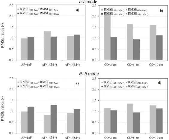
Figure 5 depicts the ratios of the mean RMSE within each group of parameter sets, computed during the last 15 days for different observation depths and assimilation frequencies. In general, the RMSE exhibits limited sensitivity to the obser-vation depths under the adopted range (Fig. 5a, c). In the case of theθ-θ retrieval mode, the ratio between OD=2 cm and OD=5 cm is even smaller than one both for AF=1/3 and AF=1/5 d−1, which should be due to the stochastic nature of the simulations. Increasing AF from 1/5 to 1/3 d−1 does not appreciably improve the error statistics. Only the tran-sition from AF=1/3 d−1to daily assimilations consistently reduces the RMSE, particularly with matric heads (Fig. 5b, d). With the DEnKF(50) (Fig. 3), the RMSE for OD=2 cm and AF=1/5 d−1, compared with that assuming OD=10 cm
and AF=1 d−1, is about 2.1 times larger with theh-hmode and 1.3 times larger with theθ-θ mode, consistent with the results obtained with the DSUKF.
The ratio of the mean RMSE computed with theθ-θ re-trieval mode to that obtained with the h-h mode is about 1.7 considering AF=1 d−1, while it is close to one for the other two frequencies. The values reported in Fig. 3 for DEnKF(50) show that the RMSE with theθ-θ mode is 2.4 times higher than with theh-h mode, for OD=10 cm and AF=1 d−1, and 1.5 times higher for OD=2 cm and AF=1/5 d−1. However, the average statistics are strongly af-fected by the high errors obtained for S4 and S5.
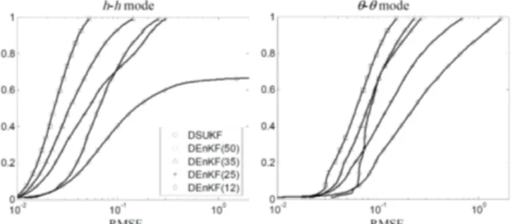
Given the stochastic nature of the problem, we examine the probabilistic distribution of the error of the estimated states by applying the DSUKF and the DEnKF with 500 random sets of initial parameters, as illustrated in Sect. 3.4. Figure 6 shows cumulative probability distributions of the RMSE ob-tained with DSUKF, DEnKF(12), DEnKF(25), DEnKF(35), DEnKF(50), assuming OD=10 cm and AF=1 d−1.
Using both retrieval modes, DEnKF(50) and DEnKF(35) outperform DSUKF in terms of accuracy. The error statis-tics using DEnKF(35) are almost half those obtained with DSUKF when retrieving pressure heads (h-h mode). The accuracy of the DSUKF is found to be comparable to that of DEnKF(25), whose implementation demands a computa-tional time 3.3 times larger than that required by the pro-posed method. The 5th and 25th percentiles of DEnKF(25) are lower than those of DSUKF with both retrieval modes. The median of the RMSE distribution with DEnKF(25) is also lower, but only for theh-hmode. However, the 75th and 95th percentiles almost redouble when the ensemble size is reduced from 35 to 25 members, leading to an increase in the skewness of the error distribution, and hence to an apprecia-ble decrease in the accuracy of the DEnKF. The DEnKF(12) exhibits RMSE percentiles higher than those of the DSUKF, except for the 5th percentile, whose RMSE is slightly smaller in theθ-θ mode and it is equal in theh-hmode. However, it should be pointed out that the DEnKF, unlike the DSUKF, is not affected by any structural error. Indeed, DEnKF is im-plemented with the same nonlinear numerical solver of the Richards equation used for generating the synthetic “true” data, while DUSKF is implemented with a CN scheme, as illustrated in Sect. 2.2. As shown by Luo and Moroz (2009), high sampling errors, resulting from a small ensemble size, produce high biases and spurious modes. These sampling er-rors make DEnKF(12) unfeasible, due to their detrimental impact on both precision and accuracy. For a considerable number of simulations, most of them with initialn values close to 3, DEnKF(12) fails to propagate correctly the first and second moments of the states and parameters.
Figure 4.State profiles (solid bold lines, non-filled symbols) retrieved with DSUKF using theh-h(a–f)andθ-θ(g–l)modes, with OD=2 cm and AF=1/5 d−1, after the following days:(a, g)5;(b, h)10;(c, i)20;(d, j)50;(e, k)100 and(f, l)150. The corresponding open loop simulations are also depicted (dash-dot gray lines, non-filled symbols). Comparisons account for the six sets of initial guessed parameters: S1(), S2(), S3(∗), S4(1), S5(+)and S6(♦). The dotted lines with filled circles represent the true profiles.
DSUKF is not completely scalable with available computa-tional resources.
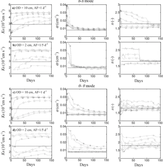
4.2 Parameter identifiability
Figure 7 shows the retrieved parameters Ks, α and n, us-ing both theh-handθ-θ retrieval modes. These graphs de-pict the evolving patterns with the two alternative resolutions (OD=10 cm, AF=1 d−1, and OD=2 cm, AF=1/5 d−1).
The “true” value of αis rapidly identified during the re-trieval process in both modes, but in particular using matric heads. Parameter α is also the least affected by the initial guess of the parameters under scrutiny. Indeed, since param-eter αacts as a scaling factor of the state values in the soil hydraulic property functions, its retrieval is highly sensitive to the convergence rate of the first moment of the state
vec-tor. Vrugt et al. (2001, 2002) found that most of the infor-mation onαis embedded in soil water content observations just beyond the air entry value of the soil. Accordingly, in the present study, the identifiability ofαis probably favoured by the relatively wet states explored in the initial stage of the synthetic experiment.
Figure 5.Ratios of the average RMSE, involving the last 15 days of simulations and the six initial guessed parameter sets, computed between contiguously sampled(a, c)observation depths (OD) and(b, d)assimilation frequencies (AF), with the DSUKF algorithm.
instead, the sensitivity to n was almost three times higher than that of parameterα. This is an interesting aspect, partic-ularly for the issues related to near-surface observations.
Convergence toward the true nis more delayed as com-pared with α. A close inspection of the time series of the retrieved parameters reveals that the convergence of n for the h-based form is mainly driven by the relatively abrupt reductions in soil moisture on about the 50th, 65th, 80th, 100th and 110th days. These gradients generally induce pro-nounced shifts on the updatednvalues for sets S4 and S5, with an initial n=2.6 (see Fig. 7a), while more moderate shifts for sets S1, S3, and S6, which provide systematic un-derestimations ofn. When parameter retrieving does not ac-count for the logarithmic transformation of the matric heads, the sharp decrease in the state variable, taking place on the 110th day, induces in some cases a failure in the retrieval al-gorithm. As shown by Vrugt et al. (2001, 2002), most of the information onnis embedded in observations whose matric heads are located well beyond the inflection point of the soil water retention function.
Using theh-based form of the Richards equation, we gen-erally observe relatively large differences between the evolv-ing patterns stably adoptevolv-ingn <2 orn >2, after the “erratic” first few updates. This behaviour deserves further attention in
future studies. We ascribe these differences to the change in the shape of the soil water capacity, C(h), and of the hy-draulic conductivity,K(h), functions, both linked to the gov-erning equation (Eq. 1), whennchanges fromn <2 ton >2 near saturation, as addressed by Vogel et al. (2001).
Thenvalues retrieved in theθ-θmode exhibit low sensi-tivity to the cited sharp soil moisture gradients. The reduction of the posterior uncertainty in this mode is clearly lower than in theh-h mode for daily assimilations (Fig. 7c), and very small for assimilations every 5 days (Fig. 7d). The conver-gence is more greatly affected by decreasing AF, although the corresponding RMSE values of the retrieved state profiles ap-pear to be rather insensitive to it. The overall performance is affected by the slower convergence of S5. Nevertheless, even for the low-resolution scenario, the method always provides convergent solutions.
Figure 6. Cumulative probability distribution of the RMSE of DSUKF and DEnKF with 50, 35, 25 and 12 ensemble members for both theh-handθ-θmodes.
matric head data simultaneously as part of the statistical in-ference of the soil hydraulic parameters.
One question arising is whether parameterKsis necessar-ily more prone to problems of identifiability than parameters
αandn, given their role in the VGM relationships, or if this is solely a result of the adopted experimental conditions. The limited variability of the observations being assimilated is definitely a factor that can affect a proper identification of
Ks. Several authors highlighted the limitations for a success-ful estimation of VGM parameters, as imposed by the nar-row variability of naturally occurring boundary conditions (Vrugt et al., 2001, 2002, 2003; Scharnagl et al., 2011). A wide range of soil moisture states is required to constrain the soil hydraulic functions reliably. Moreover, the use of a sin-gle metric also conspires against the desired identifiability, as pointed out by Vrugt et al. (2013).
Another possible reason is the fact that the soil water re-tention parameters also feature in the hydraulic conductivity function, thus enhancing the occurrence of high correlations among the model parameters. A strong correlation is found between retrieved parametersnandKs. It is known that this strong interdependence also affects the performance of the VGM model. Especially for certain soil types, Romano and Santini (1999) showed that more successful inverse mod-elling results can be achieved by decoupling the hydraulic conductivity function from the water retention function. As a strategy to reduce the relative uncertainty, Scharnagl et al. (2011) suggested that the parameterKsshould be assessed soon after rainfall events, when soil moisture redistributes more rapidly in the entire soil profile, being essentially driven by gravity.
Table 4 provides further insights into parameter identi-fiability. We illustrate the performance of the adopted ap-proach when the simulations involve only one or two uncer-tain parameters, as compared with the original method con-sidering three uncertain parameters. We compare the average RMSE of the results obtained with the six sets of parameters within the last 15 days, respectively using open loop simula-tions, the state retrieval algorithm SKF, and the DSUKF, both
with OD=10 cm and AF=1 d−1, and with OD=2 cm and AF=1/5 d−1.
Under the conditions adopted for this experiment, the open loop simulations highlight that the uncertainty in the indi-vidual parameters, in particular that ofα andn, has a very different impact on the overall uncertainty, depending on the adopted retrieval mode. The retrieval of matric heads is mainly affected by the uncertainty in parameterα, with an RMSE (1.788) more than five times higher than that with
nandKs. The soil moisture estimations are preponderantly influenced by the uncertainty in parametern, whose RMSE (1.059) is more than three times higher than those computed considering the other two parameters uncertain. In both re-trieval modes,Ksuncertainty has only a limited impact.
When considering two uncertain parameters, the influence of those pairs involving uncertain values ofαin theh-hmode andn in theθ-θ mode is also predominant. In both cases the assumption of uncertainαandnparameters gives rise to the highest RMSE. As can be seen in some cases, the un-certainty of one of these dominant parameters could cause a detrimental effect, similar to that provoked by the combined uncertainty of two or even all three parameters. This result is clear evidence of the marked correlation between them. Again, simple state retrieving always provides poorer results. Careful inspection of the DSUKF behaviour provides fur-ther insights into the non-identifiability ofKs. When we con-sider only the uncertainty ofKs, the method correctly verges to the true value. This can be inferred from the con-siderable reduction of the RMSE when using the DSUKF for daily assimilations (0.035 for the h-h mode and 0.040 for θ-θ ), as compared with the analogous statistics for the open loop solution (0.3 and 0.334, respectively). However, when considering two unknown parameters, we observe (not shown here for the sake of brevity) that of the two pairs in-cluding an unknownKs, the one with the most explanatory parameter (θ for matric heads andnfor soil moisture) still fails to reach the convergence ofKs. For example, when us-ing matric heads and we considerKs andα uncertain, the method still fails to find the correctKs, while when consid-eringKsandnuncertain, all parameter sets tend to converge to the same solution.
We have verified that the states exhibit a cross-covariance withKs two or three orders of magnitude lower than that formed with the other two dominant parameters. Thus, the Kalman gain scarcely affects the prior Ks values consis-tently. We have also verified that both the DEnKF(12) and the DEnKF(50) come across the same problem. However, the DEnKF with 500 ensemble members converges to the true value. Nevertheless, even in this case, minimal deviations of
Figure 7.VGM parametersKs,αandnretrieved with the DSUKF algorithm, using theh-h(a–b)and theθ-θ(c–d)retrieval modes, with
the following assimilation scenarios:(a, c)OD=10 cm and AF=1 d−1;(b, d)OD=2 cm and AF=1/5 d−1. Comparisons account for the six pondered sets of initial parameters: S1(), S2(), S3(∗), S4(1), S5(+)and S6(♦). The dotted line indicates the true value.
Table 4.Average RMSE of the state profiles estimated during the last 15 days of simulations with the six sets of initial parameters (S1– S6), considering either one, two or all three uncertain parameters. The results refer to the open loop simulations, the SKF (involving only state retrieving) with OD=10 cm and AF=1 d−1, the DSUKF with OD=10 cm and AF=1 d−1, and the DSUKF with OD=2 cm and AF=1/5 d−1.
h-hmode θ-θmode
Uncertain Open DSUKF DSUKF Open DSUKF DSUKF
parameters loop SKF OD=10, OD=2, loop SKF OD=10, OD=2, AF=1 d−1 AF=1/5 d−1 AF=1 d−1 AF=1/5 d−1 Ks 0.300 0.174 0.035 0.049 0.334 0.204 0.040 0.070
α 1.788 1.187 0.040 0.065 0.283 0.621 0.058 0.072 n 0.348 0.388 0.038 0.062 1.059 0.345 0.040 0.035 Ks,α 1.777 1.097 0.049 0.081 0.465 0.627 0.071 0.094
Ks,n 0.473 0.514 0.046 0.078 0.888 0.250 0.064 0.093
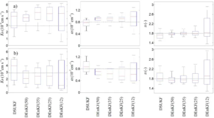
Figure 8. Box plots representing the posterior uncertainty of the parameters by performing DSUKF and DEnKF for 500 randomly chosen sets of initial parameters considering(a)theh-h(b)andθ-θ modes.
within the temporal extent of this experiment), making the model poorly sensitive to the errors of this parameter.
The box plots in Fig. 8 illustrate the posterior uncer-tainty of the parameters estimated with the DSUKF and the DEnKF, considering the 500 randomly chosen sets of initial parameters described in the previous section. The uncertainty ranges of the proposed method are roughly comparable to those obtained by Moradkhani et al. (2005) within the first 150 days of simulation. As emphasized, both methods fail to identify parameterKscorrectly. The decrease in accuracy by assuming only 12 ensemble members, especially during ma-tric head retrieving, is also considerable. Both accuracy and precision of the estimatednvalues are superior using DEnKF under the h-h mode, except for ensembles of 12 members (Fig. 8a). However, for the same scheme, the median of pa-rameterα provided by the DSUKF is less biased than that provided by the nonlinear approach, which overestimates the true value. The performance of the DSUKF is comparable to that of the DEnKF(25), although the interquartile ranges of αandnare slightly smaller with the latter method. The uncertainty regions of the estimated parameters in the h-h
mode are narrower than in theθ-θmode (Fig. 8b). In this lat-ter case, the DEnKF(25) provides wider uncertainty bounds and less accurate estimates of parameters αandnthan the DSUKF.
It could be argued that, given the scope of the present study, a classical calibration method could also provide sim-ilar results. For a more reliable analysis of the pros and cons of the DSUKF, we also implemented gradient iterative algo-rithms based on the Levenberg–Marquardt algorithm (Kool and Parker, 1988), considering the six sets of parameters S1– S6 in the h-h mode. The algorithms were implemented by exploiting the solvers embedded in the Matlab®optimization toolbox.
A major drawback of this technique is its computational time, which is about 30 times larger than that of the DSUKF. About 1 week was needed to generate the a posteriori
distri-bution from the 500 sets of initial parameters. The perfor-mance was also poorer in terms of identifiability. The re-trievednvalues varied between a minimum of 1.64 for S2 and a maximum of 2.23 for S5, while α varied between 0.0055 for S1 and 0.012 cm−1 for S6. Ks remains clearly not identified. The identifiability problems of traditional ap-proaches like this have been documented in the literature (e.g. Kool et al., 1987; Romano and Santini, 1999; van Dam, 2000). Finally, a third difficulty is that these variational meth-ods, although they can be easily implemented, demand some expertise for suitably tuning the parameters involved in the numerical solvers (e.g. tolerance threshold values applied in the numerical algorithm).
4.3 Influence of the type of observed variables with respect to the selected state variables
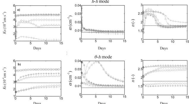
The analyses in the previous section focused on the perfor-mance of theh-handθ-θretrieval modes, i.e. when observed and retrieved variables are of the same type. This allows im-plementing a linear observation equation (Eq. 2), with a stan-dard Kalman filter for state retrievals. Nevertheless, part of the study also focused on the relation between the type of as-similated data and theh-based form orθ-based form of the state equation.
In principle, the numerical algorithm can be structured to assimilate soil moisture observations (or some information linked to it) in theh-based form of the Richards equation by dealing with a nonlinear observation equation, above referred to as theθ-hretrieval mode. This issue can be frequent, given the structure of many widely used simulation models as well as the type of information provided by current remote sens-ing techniques and ground-based sensors.
At this point, it is important to note that the inversion of the observation variable, i.e. converting soil water contents to matric pressure heads by means of a water retention func-tion with guessed (wrong) parameters, would be a serious mistake, because the observations would be significantly bi-ased, incorporating an unpredictable error in the retrieval al-gorithm. By contrast, a nonlinear relationship for transform-ing an exogenous observation variable (such as soil surface temperature from thermal infrared remote sensing) in soil moisture can be directly employed prior to applying the ob-servation operatorHkin Eq. (11).
Figure 9.VGM parametersKs,αandnretrieved with the DSUKF algorithm, using(a)theh-hand(b)θ-hretrieval modes by assimilating
observations every hour, with observation depth OD=10 cm. Comparisons account for the six pondered sets of initial parameters: S1(), S2(), S3(∗), S4(1), S5(+)and S6(♦).
The unscented algorithm is also employed for dealing with the nonlinearity of the observation equation, similarly to what is done for retrieving the parameters. During each time step we propagate the a priori mean and covariance of the matric heads using the SKF, as currently done in theh-hand
θ-θ retrieval modes. When the observation vector becomes available for assimilation, we sample the predicted state vari-able around the mean, following the UKF precepts, using the estimated a priori covariance, P−k. The sample state vectors are propagated through the VGM expression using the a pos-teriori mean of the parameters at timek−1. Then the cross-covariance between predicted states and predicted measure-ments,Pxy,k, and the auto-covariance of these predicted
mea-surements,Pyy,k, are estimated analogously to what is done
for the parameters (Eqs. 20, 22, respectively). The Kalman gain is then estimated asKk=Pxy,k Pυυ,k−
1
, from which the estimations of the a posteriori state mean and covariance are straightforward.
Such linearization clearly incorporates a certain amount of error, which affects the overall identifiability of the unknown parameters. Even the identifiability of parameterαis affected by this assimilation strategy. With low assimilation frequen-cies the algorithm is subjected to persistent failures.
According to such results, while applying the DSUKF, the state variable and observation variable should be preferably of the same type, either in the h-based form or in θ-based form, to avoid the need to linearize the observation equation (Eq. 11) with respect to the states.
Finally, it is useful to see that in an extended Kalman filter framework, the non-zero entries of the linearized observa-tion operatorHk would correspond to the hydraulic
capac-itiesC(h), evaluated in the prior state valuesxˆ−k, at the ob-servation nodes. This provides an idea of the unpredictability of the uncertainty due to the linearization process, as this is strongly influenced by the soil properties.
4.4 Influence of the initial covariance matrices
The DSUKF algorithm, like its analogous approaches, re-quires initial values for the state covariance,P, and the pa-rameter covariance,Pw. The effects of the initial state
covari-ance matrix,P, and of the noise covariance matricesQand Ron the assimilation scheme are clear and have been widely examined (see for example Walker, 1999; Nelson, 2000). The values that should be used for the initial parameter covari-ancePw and the artificial noise covariancesQwandRw, are
less clear and depend on several factors (Nelson, 2000). An initial value 10−2for the diagonal entries ofPw,0 per-formed well for most of the cases, with both soil water con-tents and matric heads as state variables, as found by Nel-son (2000), who also employed normalized parameterization. Once the normalizedPw is fixed, the values of the noise
co-variances depend on the variance of the data, and hence of the state variable.
The effect of evaluating different scenarios accounting for the variability of the parameter noise covariances is illus-trated in Fig. 10, showing the daily retrievals of parameter