Optimisation of a parallel ocean general circulation model
M. I. Beare, D. P. Stevens
School of Mathematics, University of East Anglia, Norwich, NR4 7TJ, UK
Received: 6 January 1997 / Revised: 1 April 1997 / Accepted: 4 April 1997
Abstract. This paper presents the development of a general-purpose parallel ocean circulation model, for use on a wide range of computer platforms, from traditional scalar machines to workstation clusters and massively parallel processors. Parallelism is provided, as a modular option, via high-level message-passing rou-tines, thus hiding the technical intricacies from the user. An initial implementation highlights that the parallel eciency of the model is adversely aected by a number of factors, for which optimisations are discussed and implemented. The resulting ocean code is portable and, in particular, allows science to be achieved on local workstations that could otherwise only be undertaken on state-of-the-art supercomputers.
1 Introduction
As computing technology advances into the age of massively parallel processors (MPPs), ocean models are required that can utilise these state-of-the-art high-performance computers if oceanographers are to con-tinue doing useful research. This is because the study of the ocean and its eect on the climate requires the resolution of features with small spatial scales and long time-scales over large geographic regions. Thus there is a requirement for ever more powerful computers, with large memory. The installation of a national MPP computer in the UK emphasises this technological shift in computing today. The Cray T3D, with 512 processors and a peak performance of nearly 80 G¯op/s is one of the fastest computers in the world. Unfortunately, as one of only a handful of tightly coupled parallel processors of this size, time on the Cray T3D is limited.
It is essential therefore, that processing time is not needlessly wasted for the purpose of developing and testing codes. A parallel platform is required that is cheap and readily accessible, so that parallel codes can be developed and tested before porting to MPPs, such as the Cray T3D. Such platforms are also required for research which, whilst not requiring state-of-the-art supercomputers, still require large computational re-sources.
Recent developments in micro-processor, networking and software technologies have made it possible to treat a cluster of workstations as a single concurrent com-puter. A number of software packages have evolved that allow each connected computer to act as a processor in what is eectively a distributed-memory multi-processor machine, thus providing a platform on which to run parallel code. One popular package in use today is PVM (parallel virtual machine, Geist et al., 1993), which provides the programmer with a simple set of library routines to handle the communication between proces-sors and their synchronisation. Given that many insti-tutions already possess a number of workstations, which are often networked together, and that PVM is a portable public-domain package, the cost of setting up such an environment is just a few man-hours.
Within this paper we will describe the initial imple-mentation of a parallel version of a general-purpose ocean circulation model. When run on a cluster of workstations it is seen that a number of bottlenecks contribute to a poor parallel eciency. Techniques which consider interprocessor communications, load balancing and the model physics are then discussed and implemented to improve the performance of the code. The techniques employed tend to be relatively straight-forward and aim to avoid over-complicating the code with the technical aspects of parallelism. Despite their simplicity, we show that these optimisations give rise to a signi®cant increase in performance, such that the resulting model can be successfully and usefully run in parallel on a cluster of workstations, as well as on massively parallel processors.
Throughout the paper, the workstation cluster used consists of sixteen DEC Alpha AXP 3000/300s, each with 32 Mb of memory. This provides an environment that is homogeneous, although it should be noted that the model may also run in a heterogeneous environment. The cluster is con®gured to provide a general high-performance facility (Beareet al., 1997) and oers a dual networking ring, of Ethernet or FDDI (®bre distributed data interface) for parallel applications.
2 The parallel model
Many of the ocean models run today originate from the three-dimensional ®nite-dierence model, based on the primitive equations of motion, described by Bryan (1969). His pioneering work has withstood the test of time and the only major changes were to optimise the code for running on vector computers and to include additional physics through new parameterisations (Semtner, 1974; Cox, 1984).
More recently the modular ocean model (MOM) code, as described by Pacanowski et al. (1991) and Pacanowski (1995), has been developed as a ¯exible research tool for oceanographers. MOM is modularised, using C-language pre-processor directives, allowing various physical options to be included or excluded as required. The MOM code has also been adapted for array processors, with a reduced set of options, by Webb (1996) and subsequently named MOMA (modular ocean model ± array processor version). Although not strictly a parallel code, MOMA has been arranged in a way that allows the arrays to be vectorised in the vertical and decomposed in the horizontal. With a view to running ®ne-resolution global models on parallel pro-cessors, the rigid lid constraint, as used by Bryan, is removed in MOMA and a free surface is allowed (Killworth et al., 1991). It is the MOMA code upon which the parallel model developed in this paper is based.
The surface of the model ocean is assumed to be split into a two-dimensional horizontal grid. Each grid box is used to de®ne a volume of water that extends from the surface to the ocean ¯oor, organised into a number of vertical (depth) levels. The main prognostic variables required by the model are the baroclinic velocities and tracers (potential temperature and salinity), and the barotropic velocities and associated free-surface height ®eld. The baroclinic variables describe the depth-depen-dent response of the ocean model and the barotropic variables describe the depth-averaged response. All other variables (such as density and vertical velocity) can be diagnosed from the prognostic variables and therefore the dynamic state of the ocean is described. The model variables are discretised using an Arakawa B-grid (Mesinger and Arakawa, 1976), so that the velocities are oset from the free-surface height and tracers. A ®nite-dierence representation of the primi-tive equations is used to predict new values for these variables, thus allowing the model to be stepped forward in time using a series of discrete timesteps. Due to the
fast speed of the external gravity waves, which must be considered when using the free-surface approach, the barotropic and baroclinic components are timestepped separately, with approximately 50±100 barotropic time-steps to each baroclinic timestep.
The model domain used in this paper is that of a pseudo-global ocean extending from 70°S to 70°N. The maximum size of the longitudinal and latitudinal dimensions (Imax and Jmax, respectively) is then
depen-dent upon the required horizontal grid resolution. The vertical extent of the model is de®ned by a number of depth levels, which vary in thickness from about 20 to 500 m. Levels below the ocean ¯oor are masked and thus the topography of the ocean ¯oor is described.
The basic mathematical model contains ®rst- and second-order derivatives, so the ®nite-dierence scheme requires gradients to be determined from values stored in neighbouring grid boxes. Problems occur when stepping forward variables at the perimeter of the model domain, using out-of-bounds array subscripts. The model arrays are therefore over-dimensioned by one grid point in the horizontal extents, creating an addi-tionalouter halo. In the case of a global model the outer halo in the longitudinal direction allows cyclic boundary conditions to be applied, where i1 iImaxÿ1
and iImax i2. In the latitudinal direction
closed boundary conditions are applied to the northern and southern boundaries. The actual domain being modelled is therefore contained within the horizontal extents 2:Imaxÿ1;2:jmaxÿ1.
thus maintaining a modular structure to the code. A general overview of the code, with parallelism as a module option, is as follows:
Start main timestep loop Step tracer values
Step baroclinic velocities
Calculate forcing data for barotropic velocities Start barotropic timestep loop
Step barotropic velocities
Ifparallel version
Send/Receive boundary barotropic velocities
Elsesequential version
Apply cyclic boundary conditions to barotropic velocities
End barotropic timestep loop
Add barotropic velocities to baroclinic velocities
Ifparallel version
Send/Recv boundary baroclinic velocities and tracers
Elsesequential version
Apply cyclic boundary conditions to velocities and tracers
End main timestep loop
The following extract of FORTRAN 77 code high-lights how the C-language pre-processor directives provide parallelism as an option, for the calculation of the baroclinic velocities. The subroutine clinic is called to calculate the new values for the velocity arrays,uand v, at time np for a volume of depth,k, at each i,j grid point. On completion of this process, either the high-level message-passing routines are called, or cyclic boundary conditions are applied, depending on which running mode has been opted for. (It should be noted that it would be more ecient to have the i,j loops inside the subroutine clinic, but the original sequential code did not and so we have left it unaltered, as it has no bearing on the parallel optimisations).
do j = 2, jmax-1 do i = 2, imax-1
call clinic (i, j) end do
end do
#ifdef parallel call send_uv call recv_uv #else
do j = 2, jmax-1 do k = 1, kmax
u (k, 1, j, np) = u (k, imax-1, j, np) u (k, imax, j, np) = u (k, 2, j, np) v (k, 1, j, np) = v (k, imax-1, j, np) v (k, imax, j, np) = v (k, 2, j, np) end do
end do #endif
3 Initial parallel implementation
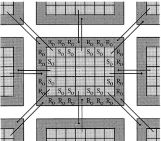
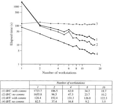
For an initial evaluation of the performance of the code the global model was de®ned with a two-degree horizontal resolution and 32 vertical depth levels. The model grid size is thus 32´ 180´ 69, which leads to a moderate memory requirement of 20 Mb. The model was run for one model day on one to sixteen worksta-tions, with a timestep of 30 min. These runs were repeated over both interconnect systems (Ethernet and FDDI) and the results are plotted, in Fig. 2, alongside a run on a hypothetical, in®nitely fast, interconnect system (achieved by doing no message passing, thus producing incorrect physics, but useful for timing purposes). It should be noted that for any number of Fig. 1. To accommodate the exchange of boundary data, for a
regular two-dimensional decomposition, an additional outer halo,R0, is declared to receive the values that have been calculated and sent from the boundary halo,S0, of adjacent sub domains
Fig. 2. The elapsed time required to model one day of a two-degree global model, with 32 levels, is plotted for runs using 1 to 16 workstations connected via (1) Ethernet, (2) FDDI and (3) a hypothetical, in®nitely fast interconnect. For clarity, the table
workstations the model domain can be decomposed in several ways, and dierent decompositions will often lead to dierent performance times. For example, with six processors the domain can be sub-divided as 6´ 1, 3´2, 2´ 3 or 1´6. So as not to complicate the graph only the best time recorded for a given number of workstations is plotted.
If the model were truly parallel ecient we would expect the performance to increase linearly with the number of workstations, such that two workstations would complete the run in the half the time taken by one workstation, and so on. This is clearly not the case with our model. To begin with the performance of the model does improve, but as more workstations are used the gain in performance decreases. In fact, when the interconnect is Ethernet, the performance becomes worse when more than ®ve workstations are utilised.
The parallel eciency on P processors, PE(P), relative toP0processors, is given by:
PE P ET P0 ET P
P0
P 100;
whereET(P) is the elapsed time onPprocessors. For the FDDI run, assumingP01, we ®nd that PE 16 99%,
which could be conceived as being very good. However, the model shows an initial super-linear speed-up, such that PE 2 368%. This is due to the model being memory bound, when run on a single workstation, leading to a signi®cant overhead when data is paged in and out of virtual memory. By running in parallel on two worksta-tions, the memory requirements of the model are almost halved and (for this model resolution) the memory paging is eliminated. To remove this eect from our calculation of parallel eciency, we chooseP02, which
givesPE(16) = 27%. Considering that lack of memory is often a prominent limitation when running large ocean models, it can therefore, in some cases, be advantageous to run the model on just two or three workstations. It is clear however, that if more workstations are to be used eectively, then the ineciencies associated with the parallelism must be identi®ed and resolved.
Further tests of the model determine three main areas of concern. The ®rst of these is due to the calculation of the free-surface components (the barotropic mode). Compared to the rest of the numerical scheme, the amount of computation required to proceed one time-step is relatively small. However, as explained earlier, the timestep required to solve the free-surface variables must be much smaller than that for the baroclinic velocities or tracers. Hence more timesteps are required in order to step the free-surface forward the same amount of time as a single timestep would for the baroclinic mode. With each of these smaller timesteps there is a need to communicate newly solved values and so a comparatively large amount of time is consumed by communication rather than computation.
The second is due to the positioning of the message passing within the code. Having it coded neatly with the application of cyclic boundary conditions does make it easy to read and understand, but at the same time it is particularly inecient. By exchanging data at the end of
each timestep, after all the calculation has been com-pleted, the processor is left with no alternative but to send its data and then sit idle, waiting for the comple-mentary data to arrive from its neighbours.
The third problem is not so much to do with communications, but due to the regular domain decom-position used. Ocean models are made up of bothocean and land points, but since the model is only concerned with ocean points, the land points are masked and have no computation associated with them. Hence, although the model grid is split into evenly sized sub-domains, these domains do not necessarily consist of an equal number of ocean points and so processors will not always have equal amounts of work. This explains the irregular (saw-tooth-like) speed-up of the ideal case, which is not aected by communication overheads.
Discrepencies in times when running on a single processor are due to the model not checking whether or not it is possible to simply apply cyclic boundary conditions, instead of passing messages to itself. As will be seen later, this check is not essential, since in general, when running on a single workstation, the model will be run in sequential mode.
4 Model optimisations
To improve the parallel eciency of the model code, each of the problem areas highlighted in the previous section will be looked at and the merits of implemented solutions are discussed. It should be remembered that these solutions aim to preserve the code's modularity and scalability, which are desirable features of the model that should not be overlooked in the search for eciency.
4.1 Low computation-communication ratio in the free surface
The free-surface component of the model computes depth-averaged quantities which are stored in a two-dimensional horizontal array of longitudinal and latitu-dinal grid points. Compared to the baroclinic mode there is a reduced number of variables that require solutions and a reduced number of boundary grid points that need to be shared with neighbouring processors. Unfortunately, the number of messages is not reduced and so the latency associated with the message passing is unchanged. Indeed an expensive overhead of PVM, on workstation clusters, is its high latency (Lewis and Cline, 1993) and in comparison to the smaller computation time, the communications become dominant in the time required to compute the free-surface component. The situation worsens as the number of processors increases and sub-domains get smaller.
(with and without message passing). Comparing the two runs in which the message passing is switched o highlights the fact that the barotropic component should compute much faster than the baroclinic part. Yet with message passing switched on, it is immediately clear that the communication associated with the free surface saturates the system, with a devastating aect on the overall performance of the model.
To resolve this problem a technique is adopted to minimise this communication, by trading it for a small amount of extra computation. By introducing further outer halos to the two-dimensional free-surface arrays, a greater amount of information can be exchanged between adjacent processors (as illustrated in Fig. 4). It is then possible to process a number of barotropic timesteps before having to stop and communicate. This approach is similar to that adopted by Sawdey et al. (1995), who de®ne a number of extrafake zones, in order to reduce the frequency of communication.
In the initial implementation processors calculate new values for the dierent variables at each of the grid points within their domain, which is bounded by the haloS0. For each timestep, an exchange of data between
adjacent processors must occur. This message passing involves a processor sending values that have been calculated and stored in S0, out to adjacent processors,
which then receive and store these values in the haloR0.
The processors are then able to proceed with the next timestep.
Consider now the case of adding one extra halo,R1,
to the free-surface arrays, so that two halos can be sent and received for each data exchange. When message passing occurs, data from both the halos,S0 and S1, is
packed and sent to adjacent processors, where it is
received into the corresponding halos, R0 and R1. With
this extra information a processor can calculate new values within the domain bounded byR0(as opposed to
the domain bounded by S0). Hence, on the next
timestep, the values in the R0 halo are already up to
date and so no message passing is required in order to calculate the new values for the domain bounded byS0.
It is at the end of this second timestep that message passing will be required. Thus with one extra halo, message passing need only occur every other timestep and so the overall number of messages that are passed is halved, greatly reducing the relatively expensive latency times. Some extra computation is incurred, however, since values in the halo R0 must be calculated, but this
only need be done on the ®rst of the two timesteps and with computation being so much faster than communi-cation, this overhead is negligible.
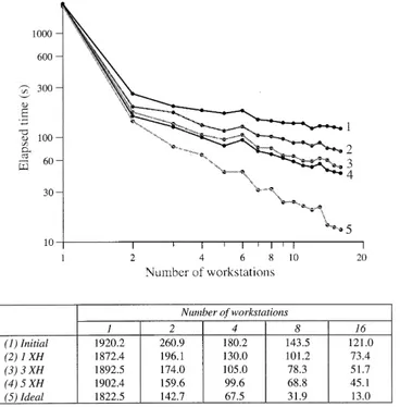
The process of adding extra halos can be generalised to cope with any number of halos and Fig. 5 demon-strates the improved performance that can be achieved as the number of extra halos is increased (so as not to clutter the graph, only odd numbers of extra halos are plotted). The trade-o of communication for computa-tion can give rise to a signi®cantly better performance: almost 300% better for this example when using sixteen workstations connected via FDDI. There is however a limit to how far one can take this method and even with ®ve extra halos the performance gain is beginning to tail o. Increasing the number of extra halos further eventually has a negative eect. Knowing how many extra halos can be usefully employed in this fashion is dependent on the number of workstations being used and the size and resolution of the model domain. One drawback of this optimisation method is however, that the code requires signi®cant modi®cations to the free-surface routine, which add to its complexity.
Fig. 3. Splitting the model into its baroclinic (B/C) and barotropic (B/T) components and running these separately (over FDDI), with and without message passing, highlights the adverse communication overheads associated with the barotropic mode
4.2 Reducing idle processor time
The second ineciency highlighted by the initial imple-mentation is due to the idle time of processors waiting for communications to take place. Having solved all the ®nite-dierence equations for a timestep, the dynamic variables at the boundaries are packed and sent to the appropriate neighbouring processors. Then, with no further calculations possible, the processors have no alternative but to sit idle, waiting for incoming messages to arrive, before they can continue processing. By recording the time spent in the receive routines, it is clear that idle time increases as the number of worksta-tions increases, due to the additional messages travelling on the interconnect.
It is possible to minimise this idle time by rearranging the order in which the domain is parsed. By ®rst calculating just those boundary values that need to be shared, it is possible to send the data and then, whilst this communication is taking place, calculate the values for the remaining inner grid points. If there is sucient work within the inner domain to keep the processor busy, by the time all the new values have been calculated and it is time to receive the data sent from adjacent processors, the messages should have arrived and no idle time will be incurred.
To implement this method, the grid points at the boundary are identi®ed by an ordered list of horizontal (i, j) co-ordinate pairs and stored in an index array, as illustrated by Fig. 6. In detail, the following FORTRAN 77 code illustrates how this is implemented at the top level (again using the routine to predict baroclinic velocities as the example). The index array isouterand the number of outer-halo grid points that it references isnop.
#ifdef parallel do ij = 1, nop
call clinic (outer(1, ij), outer(2, ij)) end do
call send_uv do j = 3, jmax-2 do i = 3, imax-2
call clinic (i, j) end do
end do call recv_uv #else
do j = 2, jmax-1 do i = 2, imax-1
call clinic (i, j) end do
end do
do j = 2, jmax-1 do k = 1, kmax
u (k, 1, j, np) = u (k, imax-1, j, np) u (k, imax, j, np) = u (k, 2, j, np) v (k, 1, j, np) = v (k, imax-1, j, np) v (k, imax, j, np) = v (k, 2, j, np) end do
end do #endif
Figure 7 highlights the potential of this optimisation, with the time taken to complete a model day being more than halved, compared to the initial implementation. This is comparable to the performance increase gained by the previous free-surface optimisation, but is much simpler to implement and leads to a tidier code. A potential disadvantage of this optimisation is that it can lead to an inecient utilisation of cache memory. This is evident when comparing the performance of the parallel codes when run on a single workstation. In the initial implementation the horizontal subscripts (i,j) are parsed in the order in which the arrays are stored in memory, thus making ecient use of the cache. However, by solving the equations for the outer-halo grid points before the inner ones, this eciency is compromised. Despite this, the bene®ts of reducing the idle time of each processor, when running on more than one processor, gives a signi®cant improvement on the overall performance of the model. Also, as suggested earlier, when using a single processor the model will be run in
Fig. 5. Compared to (1) the initial implementation (when using FDDI), the performance of the code is signi®cantly improved as the number of free-surface extra halos (XH) is increased in (2), (3) and (4)
sequential mode and will therefore revert back to the original, more ecient, method of parsing the domain.
4.3 Combining the optimisations
As stated earlier, the technique used to reduce the communication overheads of the free-surface routine complicates the code to some extent and this would be complicated further if, in its general form, it was combined with the technique of overlapping communi-cations with computation. A reduced implementation of the extra free-surface halo technique is therefore opted for. Instead of having a generalised algorithm that is able to cope with any number of extra halos, the number is ®xed to be just one extra halo (i.e. two halos are transferred). This simpli®es the implementation of the optimisation and the code remains comprehensible to the ocean modeller. Furthermore, other ocean physics that may subsequently be added to the code, might also require message passing routines to transfer two halos of data. Such options include the QUICK tracer advection scheme (Farrow and Stevens, 1995) and biharmonic mixing, which have ®nite-dierence representations that span ®ve grid points.
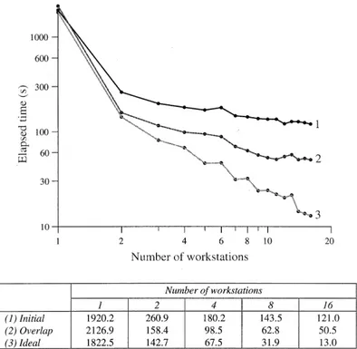
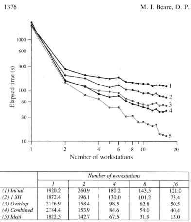
Figure 8 gives a summary of the performance of each of the discussed implementations when run on the workstation cluster connected by FDDI. It is evident that the ®nal optimised code can give rise to a three-times speed-up over the initial parallel implementation, completing one model day in 40.4 s compared to 121.0 s, when using sixteen workstations.
4.4 Load balancing
The use of a regular domain decomposition, which allows for easier parallelisation and greater scalability and modularity, does not however, distribute equal amounts of work to each of the processors. As well as oceanpoints, the model may also consist oflandpoints, which have no computation associated with them. Due to the uneven distribution of these land points within the domain, it is not inconceivable for some processors to end up with more work than others and a few processors may even be allocated no work at all.
To lessen this imbalance, one solution is to divide the domain into a greater number of sub-domains than there are processors (Sawdeyet al., 1995). The objective is to end up with the same number of sub-domains, containing some work, as there are processors. Those sub-domains with no work can then be ignored when allocating sub-domains to processors, as illustrated in Fig. 9.
This approach forms an elegant solution that is easy to implement, requiring changes only to the initial processor allocation phase (which occurs at compilation time, when the machine con®guration is chosen). The advantages are that hopefully no processors will remain idle and that the maximum size of the sub-domains is reduced, thus making the overall performance of the parallel model much better. Also, due to the smaller sized sub-domains, less memory is required per proces-sor. It should be noted that the more processors that are available the more successful this approach will be and it is therefore more suitable when running on MPPs. Table 1 illustrates this technique for the two-degree model with varying decompositions when using 256 processors. For this model an ideal allocation for 256 processors would give a maximum of 1050 ocean points per processor. Although not ideal, this approach can greatly reduce the maximum amount of work per processor and reduce the memory requirements. In this case a 25% reduction is achieved when using a 20´ 15 decomposition.
To get an ideally balanced load would require an irregular two-dimensional decomposition, such as that implemented in the OCCAM (ocean circulation and climate advanced modelling) code and described by Gwilliam (1995). This may however give rise to other problems, not present in our parallel model. In partic-ular, due to the static nature of FORTRAN 77 the arrays must be dimensioned identically for each proces-sor, with scalar variables indicating the true extents of each sub-domain. Thus, if a horizontal decomposition results in a 12 ´6 and a 5 ´14 sub-domain, amongst others, then all arrays would have to be declared as at least 12 ´14. Thus the memory requirements do not necessarily scale well as the number of processors increase, which in turn could inhibit the degree of resolution of the model.
When using just a few processors, it may be bene®cial to restrict decomposition to one dimension and use irregular-sized domains to achieve a more evenly bal-anced load, as used by Sadwey et al. (1995). However, Fig. 7. Reducing idle processor time, by (2) overlapping computation
this approach also suers from memory not scaling with numbers of processors, and care needs to be taken to ensure that memory paging is not reintroduced. When using workstation clusters, it is not necessarily true that all workstations will be of equal power, and another possible solution may be to simply match the sub-domains with higher work loads to the higher-powered workstations.
5 Model evaluation
So far, the results discussed have been for the model running in parallel mode, even for single workstation runs. However, when using a single workstation, it is more ecient to run the model in sequential mode. Firstly, the code does not go through the motions of computing outer-halo values before inner grid values and so cache memory is better utilised. Secondly, the parallel version makes no attempt to identify the fact that it is running on a single workstation and therefore proceeds to do message passing to apply cyclic boun-dary conditions. For a true picture of speed-up it is necessary to compare the performance of the parallel model against that of the sequential one.
In the case of the model that has been used throughout this paper, the sequential version ran for one model day in a time of 1820 s. This implies that the time of 40.4 s when run on sixteen workstations represents a speed-up of 45.0. It has, however, already been stated that memory paging occurs on a single workstation with 32 Mb of memory. To gauge the relative speed-up if this paging were not a factor, the model was run on a 96 Mb workstation. Here the sequential version ran in 259 s, so the estimated scaled speed-up when using sixteen workstations is 6.4. For the code to be more eective over sixteen workstations, it is necessary to increase the size of the model. Running larger, ®ner-resolution ocean models is, however, one of the main rationales for parallelism.
The same pseudo-global model but with a one-degree horizontal resolution was declared and run for one model day, with a 45-min timestep. This time, the 96 Mb workstation was also forced to page memory when running the sequential version and took 2173 s to complete one model day. On the sixteen 32 Mb work-stations, the time taken was just 76 s, representing a speed-up of 28.5. Reducing the number of depth levels to 24 enables the model to ®t into memory on the 96 Mb workstation and a truer picture of speed-up can be seen. With a time of 617 s for the sequential version, a speed-up of 10.9 is achieved by the sixteen workstations, which take 57 s to run. Thus it would take just under 6 h to model 1 year on this cluster.
Increasing the size of the model further, by de®ning a ®ner half-degree horizontal resolution (again with 24 levels), produces a model that just a few years ago, only the largest research groups could envisage running (Semtner and Chervin, 1992) on the fastest supercom-puters of the day. On the cluster, this half-degree global Fig. 8. Compared to (1) the initial implementation and the two
separate optimisations, of (2) one extra free-surface halo and (3) overlapping communications with computation, it can be seen that by (4) combining the optimisations a notable increase in performance is again achieved
Fig. 9a, b. A regular two-dimensional decomposition of an ocean model, containing land (dark-shaded) and ocean (light-shaded) points, can result in some processors having no work (as highlighted inaby processors 1, 13 and 16). By sub-dividing the domain into a greater number of smaller sub-domains, those with no work can be ignored completely and a better utilisation of the sixteen available processors can be achieved (as highlighted inb)
Table 1. 256 processors can be used more eciently by sub-dividing the model into greater than 256 sub-domains and ignoring those domains with no associated work
Processor decomposition
number of sub-domains
max. ocean pts. per sub-domain
sub-domains with some work
16´16 256 1920 223
18´17 306 1600 256
model, with a 22.5-min timestep, takes just under 63 h to complete a 1-year run.
Throughout these tests on the workstation cluster, a one-dimensional decomposition always proved more ecient than a two-dimensional decomposition. This, despite the fact that in general a one-dimensional decomposition actually requires more grid points to be communicated for a given number of processors. The reason for the one-dimensional decomposition being more ecient, as seen before, is due to message latency, not the amount of data being transferred. With a two-dimensional decomposition processors can have up to eight neighbours that they need to communicate with, hence up to eight messages need to be created and sent each time any communication is required. With a one-dimensional decomposition, there is a maximum of only two neighbours and so less messages need be sent.
When ported to the Cray-T3D, with its fast point-to-point interconnect, it was found that interprocessor communications were not as much of a bottleneck as on the workstations. A two-dimensional decomposition was therefore no less ecient than a one-dimensional one: in fact it oers better load-balancing prospects. The bene®ts of the load-balancing optimisation technique described in Sect. 4.4 can be seen when the preceding half-degree model is run on 256 processors. A 16´16 decomposition results in a time of 69.8 s for a 1-day model run, with 33 processors remaining idle, whereas when using a 20 ´15 decomposition the available processors are better utilised and the run takes only 60.6 s to complete. Hence a year-long run can be completed in just over 6 h.
By maintaining the modularity of the code and providing parallelism as a high-level option, the model is not dissimilar in appearance to the original sequential code. It is therefore considered that this will provide ocean modellers with a familiar code that they can use easily, without having to concern themselves with the technical aspects of parallelism. Modifying and extend-ing the code is relatively straightforward, with the addition and development of new physical options being implemented as usual in sequential mode. Once these have been proven correct, the high-level message passing routines can be called from the appropriate points (i.e. wherever cyclic boundary conditions are applied) and the parallel results can then be validated against the sequential results.
Although PVM aids portability, it is not the most ecient of message-passing systems and it is envisaged that at a later date the high-level routines could be rewritten for other portable environments, such as MPI (message passing interface forum, 1994), or include machine speci®c options, such as SHMEM on the Cray T3D.
With the code discussed in this paper it is possible to modify, test and run the ocean model on local worksta-tions, before porting to national MPPs, on which resources are limited. Hence these resources can be used much more productively. Furthermore, groups without access to MPP systems are now able to run large models
on readily accessible local workstations, which may be underutilised overnight.
Acknowledgements. We would like to acknowledge the work of David Webb at Southampton Oceanography Centre towards MOMA, upon which this parallel model has been based. We also wish to thank the Computing Centre at the University of East Anglia for their committment to providing a central service high performance parallel facility, based around their Alpha Farm. M. I. Beare was partially supported by NERC research grants GR3/8526 and GST/02/1012.
Topical Editor D. J. Webb thanks M. Ashworth and S. Maskell for their help in evaluating this paper.
References
Beare, M. I., A. P. Boswell, and K. L. Woods,Managing a central service cluster computing environment,AXIS: UCISA J. Acad. Comput. Inf. Syst., (in press), 1997.
Bryan, K.,A numerical method for the study of the circulation of the world ocean,J. Comput. Phys.,4,347±376, 1969.
Cox, M. D., A primitive equation, three-dimensional model of the ocean, GFDL Ocean Tech. Rep. 1, Geophysical Fluid Dy-namics Laboratory/NOAA, Princeton Univ., Princeton, NJ, 1984.
Farrow, D. E., and D. P. Stevens,A new tracer advection scheme for Bryan and Cox type ocean global circulation models, J. Phys. Oceanogr.,25,1731±1741, 1995.
Geist, A., A. Beguelin, J. Dongarra, R. Manchek, and V. Sunderam,
PVM 3 users guide and reference manual, Oak Ridge National Laboratory, Oak Ridge, Tennessee, 1993.
Gwilliam, C. S.,The OCCAM global ocean model, in Proc. Sixth ECMWF Worksh. on the use of Parallel Processing in Mete-orology, Eds. G. Homan and N. Kreitz, World Scienti®c, London, pp. 446±454, 1995.
Killworth, P. D., D. Stainforth, D. J. Webb, and S. M. Paterson, The development of a free-surface Bryan-Cox-Semtner ocean model,J. Phys. Oceanogr.,21,1333±1348, 1991.
Lewis, M., and R. E. Cline Jr.,PVM communication performance in a switched FDDI heterogeneous distributed computing environ-ment, Sandia National Labs, Tech. Rep., 1993.
Mesinger, F., and A. Arakawa, Numerical methods used in atmo-spheric models, GARP publications series, No.17, World Meteorological Organisation, Geneva, 1976.
Message Passing Interface Forum, MPI: A message passing interface standard, Univ. of Tennessee, Rep. CS-94-230, 1994. Pacanowski, R. C., MOM2 documentation, user's guide and
reference manual, GFDL Ocean Tech. Rep. 2, Geophysical Fluid Dynamics Laboratory/NOAA, Princeton Univ., Prince-ton, NJ, 1995.
Pacanowski, R. C., K. Dixon, and A. Rosati,The GFDL modular ocean model users guide: version 1.0, GFDL Ocean Tech. Rep. 2, Geophysical Fluid Dynamics Laboratory/NOAA, Princeton Univ., Princeton, NJ, 1991.
Sawdey, A., M. O'Keefe, R. Bleck, and R. W. Numrich,The design, implementation and performance of a parallel ocean circulation model, Proc. Sixth ECMWF Worksh. on the use of Parallel Processing in Meteorology, Eds. G. Homan and N. Kreitz, World Scienti®c, London, pp. 523±548, 1995.
Semtner, A. J., A general circulation model for the world ocean, Tech. Rep. 9, Dept. of Meteorology, Univ. of California, Los Angeles, 1974.
Semtner, A. J., and R. M. Chervin,Ocean general circulation from a global eddy-resolving model,J. Geophys. Res.,97,5493±5550, 1992.
Webb, D. J.,An ocean model code for array processor Computers,