Modeling coral calcification accounting for the impacts of coral bleaching and ocean acidification

(1)

BGD

11, 187–249, 2014

Modeling coral calcification

C. Evenhuis et al.

Title Page

Abstract Introduction

Conclusions References

Tables Figures

◭ ◮

Back Close

Full Screen / Esc

Printer-friendly Version Interactive Discussion

Discussion

P

a

per

|

D

iscussion

P

a

per

|

Discussion

P

a

per

|

Discuss

ion

P

a

per

|

Biogeosciences Discuss., 11, 187–249, 2014 www.biogeosciences-discuss.net/11/187/2014/ doi:10.5194/bgd-11-187-2014

Open Access

Biogeosciences

Discussions

This discussion paper is/has been under review for the journal Biogeosciences (BG). Please refer to the corresponding final paper in BG if available.

Modeling coral calcification accounting

for the impacts of coral bleaching and

ocean acidification

C. Evenhuis1,2, A. Lenton1, N. E. Cantin3, and J. M. Lough3

1

Centre for Australian Weather and Climate research, CSIRO, Marine and Atmospheric Research, Hobart, Tasmania, Australia

2

Now at the Plant Functional Biology and Climate Change Cluster, Faculty of Science, University of Technology, Sydney, NSW, Australia

3

Australian Institute of Marine Science, PMB 3 Townsville MC, Townsville, QLD 4810, Australia

Received: 13 December 2013 – Accepted: 13 December 2013 – Published: 6 January 2014

Correspondence to: A. Lenton (andrew.lenton@csiro.au)

(2)

BGD

11, 187–249, 2014

C. Evenhuis et al.

Title Page

Tables Figures

◭ ◮

Back Close

Full Screen / Esc

Discussion

P

a

per

|

D

iscussion

P

a

per

|

Discussion

P

a

per

|

Discuss

ion

P

a

per

|

Abstract

Coral reefs are diverse ecosystems threatened by rising CO2 levels that are driving

the observed increases in sea surface temperature and ocean acidification. Here we present a new unified model that links changes in temperature and carbonate chem-istry to coral health. Changes in coral health and population are able to explicitly

mod-5

elled by linking the rates of growth, recovery and calcification to the rates of bleaching and temperature stress induced mortality. The model is underpinned by four key prin-ciples: the Arrhenius equation, thermal specialisation, resource allocation trade-offs, and adaption to local environments. These general relationships allow this model to be constructed from a range of experimental and observational data. The different

char-10

acteristics of this model are also assessed against independent data to show that the model captures the observed response of corals. We also provide new insights into the factors that determine calcification rates and provide a framework based on well-known biological principles for understanding the observed global distribution of calcification rates. Our results suggest that, despite the implicit complexity of the coral reef

environ-15

ment, a simple model based on temperature, carbonate chemistry and different species can reproduce much of the observed response of corals to changes in temperature and ocean acidification.

1 Introduction

Coral reefs are among the most biologically complex ecosystems, supporting a

di-20

verse range of species, and providing critically important ecosystem services such as food, resources for livelihoods and coastal protection. Despite this, they are facing an unprecedented rate of environmental change in response to increasing atmospheric CO2 levels driving observed increasing ocean temperatures and ocean acidification

(Hoegh-Guldberg et al., 2011; Doney et al., 2009).

(3)

BGD

11, 187–249, 2014

C. Evenhuis et al.

Title Page

Tables Figures

◭ ◮

Back Close

Full Screen / Esc

Discussion

P

a

per

|

D

iscussion

P

a

per

|

Discussion

P

a

per

|

Discuss

ion

P

a

per

|

The ocean plays a key role in slowing the rate of climate change by absorbing and sequestering approximately 25–30 % of the annual atmospheric carbon dioxide (CO2) emissions (Le Quéré et al., 2013). As CO2 enters the ocean (slowing the rate

of ocean warming) a number of changes in seawater chemistry occur, collectively re-ferred to as ocean acidification (OA). For Scleractinian corals one of the most significant

5

consequences of OA is the decrease in the concentration of carbonate ions (CO−

3),

which together with calcium are used to construct their skeletons. The primary min-eral phase of calcium carbonate formed by Scleractinian corals is aragonite. Studies have demonstrated that the capacity of corals to calcify is reduced as the saturation state of aragonite (Ωarg) declines in response to rising CO2concentrations in seawater 10

(Schneider and Erez, 2006; Langdon and Atkinson, 2005; Pandolfi et al., 2011). Pro-jections suggest that future rates of coral reef community dissolution may exceed rates of CaCO3production (calcification), leading to net loss of reef framework and coral reef

habitat within this century (Silverman et al., 2009; Hoegh-Guldberg et al., 2007). As atmospheric CO2 and other greenhouse gas concentrations continue to rise, 15

ocean temperatures will continue to increase e.g. in the tropical ocean, where the greatest abundance and diversity of corals are found, a net increase of 0.09◦_C/decade

in the period 1950–2011 has been reported (Lough, 2012). Scleractinian corals are sensitive to increasing ocean temperatures because of the close symbiotic relationship between the coral host and their endosymbiotic dinoflagellate (Symbiodiniumspp.).

Ex-20

perimental studies have shown that calcification is enhanced as temperature increases, up to an optimum value that is typically a few degrees below the seasonal maximum temperature, and beyond this optimum temperature calcification rates rapidly decline (Al-Horani, 2005; Cooper et al., 2008; Cantin et al., 2010). This increase in tempera-ture will ultimately lead to corals ejecting their simbiont dinoflagellates, zooxanthellae,

25

(4)

inten-BGD

11, 187–249, 2014

C. Evenhuis et al.

Title Page

Tables Figures

◭ ◮

Back Close

Full Screen / Esc

Discussion

P

a

per

|

D

iscussion

P

a

per

|

Discussion

P

a

per

|

Discuss

ion

P

a

per

|

sity of global mass bleaching events in recent decades resulting in an estimated loss in hard coral cover of approximately 18 % and a decline in the dominant populations at a rate of 1–2 % per year (Hoegh-Guldberg et al., 2011; Wilkinson, 2008).

Historically, the risk of corals bleaching due to extreme temperatures has been mod-eled by the degree heating week or month metrics e.g. Donner et al. (2005). Because

5

these metrics were built on empirical observations of bleaching they can be viewed as a statistical heuristic. It is therefore difficult to link degrees heating metrics to the changes in biological function that result from stress, or to extend the metrics to include differential species response or to account for thermal adaptation. As a consequence, it is difficult relate how the risk of bleaching given by the DHW metric impacts

calcifi-10

cation rates e.g. Buddemeier et al. (2008). Furthermore, there are a number of ways for estimate the thermal thresholds that underpin the DHW metric, and little consen-sus exists as to which approach is best suited to a given location. Studies have shown that the projected responses of coral reefs in some regions are highly sensitive to way the thermal threshold is calculated (Donner, 2011), and the distribution and severity of

15

coral bleaching throughout individual coral reefs can be extremely patchy (Baird and Marshall, 2002; Berkelmans et al., 2004). Studies investigating the past and future re-sponse of corals usually focus on the impact of increasing ocean temperatures leading to bleaching (Cantin et al., 2010; van Hooidonk et al., 2013; Frieler et al., 2013) or on ocean acidification (Ricke et al., 2013).

20

In this work we acknowledge that coral reefs are very complex ecosystems and any complete model would require describing a vast array of processes ranging from global scale climate systems down to wave action on the local reef scale, and capturing the closely coupled interaction between hundreds of species of plants and animals. At present such a model at the reef scale is both beyond our current theoretical

under-25

(5)

BGD

11, 187–249, 2014

C. Evenhuis et al.

Title Page

Tables Figures

◭ ◮

Back Close

Full Screen / Esc

Discussion

P

a

per

|

D

iscussion

P

a

per

|

Discussion

P

a

per

|

Discuss

ion

P

a

per

|

This “bottom up” approach allows the response of coral ecosystems to climate change to be inferred from changes in the rate at which corals calcify.

In this paper we present a new model that provides a unified description of coral calcification linking bleaching-related mortality, recovery from bleaching, and growth. Our goal is to provide a simple description of these processes that is motivated by the

5

underlying physiological mechanisms and, where possible, validated against experi-mental observations. The model aims to provide a unified approach to modeling coral growth and health that captures the differences between species and across locations. One of the important features of our model is how the two critical thresholds that de-fine the temperature response are determined by assuming that corals have evolved

10

to maximize their growth over the historical period. By taking into account ocean acid-ification and temperature our model is able to better resolve the relative influence of these two stressors.

The paper is structured as follows; the methods section describes the formulation of the model and estimation of parameter values based on a synthesis of existing

15

observational and experimental data. In the results section the new model is assessed against independent data that was not used in the formulation of the model. We show that, despite the implicit complexity of the coral reef environment, a simple model based on temperature, carbonate chemistry and different species can reproduce much of the observed coral response. We also demonstrate how the model provides insights into

20

processes that give rise to the linear relationship between average temperature and calcification rate observed by Lough and Barnes (2008) and Lough (2008). Finally in the discussion we compare this new model to existing models that combine ocean acidification and temperature, discuss the limitations of our model, and identify key areas for future research.

(6)

BGD

11, 187–249, 2014

C. Evenhuis et al.

Title Page

Tables Figures

◭ ◮

Back Close

Full Screen / Esc

Discussion

P

a

per

|

D

iscussion

P

a

per

|

Discussion

P

a

per

|

Discuss

ion

P

a

per

|

2 Methods – model construction

In this section we describe how our new model of calcification rate is constructed (Eq. 1). This model aims to capture the general, transferable relationships between growth, bleaching and calcification based on experiments and observations of corals from different locations and from different from taxa. The calcification rate (G) is given

5

in Eq. (1).

˙

G

Calcification rate

= gC

Calcifcation constant

Irradiance

Qday

Temperature dependence

z }| {

α(T,Topt,∆T)

Adapted response

β(Topt,Ea)

Thermal envelope

Aragonite dependence

z }| {

γ(Ω;Ωcp,κ) Csp

Species constant

PH

Population of healthy coral

(1)

The calcification rate is depends on the level of light (Qday), the sea surface temperature (α,β), the aragonite saturation state (γ), whether the species is fast or slow growing (Csp), and on the population of healthy corals (PH). The effect of light is accounted for 10

by using the expression for the daily average solar irradiation that depends only the day of the year and latitude.

One of the novel aspects of this model is the inclusions of the way in which corals respond to temperature. The commonalities in the temperature response between species have been extensively investigated using the Metabolic Theory of Ecology

15

(Dell et al., 2011; Brown et al., 2004) andDynamic Energy Budget(Nisbet et al., 2000) frameworks. In the case of corals, the temperature dependence is more complicated as normal physiological performance relies on the symbiotic relationship between the coral polyp and the algal dinoflagellate, Symbiodinium. This complication is reflected in the sophistication of coral models that model host and symbiont responses (Muller

20

(7)

BGD

11, 187–249, 2014

C. Evenhuis et al.

Title Page

Tables Figures

◭ ◮

Back Close

Full Screen / Esc

Discussion

P

a

per

|

D

iscussion

P

a

per

|

Discussion

P

a

per

|

Discuss

ion

P

a

per

|

bleaching, recovery and calcification depend on temperature and differ systematically between species.

We will now explain each of the terms in Eq. (1), first quantifying the response of corals to aragonite saturation state γ, after which the form of the adapted tempera-ture responseα is established. This allows the equations that describe changes in the

5

population and health of individual corals (includingPHandCsp) to be determined.

Sub-sequently, by linking the population changes to the local temperature regime a general method for finding the adapted range (Topt,∆T) is developed. Finally, by relating the

rates of calcification between different reefs, the form of the thermal envelope is set (β).

10

2.1 Aragonite dependence (γ)

Coral reefs are primarily composed of aragonite, the metastable form of calcium car-bonate produced by hermatypic corals. Calcification rates are commonly related to the aragonite saturation state (Ωarg), which is a measure of the inorganic solution

equilib-rium between solid aragonite and calcium and carbonate ions in solution. The

depen-15

dence of the calcification rate with the seawater carbon system has been extensively investigated (Erez et al., 2011; Pandolfi et al., 2011; Schneider and Erez, 2006; Putron et al., 2010) but remains poorly understood. Experiments have shown that corals trans-port seawater to the site of calcification within the basal calicoblastic ectoderm and are able to manipulate its carbonate chemistry, thereby up-regulating the aragonite

sat-20

uration state in favour of CaCO₃ precipitation (Al-Horani, 2005). The precipitation of aragonite at the site of calcification may be inorganic, biologically mediated or some combination thereof (Allemand et al., 2011). Given these complexities, our model em-ploys an empirical relationship to describe how calcification depends on the aragonite saturation state of seawater.

25

(8)

satura-BGD

11, 187–249, 2014

C. Evenhuis et al.

Title Page

Tables Figures

◭ ◮

Back Close

Full Screen / Esc

Discussion

P

a

per

|

D

iscussion

P

a

per

|

Discussion

P

a

per

|

Discuss

ion

P

a

per

|

tion state for 18 experiments, from which two broad classes of response are evident (an example of a more comprehensive list of experiments can be found in Table 2 of (Erez et al., 2011)). In the first class (drawn in blue), calcification declines linearly with aragonite saturation, ceasing aroundΩ≈1. While in the second class (drawn in red), the response is more plateaued. The response is comparably more flat aroundΩ =3.5

5

and a steep fall off when Ω<1. The reason for the two responses is not yet under-stood (for a recent review see Chan and Connolly, 2013). Current hypotheses include differences in experimental techniques, differences between tropical and temperature corals, and whether the corals were given sufficient time to adapt to the change in sea-water chemistry. However, the available experimental evidence suggests that the linear

10

response is most likely related to nutrient concentrations (Pandolfi et al., 2011). The observed linear and plateaued responses are fitted to a modified version of the Michaelis–Menten curve. This curve is widely used to describe biochemical reactions that are enzyme mediated. Initially this curve increases linearly, after which it saturates and approaches an asymptotic value. The following function (Eq. 2) is used to fit the

15

dependence of calcification on Aragonite saturation state:

γ(Ω;Ωc,κ) Aragonite dependence=

Modified Michaelis–Menten

z }| {

Ω−1+0.1κ 1+κ(Ω−1+0.1κ)

Cross-over point

z }| {

1+κ(Ωc−1+0.1κ)

Ωc−1+0.1κ

Normalisation

z }| {

1

3.5₋1 . (2)

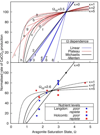
This functional form is controlled by two parameters;κ determines the curvature, and Ωcsets the point at which curves with different values ofκ intersect. The upper panel

of Fig. 1 plots the 18 experimental calcification rates, normalised so that atΩ =3.5 the

20

calcification rate is 100 %. This normalisation means that the cross-over point for both responses is also Ωc=3.5. If κ=0 2.1 simplifies to (Ω−1)3.51₋1, which is the linear

response that starts atΩ =1 and is normalised to 100 % atΩ =3.5. In Fig. 1 it can be seen how increasingκincreases the curvature of the response, and how the 0.1κterm shifts the point at which the curve goes to zero. This effect is most apparent forκ=5

(9)

BGD

11, 187–249, 2014

C. Evenhuis et al.

Title Page

Tables Figures

◭ ◮

Back Close

Full Screen / Esc

Discussion

P

a

per

|

D

iscussion

P

a

per

|

Discussion

P

a

per

|

Discuss

ion

P

a

per

|

for which calcification ceases atΩ =0.5. By fitting theγto the plateaued experimental results we determined that a typical value for the curvature isκ=2.

In the lower panel of Fig. 1 the results of Langdon and Atkinson (2005) and Holcomb et al. (2012) are used to determine the cross-over point. These experiments measured calcification rates under both nutrient poor and replete conditions. A linear response

5

was observed in nutrient poor conditions, whilst a plateaued response was observed in replete conditions. The results are normalised so that the (linear) responses is 100 % when Ω =3.5. By fitting the curve for γ with κ=2 to the nutrient replete results the crossover point was determined to beΩcp=2.6.

In the upper panel of Fig. 1 there is a considerable spread in the results. Most of

10

these experiments measure net calcification rate, which includes negative effects from processes such as dissolution. Although it is difficult to estimate the magnitude of the dissolution rate, it is expected to be larger for in situ measurements than for laboratory experiments, given the processes that control dissolution e.g. Andersson and Gledhill (2013).

15

By comparing with experimental measurements of calcification rates it was possi-ble to reduce the aragonite responseγ to one of two possibilities, a linear (κ=0) and plateaued (κ=2 andΩcp=2.6) response (Fig. 1). Unless indicated otherwise, the

lin-ear calcification response is used, however a plateaued response could be substituted as desired.

20

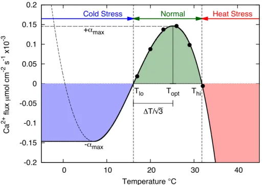
2.2 Modelling the temperature and population responses (α,β,Csp,PH)

The temperature response (in Eq. 1) is comprised of both the adapted response (α) and thermal envelope (β). The adapted response captures how corals respond to temper-ature fluctuations on timescales of hours to weeks, and dictates the tempertemper-ature range over which symbiosis occurs. The adapted response can be considered as the fast

25

(10)

BGD

11, 187–249, 2014

C. Evenhuis et al.

Title Page

Tables Figures

◭ ◮

Back Close

Full Screen / Esc

Discussion

P

a

per

|

D

iscussion

P

a

per

|

Discussion

P

a

per

|

Discuss

ion

P

a

per

|

Broadly speaking, experimental observations of coral can be viewed as probing ei-ther the adapted response or the ei-thermal envelope. Laboratory experiments that ma-nipulate temperature and measure the change in coral’s biological functions explore the adapted response. While studies that compare the historical rates of coral calcifi-cation from localcifi-cations with different climates can be used to infer the thermal response.

5

Separating these responses by their time scales allows us to quantify key information about the response of individual coral species (C_sp) and the health of the population to changes to temperature (PH).

2.2.1 The adapted temperature response (α)

The adapted response describes how symbiosis in coral is affected by temperature

10

fluctuations on daily to monthly timescales. Although the shape of the adapted re-sponse is general, specifics such as the adapted low (Tlo) and high temperatures (Thi)

depend on reef location. The shape of the adapted response is based on experimental observations of a range of processes, including photosynthesis (Jones et al., 1998), calcification (Al-Horani, 2005; Jokiel and Coles, 1977), growth (Edmunds, 2005),

re-15

production (Jokiel and Guinther, 1978) and respiration (Edmunds, 2008). All of these traits exhibit a common behaviour; the rate reaches a maximum at an optimum temper-ature and steeply decreases to zero on either side to define the adapted tempertemper-ature range. The similarities in the response across a range of biological processes in corals suggests that these processes most likely respond in unison to the breakdown of

sym-20

biosis which we model with the adapted response function,α.

Mathematically, α (in Eq. 1) is constructed as a piecewise smooth combination of a cubic polynomial and a constant as shown in Eq. (3):

α(T;Topt,∆T)=

   

  

T > T_lo:

Cubic Polynomial

−c(T−Tlo)

(T−Tlo) 2

−∆T2

Normalisation

4

∆T4−δ

T < Tlo:−αmax Constant

(3)

(11)

BGD

11, 187–249, 2014

C. Evenhuis et al.

Title Page

Tables Figures

◭ ◮

Back Close

Full Screen / Esc

Discussion

P

a

per

|

D

iscussion

P

a

per

|

Discussion

P

a

per

|

Discuss

ion

P

a

per

|

where:

Tlo=Topt−

1 √

3∆T

Thi=Tlo+ ∆T

The maximum of this function is atTopt, and is positive betweenThiandTlo. This function 5

depends on only the adapted range, which can be expressed as (Tlo,Thi) or (Topt,∆T).

When the temperature is in this range corals grow, calcify, reproduce and recover from bleaching, whilst outside of this range, bleaching and mortality occur. Consistent with observations the magnitude of the slope atThiis twice that atTloe.g. Al-Horani (2005).

Figure 2 shows the fit of the adapted range (α) functional form to the experimental

10

measurements of Al-Horani (2005). The normalisation term (Eq. 3) plays a central role by rewarding thermal specialisation. The rationale behind this term and its effect are discussed fully in Sect. 2.2.7. Although other researchers have modelled temperature response of corals with cubic polynomials, we found that the additional constraints imposed on the form of α aid in the interpretation and comparison of experimental

15

results.

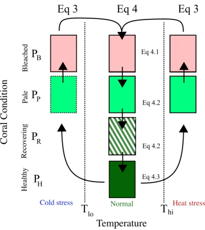
2.2.2 Modelling changes in population (PH)

A core part of this model is its ability to describe changes in the health and population of corals. The model uses coral cover as a state variable, which is further classified into four states: healthy, recovering, stressed, and bleached. The four states come

20

from reports of coral condition from the literature (e.g. Reef Base: www.reefbase.org). The states can be viewed as a qualitative measure of the health of the symbiosis, capturing more quantitative measures such as density of the zooxanthellae or levels of lipid stores.

The four states and the transitions between them are shown schematically in Fig. 3

25

(12)

BGD

11, 187–249, 2014

C. Evenhuis et al.

Title Page

Tables Figures

◭ ◮

Back Close

Full Screen / Esc

Discussion

P

a

per

|

D

iscussion

P

a

per

|

Discussion

P

a

per

|

Discuss

ion

P

a

per

|

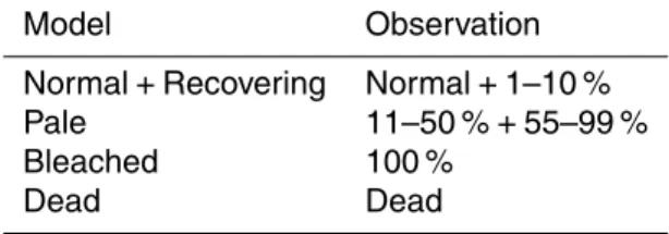
– Healthy corals grow and calcify at normal rates. When stressed, healthy corals turn pale.

– Pale corals have ejected some or all of the their zooxanthellae, and growth calcifi-cation are impaired. When stress is prolonged, pale corals will further bleach, but under normal temperatures pale corals transition to recovering phase of rebuilding

5

tissue reserves.

– Bleached corals have lost the majority of their zooxanthellae, do not grow or repro-duce, and face the risk of mortality. Under normal temperatures bleached corals transition to pale, while further stress leads to mortality.

– Recovering corals are those that have only recently reacquired zooxanthellae

af-10

ter bleaching, and although healthy in appearance, do not reproduce or calcify at the same level as healthy corals. When stressed, recovering corals turn pale, otherwise they return to healthy under normal conditions.

The transition between the states is modelled by a system of 1st order differential equa-tions. The rate of these transitions is modulated by a common temperature response,

15

(13)

BGD

11, 187–249, 2014

C. Evenhuis et al.

Title Page

Tables Figures

◭ ◮

Back Close

Full Screen / Esc

Discussion

P

a

per

|

D

iscussion

P

a

per

|

Discussion

P

a

per

|

Discuss

ion

P

a

per

|

2.2.3 Bleaching

The transition of coral from healthy ( ˙PH) to pale ( ˙PP), to bleached ( ˙PB), and finally to

dead is given by the following first order differential equation:



  

˙

PH

˙

PR

˙

PP

˙

PB



 

=_BleachinggB

constant

Csp

Species constant

Insolation

Qday

z }| {

α(T,Topt,∆T) Adapted response

β(Topt,Ea) Thermal envelope



  

+1 0−1 0 0 0 0 0 0 0 1₂ −12

0 0 0 +14



  



  

PH

PR

PP

PB



 

 (4)

5

Where the constantgBdetermines the time scale of the bleaching which is applicable

for all locations and species,C_spis the species constant, andαandβare the transient and steady state temperature response curves, respectively. Importantly, the rate of bleaching is proportional to the species constant (Csp). For example, faster growing

corals will bleach faster and have higher mortality, while slower growing corals will be

10

more resistant to bleaching, consistent with observations. This differential response to temperature or (Csp) can be understood in an energy budget framework as a

trade-off between growth and heat tolerance. There is a wide range of mechanisms and strategies that corals can use to mitigate the damage from bleaching. For example, corals that store more lipids or have more tissue biomass are able to better survive

15

bleaching (Anthony et al., 2009), the coral and the symbiont may employ anti-oxidants to deal with the increase in reactive oxygen production or express heat shock proteins to deal with the increased temperature (Baird et al., 2009), or corals may increase feeding rates to meet the short fall in autotrophic energy (Houlbreque and Ferrier-Pages, 2009). However, any strategies that a coral employs to defend against heat

20

stress, energy deficiencies impact on the energy budget and reduce the allocation of resources to growth and reproduction (Rodrigues and Grottoli, 2006; Michalek-Wagner and Willis, 2001).

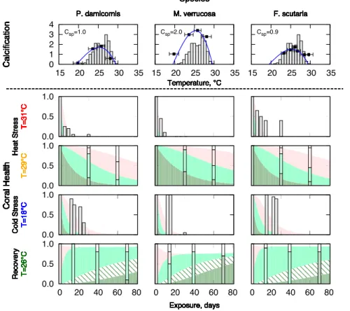
The transitions between the four coral states, shown schematically in Fig. 3, corre-spond to the entries in the 4×4 matrix in Eq. (4). The first row of Fig. 4 shows the fit

(14)

BGD

11, 187–249, 2014

C. Evenhuis et al.

Title Page

Tables Figures

◭ ◮

Back Close

Full Screen / Esc

Discussion

P

a

per

|

D

iscussion

P

a

per

|

Discussion

P

a

per

|

Discuss

ion

P

a

per

|

of the adapted response curve to the measurements of calcium carbonate calcification rate from Jokiel and Coles (1977). This allowed the adapted temperature range (Tlo,Thi)

and the species constant (Csp) to be determined for each coral species. As thermal

re-sponse in these short-term experiments plays no role we ignore this rere-sponse and set the thermal envelope toβ≈1. The species parameter was defined to be 1.0 forP.

dam-5

icorniscorals. As adapted range is the same for the three corals,Toptthe rates of the

transition (healthy to pale, pale to bleached, bleached to dead) can be determined by fitting the model to the experimental observations forP. damicornis. The agreement be-tween the resulting patterns from the model output and the experimental observations is very good (Fig. 4), and the bleaching constant is calculated to beg_B=8.d−1_{. This}

10

allowed the species constants forM. verrucosa(Csp=2) andF. scutaria (Csp=0.9) to

be calculated.

2.2.4 Recovery from bleaching

After exposure to elevated temperatures, corals undergo a range of recovery processes (Fig. 3). Following bleaching the coral host acquires significantly less autotrophic

car-15

bon based energy from the depleted symbiont community within in its tissue (see re-view by Glynn, 1996). As recovery processes continue following thermal stress, the coral host metabolizes tissue reserves and relies on heterotrophic feeding to compen-sate for energy limitations (Thornhill et al., 2011). Rate of recovery processes which include, repopulation of the symbiont community, tissue repair and replenishing

ener-20

getic tissue reserves will depend upon the severity of the thermal stress and the colony condition prior to the thermal stress event. Collectively these recovery processes are modelled using the following set of 1st order differential equations (Eq. 5), which dif-fer from Eq. (3) with the addition of an additional recovering state ( ˙PR). This describes

corals which are in the recovering state and, despite having a healthy appearance,

dis-25

(15)

re-BGD

11, 187–249, 2014

C. Evenhuis et al.

Title Page Abstract Introduction Conclusions References Tables Figures ◭ ◮ ◭ ◮ Back Close

Full Screen / Esc

Printer-friendly Version Interactive Discussion Discussion P a per | D iscussion P a per | Discussion P a per | Discuss ion P a per |

ported in the experimental results of Jokiel and Coles (1977).

    ˙ PH ˙ PR ˙ PP ˙ PB   

=_MortalitygM

constant Csp Species constant Insolation Qday    

0 0 0 0 0 0 0 0 0 0 0 0 0 0 0−1

        PH PR PP PB     (5)

+ gR

Recovery constant Csp Species constant Insolation Qday Temperature dependence

z }| {

β(Topt,Ea) Thermal envelope



  

0+12Csp 0 0

0−1₂Csp+Csp 0

0 0 −Csp+8/Csp

0 0 0 −8/Csp

        PH P_R PP PB    

Again, the form of the equations was determined by fitting to the results of Jokiel and

5

Coles (1977), the values of the continued mortality and recovery time constants were determined as gM=0.04d−

1

and gR=0.2d− 1

. The first term in Eq. (5) represents the continued risk of mortality that bleached corals face even when the temperature falls back into the adapted range, and reflects the limited ability of corals to survive without zooxanthellae. This term is also proportional to the species constant Csp, as 10

slower growing corals have larger lipid stores that enable them to survive longer with-out zooxanthellae. The second term in Eq. (5) represents the recovery from bleaching as the corals return from bleached to pale, pale to recovering, and finally to healthy. The bleached to pale transition term differs from the other terms, as it is inversely propor-tional to the species constant. This means that, in general, faster growing corals react

15

more negatively to bleaching (more rapid bleaching, increased risk of mortality when bleached and slower to re-establish symbiosis), the exception being that the transition from pale to healthy is more rapid in faster than in slower growing corals. At present, without additional data on recovery dynamics it is difficult to determine whether this is an artefact resulting from over fitting the uncertainties in the experimental data or

20

(16)

BGD

11, 187–249, 2014

C. Evenhuis et al.

Title Page

Tables Figures

◭ ◮

Back Close

Full Screen / Esc

Discussion

P

a

per

|

D

iscussion

P

a

per

|

Discussion

P

a

per

|

Discuss

ion

P

a

per

|

Figure 3 shows the comparison between the model output using Eqs. (4.1) and (4.2). Noting that the modelling results show the recovering state ( ˙PR), which was not

re-ported in the experimental results of Jokiel and Coles (1977).

2.2.5 Growth constant (GC)

The coral growth term in the model has the highest uncertainty as it represents the

5

combined effect of many processes. This term (Eq. 6) encompasses the growth of individual corals, natural mortality, recolonisation of dead coral structures, reproduction and constraints on growth from the maximum habitat size are all described by a single equation for growth in our model. The equation used for the growth term in the model is given in Eq. (6).

10



  

˙

PH

˙

PR

˙

PP

˙

P_B



 

=_BleachinggC

constant

Csp

Species constant

Insolation

Qday

z }| {

β(Topt,Ea)

Thermal envelope

(6)

·

Logistic bottleneck

z }| {

K−

X

P_i



  

+1 0 0 0 0 0 0 0 0 0 0 0 0 0 0 0



  



  

PH

PR

PP

PB



  

The term (K−PPi) is referred to as thelogistic growthin ecological modelling serves to reduce the growth rate as the total population (PPi) as it approaches the carrying

15

capacity (K) of the location. In this workK =1 (i.e. 100 % carrying capacity), however there is scope to model external stressors that could reduce the carrying capacity of a location, such as storm damage or sea-level rise, by allowingK to vary temporally.

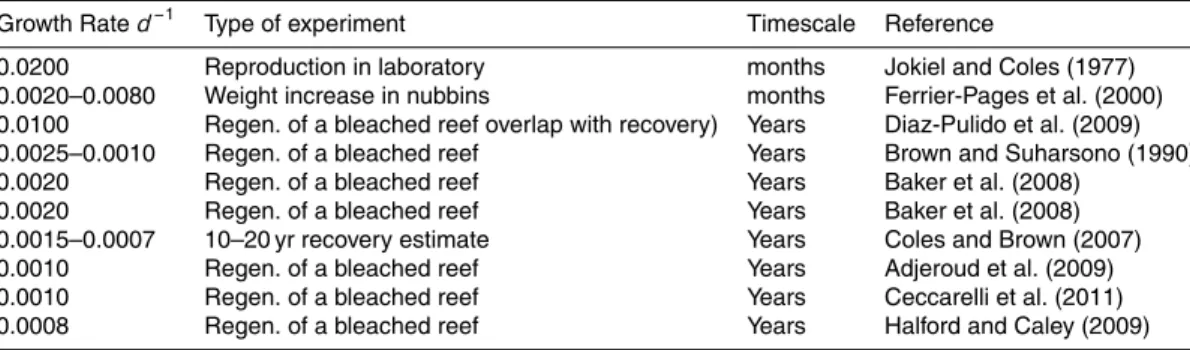
The range of values for the growth constants is large (Table 2) as there are many contributing factors to this term such as whether the measurements are taken in

labo-20

(17)

BGD

11, 187–249, 2014

C. Evenhuis et al.

Title Page

Tables Figures

◭ ◮

Back Close

Full Screen / Esc

Discussion

P

a

per

|

D

iscussion

P

a

per

|

Discussion

P

a

per

|

Discuss

ion

P

a

per

|

very hard to get a firm estimate of this parameter, we selected the value of the growth constant (gC) to be 0.002d−

1

, based on a synthesis of in situ published that report the return of coral coverage after a disturbance such as bleaching.

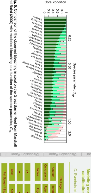
2.2.6 Species response (Csp)

Studies have identified the role of species as a confounding variable when

compar-5

ing observations of corals. In the previous section differences between species were captured in the model by the species constant Csp that modulates the relative rates

of key processes. As discussed previously, corals that grow and calcify faster and are more sensitive to bleaching are modelled as havingCsp>1, whilst corals that calcify

and grow slower but are more resistant to bleaching are modelled as havingCsp<1. 10

Therefore it is useful to an estimate of the expected range of the species constant. In the previous sections the species constant was determined from direct measurements of the calcification rate, which in turn was used to infer the relative rates of growth, bleaching and recovery.

In this section an estimate of the species constants of a wide range of coral species

15

is derived from observations of the large-scale bleaching that occurred in 1998 on GBR (Marshall and Baird, 2000). These allow the species of coral to be linked to the species constantCsp and can serve as a guide when setting up the model for a specific coral

reef. Figure 6 compares the bleaching observations to the model output for a range of the species constants. The adapted temperature range ofTlo=20.0 andThi=30.6 20

used in the model was estimated from historical temperatures from the Hadley SST (Rayner et al., 2003) product and from reported bleaching events from ReefBase (www. reefbase.org). The model was run from 1 January 1998 to 12 March 1998 using in situ recorded temperature for Pelorus Reef (available from the Australian Institute of Marine Science website). It can be seen that the value of the species constant varied

25

(18)

BGD

11, 187–249, 2014

C. Evenhuis et al.

Title Page

Tables Figures

◭ ◮

Back Close

Full Screen / Esc

Discussion

P

a

per

|

D

iscussion

P

a

per

|

Discussion

P

a

per

|

Discuss

ion

P

a

per

|

This maybe explained by differences in how pale and bleached corals were classified in this study from the classification of Jokiel and Coles (1977) that was used to construct this model.

The differences in bleaching response between species may also, in part, be due to differences in the depths at which the species lived, as shown for Montastrea

an-5

nularis(Baker and Weber, 1975). By way of illustration, consider two corals that have an identical bleaching response (T_lo,T_hi, andC_sp); one is found in shallow water whilst the other is found only in deeper water. The shallower coral will be exposed to a larger range of temperatures and higher light intensities, therefore, will bleach to a greater degree than the deeper coral. Field based observations also indicate that bleaching is

10

generally most severe on reef flat and upper reef slope habitats, to a depth of_∼4–6 m (Oliver and Berkelmans, 1999). As we do not explicitly include depth in the model it appears that the deeper corals will be more tolerant to bleaching, i.e. thatCspis lower

for coral species that are typically found in deeper habitats.

2.2.7 Determining the adapted temperature range (α)

15

It has been widely observed that coral bleaching thresholds are only a few degrees above and below the extremes of the local temperatures, which implies that corals are facing a high risk of bleaching as temperatures change (Hoegh-Guldberg, 1999). From this observation two conclusions are drawn that are central to the model. Firstly, corals are able to adapt to their local environment by changing their adapted response

20

(α). And secondly, corals must derive some benefit from having their thermal thresh-old close to temperature extremes that offsets the increased risk of bleaching. This motivates the inclusion of a reward for thermal specialisation within the model.

α(T;Topt,∆T)=

   

  

T > Tlo:

Cubic Polynomial

−c(T−Tlo)

(T−Tlo) 2

−∆T2

Normalisation

4

∆T4−δ

(7)

(19)

BGD

11, 187–249, 2014

C. Evenhuis et al.

Title Page

Tables Figures

◭ ◮

Back Close

Full Screen / Esc

Discussion

P

a

per

|

D

iscussion

P

a

per

|

Discussion

P

a

per

|

Discuss

ion

P

a

per

|

where:

Tlo=Topt−

1 √

3∆T

Thi=Tlo+ ∆T

Based on the wide diversity within the Symbiodinium genus (Baker, 2003; Jones, 2008),

5

corals have the potential to specialise through symbiosis. This can be considered as a resource allocation issue; i.e. the changes a coral undergoes to adapt to a wide tem-perature range, be it biochemical or physiological, will come at some cost to the coral. The normalisation term in Eq. (7) describes this thermal specialisation, through either rewarding or penalising coral calcification rates. In the model large adapted

tempera-10

ture range results in reduced rates of growth and calcification, which is consistent with the hypothesis of (Oliver and Palumbi, 2011) and (Castillo et al., 2012).

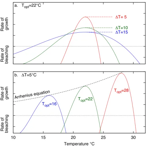
The simplest way to reward thermal specialisation is to conserve the area under the adapted response curve (i.e. to normalise the functionα over the temperatureTlo

to Thi). If the area under α is conserved then the maximum of α is proportional to 15

∆T−1_{. If identical corals from two sites are compared and the second site has twice}

the temperature range of the first, the model would predict that the rates of growth and calcification at the second site would be half that of the first site. This is a common choice for normalisation of reaction norms, for example see Gilchrist (1995). The effect of thermal specialisation is illustrated in Fig. 7 which shows how calcification rates are

20

reduced as the adapted range increases.

Having established how thermal specialisation is rewarded, the procedure for finding the adapted range of corals is now outlined (Tlo,Thi). By assuming that the corals have

adapted to their local climate the adapted temperature range can found by maximis-ing the calcification rate over an historical period. Strictly speakmaximis-ing calcification is not

25

(20)

BGD

11, 187–249, 2014

C. Evenhuis et al.

Title Page

Tables Figures

◭ ◮

Back Close

Full Screen / Esc

Discussion

P

a

per

|

D

iscussion

P

a

per

|

Discussion

P

a

per

|

Discuss

ion

P

a

per

|

equation), which leaves calcification as the best available variable to serve as a proxy for Darwinian fitness.

Maximising the total calcification rate finds the best trade-offbetween the competing effects of bleaching (which favours a large adapted range) and thermal specialisation (which favours a small adapted range). Figure 7 gives an illustration of this trade-off

5

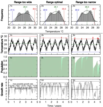
between population and productivity by showing the relative contribution of coral pop-ulation and calcification rate when the adapted temperature is too wide, is just right, or is too narrow. The first column shows how when the adapted range is too large the histogram of the temperatures falls entirely under the transient temperature curve. Al-though no bleaching occurs so the population is the greatest of the three, its possible

10

calcification rate is the lowest due to the penalty imposed by the large adapted range. The third column show when the adapted range is too small a significant fraction of the histogram of temperatures falls aboveThi. Although the maximum possible rate of

calci-fication is higher than the optimal or wide specialisation scenarios, the high frequency and intensity of bleaching reduces the healthy population that in turn reduces the net

15

calcification.

The optimal temperature range strikes the balance between the risk of bleaching and net calcification rate, resulting in the highest realised growth rate of the three potential thermal specialisation scenarios (Fig. 6). Some bleaching will occur, however thermal tolerance has been optimized to maximise the balance between potential total

calcifi-20

cation and bleaching frequency. This fits nicely with the observations and understand-ing of bleachunderstand-ing in corals. The widely made observation that corals are 1–2◦_{C from}

bleaching would appear to be a fragile choice for organism. However, in the framework of our model this seeming risk choice makes sense; corals have adapted to their local temperature regime to maximise both their productivity and population.

25

Therefore, by maximising the total calcification rate the adapted range (Tlo and Thi)

(21)

BGD

11, 187–249, 2014

C. Evenhuis et al.

Title Page

Tables Figures

◭ ◮

Back Close

Full Screen / Esc

Discussion

P

a

per

|

D

iscussion

P

a

per

|

Discussion

P

a

per

|

Discuss

ion

P

a

per

|

records or to climate model output. This leaves the species constantCsp as the sole

remaining “free parameter” in the model.

2.3 The thermal envelope (β)

The final term to be determined in our model is the thermal envelope, which is used to relate differences in productivity of corals between different locations. In the previous

5

sections the absolute rate of calcification was not important as it was used only to determine the adapted temperature response. In this section an absolute value is put on the rate of calcification.

Determining a value for the rate of calcification is challenging, as there is a wide vari-ation in measured calcificvari-ation rates between different experimental protocols. Kleypas

10

and Langdon (2006) identified seven experimental approaches for measuring calcifica-tion rate, with spatial scales ranging from individual corals to whole reef communities, and temporal scales from hours to millennia. Here we have used the large dataset of calcification rates forPoritescompiled by Lough et al. (Lough and Barnes, 1997, 2000; Poulsen et al., 2006; Lough, 2008). This dataset allows the calcification rate of a single

15

species (Porites) to be compared across 60 unique geographic locations (Shi et al., 2012; Scoffin et al., 1992; Poulsen et al., 2006; Lough, 2008; Fabricius et al., 2011; Edinger et al., 2000; Cooper et al., 2012).

The thermal envelope is characterised by examining how the rate of calcification varies between locations due to differences in the local temperatures. The increase

20

in biological function with average temperature is a well-known phenomenon and is commonly modelled using the Boltzmann–Arrhenius curve. This Arrhenius equation can be viewed as an upper bound on the thermal efficiency of corals. The details of how this energy is used by a specific coral is determined by the adapted response

α and the species constantCsp. To this point we have ignored the contribution to the 25

(22)

BGD

11, 187–249, 2014

C. Evenhuis et al.

Title Page

Tables Figures

◭ ◮

Back Close

Full Screen / Esc

Discussion

P

a

per

|

D

iscussion

P

a

per

|

Discussion

P

a

per

|

Discuss

ion

P

a

per

|

other locations. This is achieved by defining the thermal envelope as:

β(Topt,Ea)=exp



 

Ea

R 1

300− 1

T_opt





, (8)

where E_a is the activation energy and R is the gas constant. Figure 7b shows the effect of changing the average temperature Topt whilst the temperature range ∆T is

held constant.

5

However, problems arise if the thermal envelope is used with the adapted response from Eq. (7). From Eq. (7) it can be seen that growth rate a given temperature is pro-portional to ∆T−1_{. By being inversely proportional to the adapted range the adapted}

response curve decreases too slowly when the temperature range is large and in-creases too quickly when the temperature range small. The problem of slow decrease

10

when the temperature large is large can be illustrated by considering how the thermal envelope and the adapted response curve behave as the upper threshold increases while keeping the lower threshold fixed. For the temperatures of interest the Arrhenius term can be approximated as an exponential, and by expressingToptin terms ofTloand

∆T, the increase from the thermal envelope is can be approximated as:

15

β(Topt,Ea)≈exp



 

Ea

RTopt−300

3002



 ∝exp

_E

a

R3002

∆T

√ 3

. (9)

The problem is that the exponential increase in the thermal envelope outpaces the decrease from the normalisation term∆T−1_{. Consequently, as the upper threshold is}

increased at some point the increase in thermal envelope is bigger than the penalty incurred for having a large adapted range. This means that when the calcification rate

20

is maximised it is possible forThi to increase without bound. One way to address the

(23)

BGD

11, 187–249, 2014

C. Evenhuis et al.

Title Page

Tables Figures

◭ ◮

Back Close

Full Screen / Esc

Discussion

P

a

per

|

D

iscussion

P

a

per

|

Discussion

P

a

per

|

Discuss

ion

P

a

per

|

the extended Boltzmann Arrhenius equation (Dell et al., 2011). Alternately, limiting the size of the adapted range or increasing the penalty for having a large adapted range could also address the problem.

A similar problem arises when the temperature range is small. As the area under the adapted response curve is conserved the maximum rate (the rate atTopt) is pro-5

portional to∆T−1_{, which results in clearly unrealistically behaviour when the adapted}

temperature range is small. As a thought experiment consider a coral that has adapted to three locations that have the same average temperature and temperature range of 10◦_{C, 1}◦_{C and 0.1}◦_{C. If the adapted temperature curve is normalised the model}

would predict the 1◦_{C and 0.1}◦_{C sites to have the 10 and 100 times the growth rate of}

10

the 10◦_{C site. One would expect some increase in growth rate to occur as the range}

shrinks as a result of thermal specialisation, but for it to ultimately approach some limit. A solution would be to place limits on the minimum temperature range or to “roll-off” the normalisation factor to a constant as the temperature range decreases.

The most direct solution to the above two problems is to replace the normalisation

15

term by an exponential. The exponential replacement is designed to decay faster than the thermal envelope and to match the behaviour of the normalisation term around 10◦_{C. The updated version of the adapted response curve is now:}

α(T;Topt,∆T)=

   

  

T > Tlo:

Cubic Polynomial

−(T−Tlo)

(T−Tlo) 2

−∆T2

Normalisation

4_×10−4_exp[

−0.33(∆T−10)]

(10)

20

where:

Tlo=Topt−

1 √

3∆T

(24)

BGD

11, 187–249, 2014

C. Evenhuis et al.

Title Page

Tables Figures

◭ ◮

Back Close

Full Screen / Esc

Discussion

P

a

per

|

D

iscussion

P

a

per

|

Discussion

P

a

per

|

Discuss

ion

P

a

per

|

Using the equation above the exponential normalisation factor can outpace the rise in the thermal envelope for activation energies up to 500 kJ mol−1_{, which is well above the}

range of biochemical reactions.

Having established a mechanism to avoid the spurious high temperature runaway the calcification constant in Eq. (1), the normalisation correctionδfrom Eq. (7) and the

ac-5

tivation energyEain Eq. (8) are found by fitting the model to the observed calcification

rates. For each location the adapted temperature range was determined by maximising the calcification rate over the historical period (1900–1970). The relative distribution of aragonite saturation state was estimated from GLODAP (Key et al., 2004) and WOA (Conkright et al., 2002). Given that the changes in calcification due to changes in ocean

10

acidification are small over the historical period, a single (time invariant) value of arag-onite was used in each location.

The average calcification rate over the historical period was calculated by min-imising the residual between the calculated and observed calcification rates, shown in Fig. 8. From this the rates for the values of gC=0.038 g cm−

2

d−1_, _δ₌_{0.33 and}

15

E_a=50 kJ mol−1_{were determined. Interestingly, the magnitude of the calcification}

con-stant puts calcification processes on the same timescale as growth and reproduction. Similarly, the activation energy falls within the range that is observed for biological pro-cesses (Dell et al., 2011). The valueδ >0 reflects the inefficiency in the allocation of resources to small temperature ranges.

20

In the final section of the results a simplified version of the model is constructed that is used to show the linear relationship between calcification rate and average temper-ature observed by Lough and Barnes can emerge from the Arrenhius relationship, the penalty imposed on large adapated ranges, and from the correlation between average temperatures and temperature ranges.

(25)

BGD

11, 187–249, 2014

C. Evenhuis et al.

Title Page

Tables Figures

◭ ◮

Back Close

Full Screen / Esc

Discussion

P

a

per

|

D

iscussion

P

a

per

|

Discussion

P

a

per

|

Discuss

ion

P

a

per

|

3 Results and assessment

Having outlined the construction of the model in the previous section, here the model is assessed against three sets of experimental results that were not used in the construc-tion of the model. The model was constructed starting with the smallest spatial and temporal scales (minutes, organism) and systematically built up to the largest

(cen-5

turies, geographic). As no one single experiment is able to bridge these spatial and temporal timescales, we validate the model with a set of experiments that tests a sub-set of the components. In this way, although in isolation a single experiment assesses only part of the model, when taken in aggregate they demonstrate the overall perfor-mance and robustness of the model.

10

In the final section of the results a simplified version of the model is constructed that is used to show the linear relationship between calcification rate and average temper-ature observed by Lough and Barnes can emerge from the Arrenhius relationship, the penalty imposed on large adapted ranges, and from the correlation between average temperatures and temperature ranges.

15

3.1 Aragonite, adapted response, local temperature range

The first assessment of our model compares the simulated calcification rates with those reported by Erez et al. (2011) (Fig. 11; originally reported in Schneider and Erez, 2006). In this experiment calcification of the coralAcropora eurystomawas measured as a function of aragonite saturation state and temperature. The comparison between

20

the experimental results and the model output is shown in Fig. 9 this assesses the ex-pression used for calcification (Eq. 1) and links adapted temperature response to the local climate.

The experimental data in the left hand panel of Fig. 9 clearly displays the linear re-sponse to aragonite saturation. In order to achieve good fit with the linear rere-sponse

25

(26)

BGD

11, 187–249, 2014

C. Evenhuis et al.

Title Page

Tables Figures

◭ ◮

Back Close

Full Screen / Esc

Discussion

P

a

per

|

D

iscussion

P

a

per

|

Discussion

P

a

per

|

Discuss

ion

P

a

per

|

gross calcification rates from the reported values. The calcification rates were mea-sured at three temperatures and show that optimal calcification rates were achieved at 24◦_{C. The model highlights the strong dependence of calcification on temperature, as}

calcification rates across a range ofΩarg are reduced at temperatures above (29◦C)

and below (21◦_{C) the optimal temperature (}

∼25◦C).

5

The right hand panel of Fig. 9 demonstrates how the maximum observed calcification rates are linked to the local or adapted temperature range. The temperatures thresh-olds that define the adapted response curve were found by optimizing the calcification rate, as described in Sect. 2.2.7, and is plotted over the histogram of the historical SSTs as shown in Fig. 9. Maximum calcification is observed at 25◦_{C, 3}◦_{C below the}

10

local seasonal maximum SST, and 5◦_{C above the local seasonal minimum SST. The}

dashed lines connecting the left and right panels of Fig. 9 shows the dependence of calcification rate on both the aragonite saturation state and temperature and empha-sizes that temperature is the dominant driving enhancing calcification across a range ofΩarg.

15

3.2 Population changes, species, optimizing to local climate

The second assessment of our model utilises the observations of the 1998 bleach-ing event on the GBR reported by (Baird and Marshall, 2002). Specifically, this work reported how four different species of coral bleached and recovered over subsequent months. The translations of the states used to classify the condition of the coral from

20

the observations to the 5 states used in the model are given Table 3.

The model was initialised with 100 % healthy coral, and in situ temperatures used for 1998 (available from the AIMS website: www.aims.gov.au). Figure 10 shows good agreement between the observations and model and provides a test of the ability of the model to reproduce the observed response. The values for the species constants

25

(27)

BGD

11, 187–249, 2014

C. Evenhuis et al.

Title Page

Tables Figures

◭ ◮

Back Close

Full Screen / Esc

Discussion

P

a

per

|

D

iscussion

P

a

per

|

Discussion

P

a

per

|

Discuss

ion

P

a

per

|

The third assessment of the model uses the reciprocal transplant experiment of How-ells et al. (2013) which highlights the importance of the adapted range. This experiment monitored the health of corals that were exchanged between reefs on the central and southern GBR. Corals relocated from the southern to the central site experienced tem-peratures above their adapted range and bleached due to heat stress, whilst corals

5

transferred from the central to the southern site experienced temperatures below their adapted range and bleached due to cold stress.

The two locations, Nelly Bay (central GBR) and Miall Island (southern GBR), have significantly different climatologies, which is reflected in their respective adapted ranges.

10

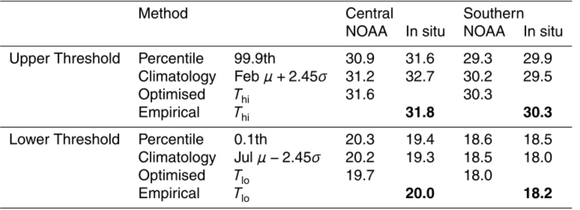
Table 4 shows the thermal thresholds for the two locations, calculated by four meth-ods using two SST time series (the NOAA AVHRR product and in situ temperature logger records). The first approach estimates the adapted range by calculating ex-treme percentiles of the SST distribution – in this case the percentiles correspond to 1-in-3 year temperature extremes. The second adapts a common bleaching metric

15

(Maximum Monthly Mean plus variance). The third employs the optimisation procedure outlined in section 0 that maximises the calcification rate over the historical period. Fi-nally, in the empirical approach the upper and lower thresholds were manually adjusted to reproduce the experimental observations. The spread in values highlights some of the difficulties in estimating thermal thresholds which impact on the severity and timing

20

of coral bleaching and recovery.

There are a number of challenges when a coral’s adapted range is calculated from an SST product and then compared to bleaching observations.Firstly, the low spatial resolution (0.25◦ _{for NOAA (Reynolds et al., 2007), 1}◦ _{for HADISST, Rayner et al.,}

2003) means that temperature fluctuations at the scale of the reef are averaged out,

25