E
NERGY AND
E
NVIRONMENT
Volume 2, Issue 2, 2011 pp.267-276
Journal homepage: www.IJEE.IEEFoundation.org
Microgrids: Energy management by loss minimization
technique
A. K. Basu
1, S.
Chowdhury
2, S.P. Chowdhury
21
Electrical Engineering Dept., Jadavpur University & 20/2, Khanpur Road, Kolkata 700047, India.
2
Electrical Engineering Department, University of Cape Town & Private Bag X3, Menzies Building, Room-517, Rondebosch, Cape Town 7701, India.
Abstract
Energy management is a techno-economic issue, which dictates, in the context of microgrids, how optimal investment in technology front could bring optimal power quality and reliability (PQR) of supply to the consumers. Investment in distributed energy resources (DERs), with their connection to the utility grid at optimal locations and with optimal sizes, saves energy in the form of line loss reduction. Line loss reduction is the indirect benefit to the microgrid owner who may recover it as an incentive from utility. The present paper focuses on planning of optimal siting and sizing of DERs based on minimization of line loss. Optimal siting is done, here, on the loss sensitivity index (LSI) method and optimal sizing by differential evolution (DE) algorithms, which is, again, compared with particle swarm optimization (PSO) technique. Studies are conducted on 6-bus and 14-bus radial networks under islanded mode of operation with electric demand profile. Islanding helps planning of DER capacity of microgrid, which is self-sufficient to cater its own consumers without utility’s support.
Copyright © 2011 International Energy and Environment Foundation - All rights reserved.
Keywords: Differential evolution algorithms, Particle swarm optimization, Loss sensitivity index,
Microgrid
.1. Introduction
between network and generation planning. But in U.S. regulation, there is a provision for utility to connect DG at strategic locations on the grid. Now incentives are given to DNOs to interconnect DGs of modest penetration for reduction of losses. [1-3]
Cost is an important attribute in microgrid planning which involves identification of best DERs along with its siting, manner of interconnection to the utility and schedule of deployment. Energy management system (EMS) make best use of DERs to attain at highest economic as well as technical efficiency by analyzing various cost saving opportunities of microgrid, like line loss of network, which account for 5% to as much as 20% of generation. These losses display a U-shaped trajectory depending on the siting and sizing of DERs in the network. If DERs are placed and sized strategically a significant reduction of loss could be obtained. Injection of DER power at lower voltages tends to reduce losses but where these greatly exceed demand, overall losses may increase. Like consumers demand, loss is, also, a demand by the network itself on the utility and extra generation is required to provide by utility to meet this demand and it involves extra cost. Microgrid owner must be paid incentive by utility as its reduction of line loss benefit helps utility to avoid provision of extra generation. [1, 2, 4, 5]
Many researchers had worked on siting and sizing of distributed energy resources (DER) based on network loss minimization. Griffin et. al.[6] used loss sensitivity technique along with power system simulation for engineering (PSS/E) software package; Greatbanks et.al. [7] used both voltage and loss sensitivity indices along with reactive power compensation and capacitor bank sizing algorithm; Nara et.al. [8] used tabu search (TS) method; Abdelaziz et.al.[9] used simple genetic algorithm (GA) and evolutionary approach (EA); TS is faster and better convergence characteristic compared to simulated annealing method [8]. When simple GA [9] is compared with EA, EA is found better at all average values of losses. Heuristic and arithmetic crossover operation and two point mutation in EA is superior to any other method. Carpinelli et. al. [10] used Monte Carlo simulated based Raleigh correlated random variables, genetic algorithm (GA) and decision theory for siting and sizing of uncertain wind generator with an object of minimization of total cost of network structure, which include construction, residual, management costs and cost of losses.
The present paper conducts two separate studies for energy management decision of siting and sizing of DERs in 6-bus and 14-bus radial micro-grids. Locations of DERs are determined by loss sensitivity indices (LSI) and optimal sizes are determined using differential evolution (DE) technique with minimization of line losses in microgrid. DE is found to yield better and faster solution, satisfying all the constraints, both for uni-modal as well as multi-modal systems, using its different crossover strategies [11, 12]. It is a simple population-based stochastic parallel search evolutionary algorithm for global optimization. To compare the DE results, PSO has been used. PSO technique is conceptually simple, easy to implement, robust to control parameters and computationally efficient [13].Optimal losses and corresponding sizing of DERs are determined at various demands of load profile under islanded modes of operations.
The contents of this paper are organized into following sections. Section 1 on introduction is followed by section 2, which provides detailed formulations of the problem. Section 3 gives a brief overview of DE technique. Section 4 details the DE algorithms in the context of present problem. Section 5 includes necessary figures, results and discussions of two study cases. The conclusion is drawn in section 6. References are appended last.
2. Problem formulations
Present paper has two parts –(1) optimal siting of DERs in the microgrid network and (2) optimal sizing of them. First part is handled using loss sensitivity indices and for second part DE optimization technique is used.
2.1 Optimal siting of DERs
Optimal siting of DERs are determined on the basis of loss sensitivity indices and its equation (1) is based on Newton-Raphson load flow method [16].
[ ]
⎥⎦ ⎤ ⎢ ⎣ ⎡ ∂
Ρ ∂ =
Ρ ∂
Ρ ∂
i l L
i l
J
δ
*
1 (1)
2.2 Optimal sizing of DERs [15]
∑
∑
= =
+
=
=
ni i n
i i
Loss
P
P
V
P
MinP
2 1
1
)
|,
(|
δ
(2)Subject to PQR Constraints:
• Bus voltage tolerance limit
max min i i i
U
U
U
≤
≤
• Limit on the active and reactive power generation of the DER
min max
i i i
P
≤
P
≤
P
min max
i i i
Q ≤Q ≤Q
• Line flow limits (e.g. must be below thermal limits) and takes care of internal congestion of the micro-grid
max
ij j
S
≤
Si
• Limit on active and reactive power injection to slack bus:
P1 and Q1 are respectively active and reactive power injection to the slack bus. Under this constraint, the
capacity of DERs obtained by simulation will be the installed capacity of micro-grid, without reserve, to meet the peak demand under islanding i.e. grid outage.
; 0
1 ≅
P Q1 ≅0
where
P
i is the active power injection at i-th bus, n is total number of buses, P1 (slack bus powerinjection) is dependent on other bus voltage magnitudes |V| and angles δ.
3. Overview of differential evolution technique
Differential Evolution (DE) is an extremely powerful optimization algorithm from evolutionary computation due to its excellent convergence characteristics and a few control parameters. DE uses a population IP of a generation ‘g’of size ‘NP’, composed of floating point-encoded individuals (Eq.3) that evolve to reach an optimal solution. Each individual Xig, is a vector (Eq. 4) that contains as many
parameters as the problem decision variables D, called ‘genes’. The population size ‘NP’ is an algorithm control parameter selected by the user, which remains constant throughout the optimization process.
IPg = Xig, i= 1, . . ., NP (3)
Xig = xi,jg , j= 1, . . .,D (4)
3.1 Initialisation
The optimization process in DE is carried out with three basic operations: Mutation, crossover and selection. The first step of this algorithm is to create an initial population of ‘NP’ vectors, by randomly generating individuals within the boundary constraints (Eq. 5):
IP0 = xij0 = randi,j * (Hj − Lj) + Lj (5)
where ‘rand’ function generates values uniformly in the interval [0,1]. The fitness function is evaluated for each individual. Hj and Lj are upper and lower limit of boundary constraint of jth population.
For each generation the individuals of the population are updated by means of a ‘Reproduction’ scheme. Therefore, for each individual ‘ind’ a set of other individuals ' '
π
is randomly extracted.3.2 Mutation / differentiation
The mutation operator is in charge of introducing new parameters into the population. A set of randomly extracted individuals
π
={
ξ ξ
1, 2,...,ξ
n}
is necessary for ‘Differentiation’. To achieve this mutantoperator creates mutant vectors by perturbing a randomly selected vector (
ε
) with a difference vector δ. the result of ‘Differentiation’, so called ‘trial’ individual, is*
F
ω ε
= +
δ
(6)2 1
δ ξ ξ
=
−
andε ξ
=
3. The scaling constant, F, is an algorithm control parameter used to control theperturbation size in the mutation operator and improve algorithm convergence. ξ1, ξ2 and.ξ3 are randomly
chosen vectors and are selected anew for each parent vector.
3.3 Crossover/ recombination
After, the trial individual ‘ω’ is recombined with updated one ‘ind’. ‘Recombination’ represents a typical case of a ‘genes’ exchange. The trial one inherits genes with some probability. Thus,
{
if randj < Cr otherwise jj
ind
ω
ω
=
(7)
where j = 1, . . . ,D and Cr ∈[0, 1) is the ‘constant of recombination’. Crossover constant Cr is an
algorithm parameter that controls the diversity of the population and aids the algorithm to escape from local optima.
3.4 Selection
‘Selection’ is realized by comparing the cost function values of updated and trial individuals. If the trial individual has lower value of the cost function, then it replaces the updated one.
{
( )
(
)
if f
f ind
ind
ind otherwise
ω
ω
≤
=
(8)It may be noticed that there are only three control parameters in this algorithm. These are ‘NP’(population size), ‘F’ (constants of differentiation) and ‘Cr’(constants of recombination). As for the termination conditions, one can either fix the number of generations ‘gmax’ or a desirable precision of a
solution. DE offers several variants or strategies for optimization. These can be denoted by DE/x/y/z, where x refers to the vector used to generate mutant vectors, y the number difference vectors used in the mutation process and z the crossover scheme used in the crossover operation.
4. DE based algorithmsforloss minimization
The proposed algorithm is implemented with MATLAB 6.5 language on a Pentium-IV PC. Gauss-Siedel load flow method has been embedded into DE algorithms for finding out the optimal solution. Let pi =
[(Pi1, Pi2,…..PiN)] be the trial vector designating ith particle of the population and i=1,2,3…..n. The
elements of pi are real power outputs of N generating units. The objective is to minimize function as
mentioned in (Eq. 2). The computational steps in respect to case of 6-bus radial system are as follows, 14-Bus case is similar:
•
Read the input data:- Bus data, Line data , no. of buses (n), no. of lines (nl) and all other data under section 5.•
Initialize the particles of the population in a random manner according to the limits of each unit including individual dimensions, search points and velocities. These initial particles must be feasible candidate solutions that satisfy the PQR operating constraints, as mentioned in section 2.2.•
Fitness function, Min(PLoss) is evaluated as per equation (Eq. 2) for each individual set of thepopulation.
•
Apply the Differentiation (Mutation) operation on the population as per Eq.6.•
Apply the Crossover (Recombination) operation on the population, generated after mutation operation of Step 4, as per Eq. 7.•
The population settings after Step 4 & 5, which perform better against the fitness function, are selected to be part of the next population according to (Eq. 8).•
If current iteration is greater than or equal to the maximum iteration, keep the result in an Array and stop; otherwise repeat the Steps 3 to 6.•
Run steps 2 to 8 for 50 trials and find the best minimum loss.5. Case study
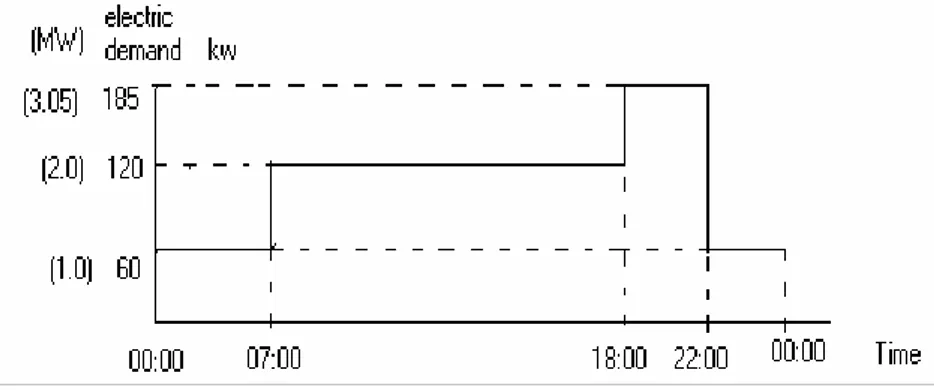
bracketed data are in MW and for 14-Bus system, whereas non-bracketed data are in kW and for 6-Bus system. The following points are considered in the studies
•
Loads as per profiles;•
Zero slack bus injection constraint helps to know, at the planning stage, what exact DER capacity of micro-grid required to meet the internal demand. It is islanded operation of microgrid•
LSI at the terminal buses are usually found higher values, but due to line outage probability, there is a chance of islanding of DERs. At terminal buses these DERs are under utilized. So they are shifted from terminal buses to next higher values.•
Utility is considered as a large virtual generator connected to the microgrid at Bus no. 1, which is slack bus presently. Bus 1 is infinite bus.The data used in two case studies are as follows:
•
Price of utility electricity (Ce) is $ 0.12 /kWh, [14, 16]•
DE data: - Strategy used is DE/rand/1 with per-vector-dither, Population size =20, Scaling factor, or, constant of Differentiation (F) = 0.85; Crossover constant, or, constant of Recombination (Cr) =1;•
PSO data: - Population size: 20; Acceleration Constants: C1, C2 = 2; Generation or iteration = 1000; Inertia weight factor:wmax
=0.95 andwmin
=0.2. Constriction Factor = 1.[15-16]Figure 1. Electric demand profile
5.1 Base case i.e. without DER
6-bus Radial system
The system is shown in Figure 2, where dotted lines indicate co-ordination among central controller (CC), loads controller (LC) and DERs controller (GC). Line data and bus data are shown in Table 1 and Table 2 respectively. Load flow results are shown in Table 4. System loss at peak demand of 185 kW is obtained as 12.2 kW, which is 6.59% of peak demand.
Like consumer demand loss is considered as the system demand to be supplied by the utility’s generators. Therefore, its monetary value could be evaluated by utility’s energy price of $0.12/kwh. Daily energy lost due to line loss is 110.7 kWh and in terms of money $ 13.284.
14-bus system
Bus data and line data are shown in Table 2 and Table 3 respectively. Load flow results are shown in Table 4. System loss at peak demand of 3.05 MW is obtained as 293.3 kW, which is 9.62% of peak demand. Daily energy lost due to line loss is 2530.6 kWh and its monetary value is found 303.672 using the utility’s energy price of $0.12/kwh.
Table 1. Line data
Line No. Start Bus End Bus R [p.u.] X [p.u.] B [p.u.]
Figure 2. 6-bus radial micro-grid
Table 2. Bus Data
6-Bus System 14- Bus system Bus No.
Real load demand, [kW]
Reactive load demand, [kvar]
Real load demand, [kW]
Reactive load demand, [kvar]
1 0.0 0.0 0.0 0.0
2 20.0 6.5 200.0 65.0
3 85.0 27.9 850.0 279
4 40.0 13.12 400.0 131.2
5 20.0 6.5 200.0 65.0
6 20.0 6.5 200.0 65.0
7 - - 76.0 16.0
8 - - 100.0 30.0
9 - - 61.0 16.0
10 - - 112.0 75.0
11 - - 610.0 90.0
12 - - 16.0 61.0
13 - - 90.0 59.0
14 - - 135.0 61.0
Table 3. Line data
Line no. Start Bus End Bus R [p.u.] X [p.u.] B [p.u.]
1 1 2 0.011 0.0214 0.0045
2 2 3 0.011 0.0214 0.0042
3 3 4 0.0115 0.02211 0.0064
4 4 5 0.0127 0.0645 0.0
5 5 6 0.01538 0.05417 0.0
6 6 7 0.0224 0.092 0.0
7 6 8 0.03181 0.0545 0.0
8 7 9 0.0342 0.0917 0.0
Table 4. Base case (5.1)
System Load, kW Line Loss, kW
Minimum Bus Voltage, p.u.
Maximum Line Flow, kW
Slack Bus Injection, kw 185 12.2 0.8362 197.2 197.2 120 4.76 0.9053 128.06 128.06 6-Bus Radial
60 1.06 0.9605 62.56 62.56 3050 293.3 0.8085 3341.4 3341.4 2000 100 0.8974 1990.0 1990.0 14-Bus Radial
1000 28.6 0.9536 1035.8 1035.8
5.2 Strategically deployed DERs
6-bus system
As per LSI data (Figure 3), buses 3 and 4 have highest index value of –0.1424 and –0.3494, but buses 3 and 5 are selected for DERs locations, as per reason given earlier. Terminal bus 4 is swapped with 5. In Figure 3, abscissa is shifted downward to accommodate both positive and negative LSI values. Results of simulation with DE are shown in Table 5 and with PSO in Table 6. With strategic deployment of DERs, voltage rise of 15.46%, loss reduction of 59.02%, and 79.41% line flow reduction happen at peak demand with respect to base case value. Due to line loss reduction, daily energy saving will be 78.5 kWh and corresponding monetary saving is $ 9.42 with respect to base case value.
14-bus system
On considerations of both LSI values (Figure 3) and reliability, as discussed earlier, junction bus numbers 2, 6,and 11 are selected as locations of DERs. Simulation results with DE (Table 5) are obtained at zero slack bus injection i.e. islanded condition and with PSO, results are shown in Table 6. Like 6-bus system, deployment of DERs strategically in the 14-Bus microgrid raise voltage by 17.5%, reduce line loss by 92.36% and reduce line flow by 57.16% at peak demand with respect to base case value. Loss reduction indicates that microgrid is almost a “No wires” solution to distribution system. Line flow reduction reduces internal congestion of the system. Again, voltage rise helps to maintain power quality of supply. Figure 4 indicates the voltage obtained with strategic deployment of DERs with respect to base case. Black bars indicate voltage at base case and white bars at DERs deployed case.
Figure 3. LSI Plot (‘o’ for 6-bus, ‘*’ for 14-bus)
5.3 Comparison between DE and PSO
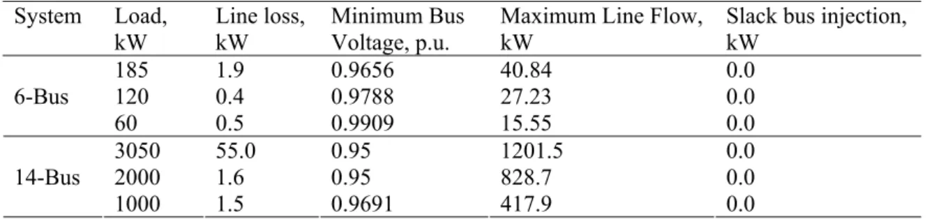
Table 5. Results with DE – case (5.2) System Load, kW Line loss, kW Minimum Bus Voltage, p.u.
Maximum Line Flow, kW
Slack bus injection, kW
185 1.9 0.9656 40.84 0.0 120 0.4 0.9788 27.23 0.0 6-Bus
60 0.5 0.9909 15.55 0.0 3050 55.0 0.95 1201.5 0.0 2000 1.6 0.95 828.7 0.0 14-Bus
1000 1.5 0.9691 417.9 0.0
Table 6. Results with PSO – case (5.2)
System Load, kW Line loss, kW Minimum Bus Voltage, p.u.
Maximum Line Flow, kW
Slack bus injection, kW
185 2.7 0.9656 40.77 0.0 120 0.7 0.9788 27.24 0.0 6-Bus
60 0.5 0.9909 13.45 0.0
3050 75.0 0.95 1207.7 0.0
2000 6.6 0.95 829.0 0.0
14-Bus
1000 2.1 0.9691 417.9 0.0
2 3 4 5 6 7 8 9 10 11 12 13 14 0 0.2 0.4 0.6 0.8 1 1.2 Bus No.---> V o lt ag e, p .u .-- ---->
Comparison between Base case voltage & DERs Deployed Voltage
Figure 4. Voltage histogramfor 14-bus system
Table 7. Results of DE & PSO – case (5.2)
Capacity of DERs at Load, kW System Algorithm Bus No.
Peak Load 2/3rd Peak 1/3rd Peak
Elapsed time for 300 iterations, Secs. 3 107.9 77.7 32.0
DE 5 79.0 46.0 30.0 14.77 3 107.7 83.0 36.0
6-Bus
PSO 5 80.0 41.0 26.0 20.16 2 1300.0 724.1 513.2
6 400.0 392.0 97.1 DE
11 1405.0 915.5 406.2
115.4
2 1300.0 724.1 518.0 6 420.0 397.0 97.8 14-Bus
PSO
11 1405.0 915.5 401.3
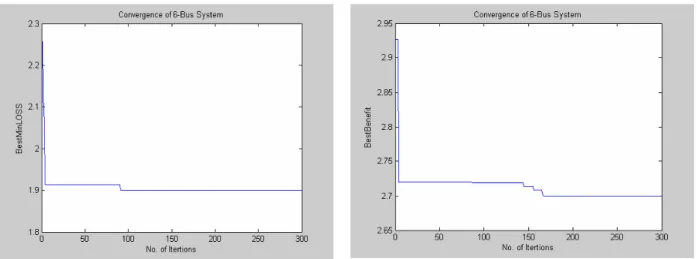
Figure 5. Convergence characteristics of DE – 6-bus system
Figure 6. Convergence characteristics of PSO – 6-bus system
6. Conclusion
Energy management is concerned with cost saving endeavor in microgrid. Strategically deployed DERs have shown reasonable saving of cost in terms of network loss reduction. Owner of the microgrid who are the main instrumental to develop the distribution network and causing such huge saving, must be paid as an incentive for the return of their DERs investment. Voltage rise, line flow reductions are other dominant effect of DERs deployment shown in the results. Future work will be done to analyse microgrid addressing its other benefits. Results of both DE and PSO confirm each other, though DE shows slightly better minimum loss results. What is most attracting to DE is its iteration time much less than PSO.
Acknowledgement
The authors are grateful to the authorities of Electrical Engineering Department of Jadavpur University, India and Electrical Engineering Department, University of Cape Town, South Africa for providing the necessary infrastructure for carrying out this research.
References
[1] Gil, H.A. Joos, G. Models for quantifying the economic benefits of distributed generation. IEEE Trans. on Power Systems, vol. 23, no. 2, pp. 327-335, May 2008.
[2] Harrison, G.P. Piccolo, A. Siano, P. Wallace, A.R. Exploring the tradeoffs between incentives for distributed generation developers and DNOs.IEEE Trans. on Power Systems, vol. 22, no. 2, pp. 821-828, May 2007.
[3] Hatziargyriou, N. Asano, H. Iravani, R. Marnay, C. Microgrids. IEEE Power & Energy Magazine, July / august 2007.
[4] Kueck, J. D. Staunton, R.H. Labinov, S.D. Kirby, B.J. Micro grid energy management. CERTS, Jan. 2003.
[5] Jiayi H. Chuanwen J. Rong X. A review on distributed energy resources and MicroGrid. Renewable & Sustainable Energy Reviews 12 (2008) 247-2483.
[6] Griffin, T. Tomsovic, K. Secrest, D. Law, A. Placement of dispersed generations systems for reduced losses. In Proc. of the 33rd Hawaii International Conf. on System Sciences, 2000.
[7] Greatbanks, J.A. Popovic, D.H. Begovic, M. Pregelj, A. Green, T.C. On optimization for security and reliability of power systems with distributed generation. In Proc. of IEEE Bologna PowerTech Conf., June 23-26, Bologna, Italy.
[8] Nara, K. Hayashi, Y. Ikeda, K. Ashizawa, T. Application of tabu search to optimal placement of distributed generators. In Proc. pf IEEE PES Winter Meeting, vol. 2 pp. 918-923, 2001.
[9] Abdelaziz, A. Ali, W.M. Dispersed generation planning using a new evolutionary approach. In Proc. of IEEE Bologna PowerTech Conf., June 23-26, Bologna, Italy.
[11] Storn, R. Price, K.: Differential evolution- a simple and efficient adaptive scheme for global optimisation over continuous spaces. Technical Report TR-95-012, International Computer Science Institute, Berkley, CA, March 1995.
[12] Price, K.: Differential Evolution: a fast and simple numerical optimiser. Biennial Conference of the North American Fuzzy Information Processing Scoeity, NAFIPS, 19-22 June 1996, pp. 524-527.
[13] Kenedy, J. Eberhart, R. C. Particle Swarm Optimisation. Proceeding of IEEE International Conference on Neural Network (ICNN 1995), vol. 4, Perth, Australia, 1995 pp. 1942-1948.
[14] California Distributed Energy Resource Guide, California Energy Commission, CA, 2004. [on line] http://www.energy.ca.gov/distgen/
[15] Basu, A. K. Bhattacharya, A. Chowdhury, S.P. Chowdhury, S.: Reliability study of a micro-grid system with optimal sizing and placement of DER. Smart Grids for Distribution, IET-CIRED.
CIRED Seminar 23-24 June, pp. 1-4, 2008.
[16] Basu, A.K. Chowdhury, S. Chowdhury, S.P. Strategic deployment of CHP-based distributed energy resources in microgrids. Power and Energy Society General Meeting 2009, PES’09 IEEE, pp. 1-6, 26-30 July 2009.
Ashoke Kumar Basu received his M.Tech. degree in Energy Science & Technology from Jadavpur
University, Kolkata, India in the year 2000 and is working towards his PhD at Jadavpur University, Kolkata, India.. His research interest is micro-grid and he has published six international conference papers, which include IEEE PESGM, CIRED, UPEC etc.
Mr. Basu is a Life Member of Institute of Engineers (India). E-mail address: [email protected]
S.Chowdhury received her BEE and PhD in 1991 and 1998 respectively. She is currently the Senior
Research Officer in the Electrical Engineering Department of The University of Cape Town, South Africa. She became Member of IEEE in 2003. She visited Brunel University, UK and The University of Manchester, UK several times on collaborative research programme. She has published two books and over 55 papers mainly in power systems. She is a Member of the IET (UK) and IE(I) and Member of IEEE(USA). She is acting as YM Coordinator in Indian Network of the IET (UK).
E-mail address: [email protected]
S.P.Chowdhury received his BEE, MEE and PhD in 1987, 1989 and 1992 respectively. In 1993, he joined
E.E.Deptt. of Jadavpur University, Kolkata, India as Lecturer and served till 2008 in the capacity of Professor. He is currently Associate Professor in Electrical Engineering Department in the University of Cape Town, South Africa. He became IEEE Member in 2003. He visited Brunel University, UK and The University of Manchester, UK several times on collaborative research programme. He has published two books and over 110 papers mainly in power systems and renewable energy. He is a fellow of the IET (UK) with C.Eng. IE (I) and the IETE (I) and Member of IEEE (USA). He is a member of technical Professional Service Board of the IET (UK)