Ancestral Reconstruction.

TOPIC PAGE

Ancestral Reconstruction

Jeffrey B. Joy1,2, Richard H. Liang1, Rosemary M. McCloskey1, T. Nguyen1, Art F. Y. Poon1,2*

1BC Centre for Excellence in HIV/AIDS, Vancouver, British Columbia, Canada,2University of British Columbia, Department of Medicine, Vancouver, British Columbia, Canada

*apoon@cfenet.ubc.ca

Introduction

Ancestral reconstruction is the extrapolation back in time from measured characteristics of individuals (or populations) to theircommon ancestors. It is an important application of phylogenetics, the reconstruction and study of theevolutionaryrelationships among individu-als, populations, orspeciesto their ancestors. In the context ofbiology, ancestral reconstruction can be used to recover different kinds of ancestral character states, including thegenetic sequence(ancestral sequence reconstruction), theamino acid sequenceof aprotein, the com-position of agenome(e.g., gene order), a measurable characteristic of an organism (pheno-type), and thegeographic rangeof an ancestral population or species (ancestral range reconstruction). Nonbiological applications include the reconstruction of the vocabulary or phonemes ofancient languages[1] and cultural characteristics of ancient societies such as oral traditions [2] or marriage practices [3].

Ancestral reconstruction relies on a sufficiently realisticmodel of evolutionto accurately recover ancestral states. No matter how well the model approximates the actual evolutionary history, however, one's ability to accurately reconstruct an ancestor deteriorates with increasing evolutionary time between that ancestor and its observed descendants. Additionally, more real-istic models of evolution are inevitably more complex and difficult to calculate. Progress in the field of ancestral reconstruction has relied heavily on theexponential growth of computing powerand the concomitant development of efficientcomputational algorithms(e.g., a dynamic programmingalgorithm for the jointmaximum likelihood[ML] reconstruction of ancestral sequences [4]). Methods of ancestral reconstruction are often applied to a given phylogenetic treethat has already been inferred from the same data. While convenient, this approach has the disadvantage that its results are contingent on the accuracy of a single phylo-genetic tree. In contrast, some researchers advocate a more computationally intensiveBayesian approach that accounts for uncertainty in tree reconstruction by evaluating ancestral recon-structions over many trees [5].

History

The concept of ancestral reconstruction is often credited toEmile ZuckerkandlandLinus Pauling. Motivated by the development of techniques for determining theprimary (amino acid) sequenceof proteins byFrederick Sangerin 1955 [6], Pauling and Zuckerkandl postu-lated [7] that such sequences could be used to infer not only the phylogeny relating the observed protein sequences but also the ancestral protein sequence at the earliest point (root) of this tree. However, the idea of reconstructing ancestors from measurable biological charac-teristics had already been developing in the field ofcladistics, one of the precursors of modern

a11111

OPEN ACCESS

Citation:Joy JB, Liang RH, McCloskey RM, Nguyen T, Poon AFY (2016) Ancestral Reconstruction. PLoS Comput Biol 12(7): e1004763. doi:10.1371/journal. pcbi.1004763

Published:July 12, 2016

Copyright:© 2016 Joy et al. This is an open access article distributed under the terms of theCreative Commons Attribution License, which permits unrestricted use, distribution, and reproduction in any medium, provided the original author and source are credited.

phylogenetics. Cladistic methods, which appeared as early as 1901, infer the evolutionary rela-tionships of species on the basis of the distribution of shared characteristics, of which some are inferred to be descended from common ancestors. Furthermore,Theodoseus Dobzhanskyand Alfred Sturtevantarticulated the principles of ancestral reconstruction in a phylogenetic con-text in 1938, when inferring the evolutionary history ofchromosomal inversionsinDrosophila pseudoobscura[8]. Thus, ancestral reconstruction has its roots in several disciplines. Today, computational methods for ancestral reconstruction continue to be extended and applied in a diversity of settings so that ancestral states are being inferred not only for biological character-istics and the molecular sequences but also for the structure of folded proteins [9,10], the geo-graphic location of populations and species (phylogeography) [11,12], and the higher-order structure of genomes [13].

Methods and Algorithms

Any attempt at ancestral reconstruction begins with aphylogeny. In general, a phylogeny is a tree-basedhypothesisabout the order in which populations (referred to astaxa) are related by descent from common ancestors. Observed taxa are represented by the tips or terminal nodes of the tree that are progressively connected by branches to their common ancestors, which are represented by the branching points of the tree that are usually referred to as the ancestral or internal nodes. Eventually, all lineages converge to themost recent common ancestorof the entire sample of taxa. In the context of ancestral reconstruction, a phylogeny is often treated as though it were a known quantity (with Bayesian approaches being an important exception). Because there can be an enormous number of phylogenies that are nearly equally effective at explaining the data, reducing the subset of phylogenies supported by the data to a single repre-sentative, or point estimate, can be a convenient and sometimes necessary simplifying assump-tion. Ancestral reconstruction can be thought of as the direct result of applying a hypothetical model of evolution to a given phylogeny. When the model contains one or more free parame-ters, the overall objective is to estimate these parameters on the basis of measured characteris-tics among the observed taxa (sequences) that descended from common ancestors.Parsimony is an important exception to this paradigm: though it has been shown that there are mathemat-ical models for which it is the ML estimator [14], at its core, it is simply based on the heuristic that changes in character state are rare, without attempting to quantify that rarity.

Maximum Parsimony

Parsimony, known colloquially as "Occam's razor," refers to the principle of selecting the sim-plest of competing hypotheses. In the context of ancestral reconstruction, parsimony endeavors to find the distribution of ancestral states within a given tree that minimizes the total number of character state changes that would be necessary to explain the states observed at the tips of the tree. This method ofmaximum parsimony) [15] is one of the earliest formalized algorithms for reconstructing ancestral states. Maximum parsimony can be implemented by one of several algorithms. One of the earliest examples isFitch's method[16], which assigns ancestral charac-ter states by parsimony via two traversals of arooted binary tree. The first stage is apostorder traversalthat proceeds from the tips toward the root of a tree by visiting descendant (child) nodes before their parents. Initially, we are determining the set of possible character statesSi for thei-th ancestor based on the observed character states of its descendants. Each assignment is theset intersection) of the character states of the ancestor's descendants; if the intersection is the empty set, then it is theset union). In the latter case, it is implied that a character state change has occurred between the ancestor and one of its two immediate descendants. Each such event counts towards the algorithm's cost function, which may be used to discriminate

Competing Interests:The authors have declared that no competing interests exist.

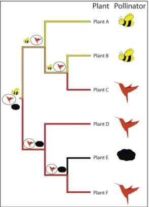
among alternative trees on the basis of maximum parsimony. Next, apreorder traversalof the tree is performed, proceeding from the root towards the tips. Character states are then assigned to each descendant based on which character states it shares with its parent. Since the root has no parent node, one may be required to select a character state arbitrarily, specifically when more than one possible state has been reconstructed at the root. For example, consider a phy-logeny recovered for a genus of plants containing six species, A–F (Fig 1), where each plant is pollinated by either a "bee," "hummingbird," or "wind." One obvious question is what the polli-nators at deeper nodes were in the phylogeny of this genus of plants. Under maximum parsi-mony, an ancestral state reconstruction for this clade reveals that "hummingbird" is the most parsimonious ancestral state for the lower clade (plants D, E, F), that the ancestral states for the nodes in the top clade (plants A, B, C) are equivocal, and that both "hummingbird" or "bee" pollinators are equally plausible for the pollination state at the root of the phylogeny, supposing we have strong evidence from the fossil record that the root state is "hummingbird." Resolution of the root to "hummingbird" would yield the pattern of ancestral state reconstruction depicted by the symbols at the nodes (Fig 1) with the state requiring the fewest number of changes cir-cled. Parsimony methods are intuitively appealing and highly efficient, such that they are still used in some cases to seed ML optimization algorithms with an initial phylogeny [17]. How-ever, they suffer from several issues:

Fig 1. Phylogeny of a hypothetical genus of plants with pollination states of either“bees”, “hummingbirds”, or“wind”denoted by pictues at the tips.Pollination state nodes in the phylogenetic tree inferred under maximum parsimony are coloured on the branches leading into them (yellow represents

“bee”pollination, red representing“hummingbird”pollination, and black representing“wind”pollination, dual coloured branches are equally parsimonious for the two states coloured). Assignment of“hummingbird”as the root state (because of prior knowledge from the fossil record) leads to the pattern of ancestral states represented by symbols at the nodes of the phylogeny, the state requiring the fewest number of changes to give rise to the pattern observed at the tips is circled at each node.

1. Variation in rates of evolution. Fitch's method assumes that changes between all character states are equally likely to occur; thus, any change incurs the same cost for a given tree. This assumption is often unrealistic and can limit the accuracy of such methods. For example, transitions) tend to occur more often thantransversionsin the evolution of nucleic acids. This assumption can be relaxed by assigning differential costs to specific character state changes, resulting in a weighted parsimony algorithm [18].

2. Rapid evolution. The upshot of the "minimum evolution" heuristic underlying such meth-ods is that such methmeth-ods assume that changes are rare and thus are inappropriate in cases where change is the norm rather than the exception [19,20].

3. Variation in time among lineages. Parsimony methods implicitly assume that the same amount of evolutionary time has passed along every branch of the tree. Thus, they do not account for variation in branch lengths in the tree, which are often used to quantify the pas-sage of evolutionary or chronological time. This limitation makes the technique liable to infer that one change occurred on a very short branch rather than multiple changes occur-ring on a very long branch, for example [21]. This shortcoming is addressed by model-based methods (both ML and Bayesian methods) that infer the stochastic process of evolu-tion as it unfolds along each branch of a tree [22].

4. Statistical justification. Without a statistical model underlying the method, its estimates do not have well-defined uncertainties [19,21,23].

ML

ML methods of ancestral state reconstruction treat the character states at internal nodes of the tree as parameters and attempt to find the parameter values that maximize the probability of the data (the observed character states) given the hypothesis (a model of evolution and a phy-logeny relating the observed sequences or taxa). Some of the earliest ML approaches to ances-tral reconstruction were developed in the context ofgenetic sequence evolution[24,25]; similar models were also developed for the analogous case of discrete character evolution [26].

These approaches employ the same probabilistic framework as used to infer the phylogenetic tree [27]. In brief, the evolution of a genetic sequence is modelled by a time-reversible continuous timeMarkov process. In the simplest of these, all characters undergo independent state transitions (such as nucleotide substitutions) at a constant rate over time. This basic model is frequently extended to allow different rates on each branch of the tree. In reality, mutation rates may also vary over time (due, for example, to environmental changes); this can be modelled by allowing the rate parameters to evolve along the tree, at the expense of having an increased number of parameters. A model defines transition probabilities from statesitojalong a branch of lengtht(in units of evolu-tionary time). The likelihood of a phylogeny is computed from a nested sum of transition probabili-ties that corresponds to the hierarchical structure of the proposed tree. At each node, the likelihood of its descendants is summed over all possible ancestral character states at that node:

Lx¼ X

Sx2O

PðSxÞ X

Sy2O

PðSyjSx;t_xyÞL_y

X

Sz2O

PðSzjSx;t_xzÞL_z

where we are computing the likelihood of thesubtreerooted at nodexwith direct descendantsy

Marginal and joint likelihood

Rather than compute the overall likelihood for alternative trees, the problem for ancestral reconstruction is to find the combination of character states at each ancestral node with the highest marginal ML. Generally speaking, there are two approaches to this problem. First, one may work upwards from the descendants of a tree to progressively assign the most likely char-acter state to each ancestor taking into consideration only its immediate descendants. This approach is referred to as marginal reconstruction. It is akin to agreedy algorithmthat makes the locally optimal choice at each stage of the optimization problem. While it can be highly effi-cient, it is not guaranteed to attain a globally optimal solution to the problem. Second, one may instead attempt to find the joint combination of ancestral character states throughout the tree that jointly maximizes the likelihood of the data. Thus, this approach is referred to as joint reconstruction. While it is not as rapid as marginal reconstruction, it is also less likely to be caught in the local optima in nonconvex objective functions thatmodern optimization methods and heuristicsare designed to avoid. In the context of ancestral reconstruction, this means that a marginal reconstruction may assign a character state to the immediate ancestor that is locally optimal but deflects the joint distribution of ancestral character states away from the global optimum (for examples, see Pupko and colleagues [4]). Not surprisingly, joint recon-struction is morecomputationally complexthan marginal reconstruction. Nevertheless, effi-cient algorithms for joint reconstruction have been developed with a time complexity that is generally linear with the number of observed taxa or sequences.

ML-based methods of ancestral reconstruction tend to provide greater accuracy than MP methods in the presence of variation in rates of evolution among characters (or across sites in a genome) [28,29]. However, these methods are not yet able to accommodate variation in rates of evolution over time, otherwise known asheterotachy. If the rate of evolution for a specific character accelerates on a branch of the phylogeny, then the amount of evolution that has occurred on that branch will be underestimated for a given length of the branch and assuming a constant rate of evolution for that character. In addition to that, it is difficult to distinguish heterotachy from variation among characters in rates of evolution [30].

Since ML (unlike maximum parsimony) requires the investigator to specify a model of evo-lution, its accuracy may be affected by the use of a grossly incorrect model (model misspecifica-tion). Furthermore, ML can only provide a single reconstruction of character states (what is often referred to as a "point estimate")—when the likelihood surface is highly nonconvex, com-prising multiple peaks (local optima), then a single point estimate cannot provide an adequate representation, and a Bayesian approach may be more suitable.

Bayesian Inference

Bayesian inferenceuses the likelihood of observed data to update the investigator's belief, or prior distribution, to yield theposterior distribution. In the context of ancestral reconstruction, the objective is to infer the posterior probabilities of ancestral character states at each internal node of a given tree. Moreover, one can integrate these probabilities over the posterior distribu-tions over the parameters of the evolutionary model and the space of all possible trees. This can be expressed as an application ofBayes' theorem:

P Sð jD;yÞ ¼

PðDjS;yÞPðSjyÞ

PðDjy_Þ

/PðDjS;yÞPðSjyÞPðyÞ;

both the evolutionary model and the phylogenetic tree.P(D|S,θ_{) is the likelihood of the} observed data that can be computed byFelsenstein's pruning algorithmas given above.P(S|θ₎ is the prior probability of the ancestral states for a given model and tree. Finally,P(D|θ_{) is the} probability of the data for a given model and tree, integrated over all possible ancestral states. We have given two formulations to emphasize the two different applications of Bayes' theorem, which we discuss in the following section.

Empirical and hierarchical Bayes

One of the first implementations of a Bayesian approach to ancestral sequence reconstruction was developed by Yang and colleagues, where the ML estimates of the evolutionary model and tree, respectively, were used to define the prior distributions. Thus, their approach is an exam-ple of anempirical Bayes methodto compute the posterior probabilities of ancestral character states; this method was first implemented in the software package PAML [31]. In terms of the above Bayesian rule formulation, the empirical Bayes method fixes to the empirical estimates of the model and tree obtained from the data, effectively dropping from the posterior likelihood and prior terms of the formula. Moreover, Yang and colleagues [24] used the empirical distri-bution of site patterns (i.e., assignments of nucleotides to tips of the tree) in their alignment of observed nucleotide sequences in the denominator in place of exhaustively computingP(D) over all possible values ofS, givenθ_{. Computationally, the empirical Bayes method is akin to} the ML reconstruction of ancestral states except that, rather than searching for the ML assign-ment of states based on their respective probability distributions at each internal node, the probability distributions themselves are reported directly.

Empirical Bayes methods for ancestral reconstruction require the investigator to assume that the evolutionary model parameters and tree are known without error. When the size or complexity of the data makes this an unrealistic assumption, it may be more prudent to adopt the fully hierarchical Bayesian approach and infer the joint posterior distribution over the ancestral character states, model, and tree [32]. Huelsenbeck and Bollback [32] first proposed a hierarchical Bayes method to ancestral reconstruction by usingMarkov chain Monte Carlo (MCMC) methods to sample ancestral sequences from this joint posterior distribution. A simi-lar approach was also used to reconstruct the evolution of symbiosis with algae in fungal spe-cies (lichenization) [33]. For example, theMetropolis-Hastings algorithmfor MCMC explores the joint posterior distribution by accepting or rejecting parameter assignments on the basis of the ratio of posterior probabilities.

Put simply, the empirical Bayes approach calculates the probabilities of various ancestral states for a specific tree and model of evolution. By expressing the reconstruction of ancestral states as a set of probabilities, one can directly quantify the uncertainty for assigning any partic-ular state to an ancestor. On the other hand, the hierarchical Bayes approach averages these probabilities over all possible trees and models of evolution, in proportion to how likely these trees and models are, given the data that has been observed.

However, whether the hierarchical Bayes method confers a substantial advantage in practice remains controversial [34]. Moreover, this fully Bayesian approach is limited to analyzing rela-tively small numbers of sequences or taxa because the space ofall possible treesrapidly becomes too vast, making it computationally infeasible forchain samplesto converge in a rea-sonable amount of time.

Calibration

generally decays with increasing time, the use of such specimens provides data that are closer to the ancestors being reconstructed and will most likely improve the analysis, especially when rates of character change vary through time. This concept has been validated by an experimen-tal evolutionary study in which replicate populations ofbacteriophage T7were propagated to generate an artificial phylogeny [35]. In revisiting these experimental data, Oakley and Cun-ningham [36] found that maximum parsimony methods were unable to accurately reconstruct the known ancestral state of a continuous character (plaque size); these results were verified by computer simulation. This failure of ancestral reconstruction was attributed to a directional bias in the evolution of plaque size (from large to small plaque diameters) that required the inclusion of "fossilized" samples to address.

Studies of both mammalian carnivores [37] and fishes [38] have demonstrated that, without incorporating fossil data, the reconstructed estimates of ancestral body sizes are unrealistically large. Moreover, Graham Slater and colleagues showed usingCaniform carnivoransthat incor-porating fossil data into prior distributions improved both the Bayesian inference of ancestral states and evolutionary model selection, relative to analyses using only contemporaneous data [39].

Models

Many models have been developed to estimate ancestral states of discrete and continuous char-acters from extant descendants [40]. Such models assume that the evolution of a trait through time may be modelled as a stochastic process. For discrete-valued traits (such as "pollinator type"), this process is typically taken to be aMarkov chain; for continuous-valued traits (such as "brain size"), the process is frequently taken to be aBrownian motionor anOrnstein–

Uhlenbeck process. Using this model as the basis for statistical inference, one can now useML methods orBayesian inferenceto estimate the ancestral states.

Discrete-state models

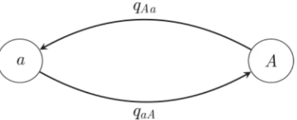
Suppose the trait in question may fall into one ofkstates, labeled 1,. . .,k. The typical means of modelling evolution of this trait is via a continuous-time Markov chain, which may be briefly described as follows (cf.Fig 2). Each state has associated to it rates of transition to all of the other states. The trait is modelled as stepping between thekstates; when it reaches a given state, it starts an exponential "clock" for each of the other states that it can step to. It then "races" the clocks against each other, and it takes a step towards the state whose clock is the first to ring. In such a model, the parameters are the transition ratesq= {qij: 1i,jk,i6¼j},

which can be estimated using, for example, ML methods, where one maximizes over the set of all possible configurations of states of the ancestral nodes.

In order to recover the state of a given ancestral node in the phylogeny (call this nodeα) by

ML, the procedure is: find the ML estimate^qofq; then compute the likelihood of each possible

Fig 2. A general two-state Markov chain representing the rate of jumps from alleleato alleleA.The different types of jumps are allowed to have different rates.

state forαconditioning on_q¼_q^;finally, choose the ancestral state that maximizes this [19].

One may also use this substitution model as the basis for a Bayesian inference procedure, which would consider the posterior belief in the state of an ancestral node given some user-chosen prior.

Because such models may have as many ask(k−1) parameters, overfitting may be an issue. Some common choices that reduce the parameter space are:

• Markovk-state 1 parameter model (Fig 3): this model is the reverse-in-timek-state counter-part of theJukes–Cantormodel. In this model, all transitions have the same rateq, regardless of their start and end states. Some transitions may be disallowed by declaring that their rates are simply 0; this may be the case, for example, if certain states cannot be reached from other states in a single transition.

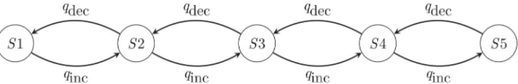
• Asymmetrical Markovk-state 2 parameter model (Fig 4): in this model, the state space is ordered (so that, for example, state 1 is smaller than state 2, which is smaller than state 3, and transitions may only occur between adjacent states). This model contains two parameters

qincandqdec: one for the rate of increase of state (e.g., 0 to 1, 1 to 2, etc.) and one for the rate of decrease in state (e.g., from 2 to 1, 1 to 0, etc.).

Example: Binary state speciation and extinction model

The binary state speciation and extinction model [41] (BiSSE) is a discrete-space model that does not directly follow the framework of those mentioned above. It allows estimation of

Fig 3. Example of a four-state 1 parameter Markov chain model.Note that in this diagram, transitions between statesAandDhave been disallowed; it is conventional to not draw the arrow rather than to draw it with a rate of 0.

doi:10.1371/journal.pcbi.1004763.g003

Fig 4. Graphical representation of an asymmetrical five-state 2-parameter Markov chain model.

ancestral binary character states jointly with diversification rates associated with different char-acter states; it may also be straightforwardly extended to a more general multiple-discrete-state model. In its most basic form, this model involves six parameters: two speciation rates (one each for lineages in states 0 and 1); similarly, two extinction rates; and two rates of character change. This model allows for hypothesis testing on the rates of speciation/extinction/character change, at the cost of increasing the number of parameters.

Continuous-state models

In the case where the trait instead takes nondiscrete values, one must instead turn to a model where the trait evolves as some continuous process. Inference of ancestral states by ML (or by Bayesian methods) would proceed as above but with the likelihoods of transitions in state between adjacent nodes given by some other continuous probability distribution.

• Brownian motion: in this case, if nodesUandVare adjacent in the phylogeny (sayUis the ancestor ofV) and separated by a branch of lengtht, the likelihood of a transition fromU

being in statextoVbeing in stateyis given by a Gaussian density with mean 0 and variance σ2_{t. In this case, there is only one parameter (}σ2_{), and the model assumes that the trait evolves} freely without a bias toward increase or decrease, and that the rate of change is constant throughout the branches of the phylogenetic tree [42].

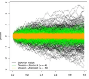
• Ornstein–Uhlenbeck process: in brief, an Ornstein–Uhlenbeck process is a continuous sto-chastic process that behaves like a Brownian motion, but attracted toward some central value, where the strength of the attraction increases with the distance from that value. This is useful for modelling scenarios where the trait is subject to stabilizing selection around a cer-tain value (say 0). Under this model, the above-described transition ofUbeing in statextoV

being in stateywould have a likelihood defined by the transition density of an Ornstein–

Uhlenbeck process with two parameters:σ2_{, which describes the variance of the driving} Brownian motion, andα, which describes the strength of its attraction to 0. Asαtends to 0,

the process is less and less constrained by its attraction to 0 and the process becomes a Brownian motion (Fig 5). Because of this, the models may be nested, and log-likelihood ratio tests discerning which of the two models is appropriate may be carried out.

Fig 5. Plots of 200 trajectories of each of: Brownian motion with drift 0 andσ2= 1 (black); Ornstein– Uhlenbeck withσ2= 1 andα=₋4 (green); and Ornstein–Uhlenbeck withσ2= 1 andα=₋40 (orange).

• Stable models of continuous character evolution [43]: though Brownian motion is appealing and tractable as a model of continuous evolution, it does not permit non-neutrality in its basic form, nor does it provide for any variation in the rate of evolution over time. Instead, one may use astable process, one whose values at fixed times are distributed asstable distributions, to model the evolution of traits. Stable processes, roughly speaking, behave as Brownian motions that also incorporate discontinuous jumps. This allows us to appropri-ately model scenarios in which short bursts of fast trait evolution are expected. In this setting, ML methods are poorly suited because of a rugged likelihood surface and because the likeli-hood may be made arbitrarily large, so Bayesian methods are more appropriate.

Applications

Character evolution

Behaviour and life history evolution. Diet reconstruction in Galapagos finches: Both phy-logenetic and character data are available for the radiation offinchesinhabiting theGalapagos Islands. These data allow testing of hypotheses concerning the timing and ordering of character state changes through time via ancestral state reconstruction. During the dry season, the diets of the 13 species ofGalapagos finchesmay be assorted into three broad diet categories, first those that consume grain-like foods are considered“granivores,”those that ingest arthropods are termed“insectivores,”and those that consume vegetation are classified as“folivores”[19]. Dietary ancestral state reconstruction under maximum parsimony recovers two major shifts from an insectivorous state: one to granivory and one to folivory. Maximum-likelihood ances-tral state reconstruction recovers broadly similar results, with one significant difference: the common ancestor of the tree finch (Camarhynchus) and ground finch (Geospiza) clades is most likely granivorous rather than insectivorous (as judged by parsimony). In this case, this difference between ancestral states returned by maximum parsimony and ML likely occurs as a result of the fact that ML estimates consider branch lengths of the phylogenetic tree [19].

Morphological character evolution mammalian body mass. In an analysis of the body mass of 1,679placental mammalspecies comparing stable models of continuous character evo-lution to Brownian motion models, Elliot and Mooers [43] showed that the evoevo-lutionary pro-cess describing mammalian body mass evolution is best characterized by a stable model of continuous character evolution, which accommodates rare changes of large magnitude. Under a stable model, ancestral mammals retained a low body mass through early diversification, with large increases in body mass coincident with the origin of several orders of large body massed species (e.g., ungulates). By contrast, simulation under a Brownian motion model recovered a less realistic, order of magnitude larger body mass among ancestral mammals, requiring significant reductions in body size prior to the evolution of orders exhibiting small body size (e.g.,Rodentia). Thus, stable models recover a more realistic picture of mammalian body mass evolution by permitting large transformations to occur on a small subset of branches [43].

maximum parsimony by evaluating whether two characters tended to undergo a change on the same branches of the tree [44,45].Felsensteinidentified this problem for continuous character evolution and proposed a solution similar to ancestral reconstruction, in which the phyloge-netic structure of the data was accommodated by directing the analysis on "independent con-trasts" between nodes of the tree related by nonoverlapping branches [23].

Molecular evolution. On a molecular level,amino acid residuesat different locations of a protein may evolve nonindependently, because they have a direct physicochemical interaction, or indirectly by their interactions with a common substrate, or through long-range interactions in the protein structure. Conversely, the folded structure of a protein could potentially be inferred from the distribution of residue interactions [46]. One of the earliest applications of ancestral reconstruction, to predict thethree-dimensional structure of a proteinthrough resi-due contacts, was published by Shindyalov and colleagues [47]. Phylogenies relating 67 differ-ent protein families were generated by a distance-based clustering method (unweighted pair group method with arithmetic mean, UPGMA), and ancestral sequences were reconstructed by parsimony. The authors reported a weak but significant tendency forcoevolvingpairs of res-idues to be colocated in the known three-dimensional structure of the proteins.

More recently, this concept has been applied to identify coevolving residues in protein sequences using more advanced methods for the reconstruction of phylogenies and ancestral sequences. For example, ancestral reconstruction has been used to identify coevolving residues in proteins encoded by RNA virus genomes, particularly in the human immunodeficiency virus (HIV) [48–50].

Vaccine design. RNA viruses such asHIVevolve at an extremely rapid rate, orders of magnitude faster than mammals or birds. For these organisms, ancestral reconstruction can be applied on a much shorter time scale; for example, in order to reconstruct the global or regional progenitor of anepidemicthat has spanned decades rather than millions of years. A team around Brian Gaschen [51] proposed that such reconstructed strains be used as targets for vaccinedesign efforts as opposed to sequences isolated from patients in the present day. Because HIV is extremely diverse, a vaccine designed to work on one patient's viral population might not work for a different patient, because the evolutionary distance between these two viruses may be large. However, their most recent common ancestor is closer to each of the two viruses than they are to each other. Thus, a vaccine designed for a common ancestor could have a better chance of being effective for a larger proportion of circulating strains. Another team took this idea further by developing a center-of-tree (COT) reconstruction method to produce a sequence whose total evolutionary distance to contemporary strains is as small as possible [52]. Strictly speaking, this method was not ancestral reconstruction, as the COT sequence does not necessarily represent a sequence that has ever existed in the evolutionary history of the virus. However, Rolland and colleagues did find that, in the case of HIV, the COT virus was functional when synthesized. Similar experiments with synthetic ancestral sequences obtained by ML reconstruction have likewise shown that these ancestors are both functional and immunogenic, lending some credibility to these methods [53,54]. Furthermore, ancestral reconstruction can potentially be used to infer the genetic sequence of the transmitted HIV variants that have gone on to establish the next infection, with the objective of identifying distinguishing characteristics of these variants (as a nonrandom selection of the transmitted population of viruses) that may be targeted for vaccine design [55].

transposition(a segment is removed from one part of the permutation and spliced in some-where else). The "genome rearrangement problem," first posed by Watterson and colleagues [13], asks: given two genomes (permutations) and a set of allowable operations, what is the shortest sequence of operations that will transform one genome into the other? A generaliza-tion of this problem applicable to ancestral reconstrucgeneraliza-tion is the "multiple genome rearrange-ment problem" [56]: given a set of genomes and a set of allowable operations, find (i) a binary tree with the given genomes as its leaves, and (ii) an assignment of genomes to the internal nodes of the tree, such that the total number of operations across the whole tree is minimized. This approach is similar to parsimony, except that the tree is inferred along with the ancestral sequences. Unfortunately, even the single genome rearrangement problem isNP-hard[57], although it has received much attention in mathematics and computer science (for a review, see Fertin and colleagues [58]).

Spatial applications migration. Ancestral reconstruction is not limited to biological traits. Spatial location is also a trait, and ancestral reconstruction methods can infer the locations of ancestors of the individuals under consideration. Such techniques were used by Lemey and col-leagues to geographically trace the ancestors of 192Avian influenza A-H5N1strains sampled from 20 localities in Europe and Asia and of 101rabies virussequences sampled across 12 Afri-can countries [12].

Treating locations as discrete states (countries, cities, etc.) allows for the application of the discrete-state models described above. However, unlike in a model where the state space for the trait is small, there may be many locations, and transitions between certain pairs of states may rarely or never occur; for example, migration between distant locales may never happen directly if air travel between the two places does not exist, so such migrations must pass through intermediate locales first. This means that there could be many parameters in the model which are zero or close to zero. To this end, Lemey and colleagues used a Bayesian pro-cedure to not only estimate the parameters and ancestral states but also to select which migra-tion parameters are not zero; their work suggests that this procedure does lead to more efficient use of the data. They also explore the use of prior distributions that incorporate geo-graphical structure or hypotheses about migration dynamics, finding that those they consid-ered had little effect on the findings.

Using this analysis, the team around Lemey found that the most likely hub of diffusion of A-H5N1 isGuangdong, withHong Kongalso receiving posterior support. Further, their results support the hypothesis of long-standing presence of African rabies inWest Africa[12].

Species ranges. Inferring historicalbiogeographicpatterns often requires reconstructing ancestral ranges of species on phylogenetic trees [59]. For instance, a well-resolved phylogeny of plant species in the genusCyrtandra[59] was used together with information of their geo-graphic ranges to compare four methods of ancestral range reconstruction. The team com-pared Fitch parsimony [16] (FP; parsimony), stochastic mapping (SM; ML) [60], dispersal-vicariance analysis[61] (DIVA; parsimony), and dispersal-extinction-cladogenesis (DEC; max-imum-likelihood) [11,62]. Results indicated that both parsimony methods performed poorly, which was likely due to the fact that parsimony methods do not consider branch lengths. Both maximum-likelihood methods performed better; however, DEC analyses that additionally allow incorporation of geological priors gave more realistic inferences about range evolution in

Cyrtandrarelative to other methods [59].

higher per-generation dispersal distance in the recently colonized region, a noncentral ances-tral location, and directional migration.

The first consideration of the multiple genome rearrangement problem, long before its for-malization in terms of permutations, was presented by Sturtevant and Dobzhansky in 1936 (Fig 6) [64]. They examined genomes of several strains of fruit fly from different geographic locations, and observed that one configuration, which they called "standard," was the most common throughout all the studied areas. Remarkably, they also noticed that four different strains could be obtained from the standard sequence by a single inversion, and two others could be related by a second inversion. This allowed them to hypothesize a phylogeny for the sequences and to infer that the standard sequence was probably also the ancestral one.

Linguistic evolution. Reconstructions of the words and phenomes of ancient

protolanguagessuch asProto-Indo-Europeanhave been performed based on the observed ana-logues in present-day languages. Typically, these analyses are carried out manually using the "comparative method" [65]. First, words from different languages with a common etymology (cognates) are identified in the contemporary languages under study, analogous to the identifica-tion oforthologousbiological sequences. Second, correspondences between individual sounds in the cognates are identified, a step similar to biologicalsequence alignment, although performed manually. Finally, likely ancestral sounds are hypothesized by manual inspection and various heuristics (such as the fact that most languages have bothnasal and non-nasal vowels) [65].

Software

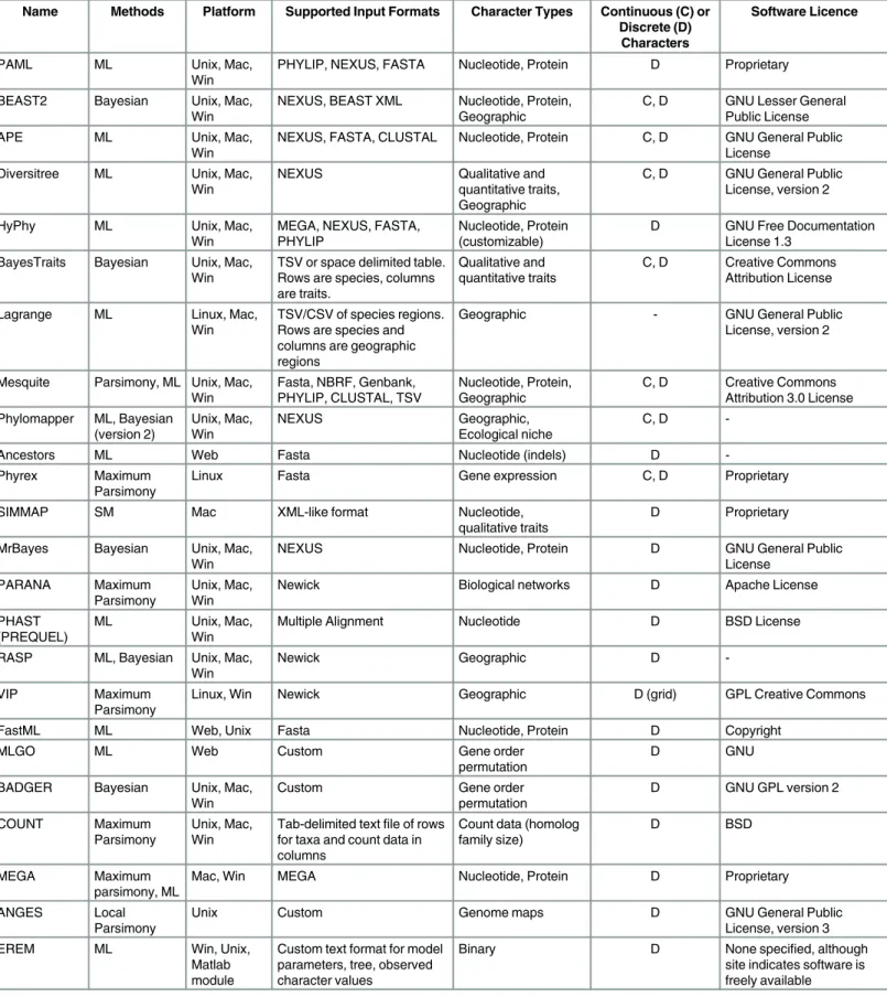
There are many software packages available that perform ancestral state reconstruction. Gener-ally, these software packages have been developed and maintained through the efforts of scien-tists in related fields and released underfree software licenses. The following table is not meant to be a comprehensive itemization of all available packages, but provides a representative sam-ple of the extensive variety of packages that imsam-plement methods of ancestral reconstruction with different strengths and features (Table 1).

Package Descriptions

Molecular evolution

The majority of these software packages are designed for analyzing genetic sequence data. For example, PAML [31] is a collection of programs for the phylogenetic analysis of DNA and

Fig 6. Phylogeny of seven regional strains ofDrosophila pseudoobscura, as inferred by Sturtevant and Dobzhansky [64].Displayed sequences do not correspond to the original paper, but were derived from the notation in the authors' companion paper [8] as follows: A (63A–

65B), B (65C–68D), C (69A–70A), D (70B–70D), E (71A–71B), F (71A–73C), G (74A–74C), H (75A–75C), I (76A–76B), J (76C–77B), K (78A–

79D), L (80A–81D). Inversions inferred by the authors are highlighted in blue along branches.

Table 1. List of software for ancestral reconstruction.

Name Methods Platform Supported Input Formats Character Types Continuous (C) or Discrete (D)

Characters

Software Licence

PAML ML Unix, Mac,

Win

PHYLIP, NEXUS, FASTA Nucleotide, Protein D Proprietary

BEAST2 Bayesian Unix, Mac, Win

NEXUS, BEAST XML Nucleotide, Protein, Geographic

C, D GNU Lesser General Public License

APE ML Unix, Mac,

Win

NEXUS, FASTA, CLUSTAL Nucleotide, Protein C, D GNU General Public License

Diversitree ML Unix, Mac,

Win

NEXUS Qualitative and

quantitative traits, Geographic

C, D GNU General Public License, version 2

HyPhy ML Unix, Mac,

Win

MEGA, NEXUS, FASTA, PHYLIP

Nucleotide, Protein (customizable)

D GNU Free Documentation License 1.3

BayesTraits Bayesian Unix, Mac, Win

TSV or space delimited table. Rows are species, columns are traits.

Qualitative and quantitative traits

C, D Creative Commons Attribution License

Lagrange ML Linux, Mac,

Win

TSV/CSV of species regions. Rows are species and columns are geographic regions

Geographic - GNU General Public

License, version 2

Mesquite Parsimony, ML Unix, Mac, Win

Fasta, NBRF, Genbank, PHYLIP, CLUSTAL, TSV

Nucleotide, Protein, Geographic

C, D Creative Commons Attribution 3.0 License Phylomapper ML, Bayesian

(version 2)

Unix, Mac, Win

NEXUS Geographic,

Ecological niche

C, D

-Ancestors ML Web Fasta Nucleotide (indels) D

-Phyrex Maximum

Parsimony

Linux Fasta Gene expression C, D Proprietary

SIMMAP SM Mac XML-like format Nucleotide,

qualitative traits

D Proprietary

MrBayes Bayesian Unix, Mac, Win

NEXUS Nucleotide, Protein D GNU General Public

License

PARANA Maximum

Parsimony

Unix, Mac, Win

Newick Biological networks D Apache License

PHAST (PREQUEL)

ML Unix, Mac,

Win

Multiple Alignment Nucleotide D BSD License

RASP ML, Bayesian Unix, Mac, Win

Newick Geographic D

-VIP Maximum

Parsimony

Linux, Win Newick Geographic D (grid) GPL Creative Commons

FastML ML Web, Unix Fasta Nucleotide, Protein D Copyright

MLGO ML Web Custom Gene order

permutation

D GNU

BADGER Bayesian Unix, Mac, Win

Custom Gene order

permutation

D GNU GPL version 2

COUNT Maximum

Parsimony

Unix, Mac, Win

Tab-delimited textfile of rows for taxa and count data in columns

Count data (homolog family size)

D BSD

MEGA Maximum

parsimony, ML

Mac, Win MEGA Nucleotide, Protein D Proprietary

ANGES Local

Parsimony

Unix Custom Genome maps D GNU General Public

License, version 3

EREM ML Win, Unix,

Matlab module

Custom text format for model parameters, tree, observed character values

Binary D None specified, although

site indicates software is freely available

protein sequence alignments by ML. Ancestral reconstruction can be performed using the codeml program.HyPhy,Mesquite, andMEGAare also software packages for the phylogenetic analysis of sequence data, but are designed to be more modular and customizable. HyPhy [66] implements a joint ML method of ancestral sequence reconstruction [4] that can be readily adapted to reconstructing a more generalized range of discrete ancestral character states such as geographic locations by specifying a customized model in its batch language. Mesquite [67] provides ancestral state reconstruction methods for both discrete and continuous characters using both maximum parsimony and ML methods. It also provides several visualization tools for interpreting the results of ancestral reconstruction. MEGA [68] is a modular system, too, but places greater emphasis on ease-of-use than customization of analyses. As of version 5, MEGA allows the user to reconstruct ancestral states using maximum parsimony, ML, and empirical Bayes methods [68].

The Bayesian analysis of genetic sequences may confer greater robustness to model misspe-cification. MrBayes [69] allows inference of ancestral states at ancestral nodes using the full hierarchical Bayesian approach. The PREQUEL program distributed in the PHAST package performs comparative evolutionary genomics using ancestral sequence reconstruction [70]. SIMMAP stochastically maps mutations on phylogenies [71]. BayesTraits [26] analyses dis-crete or continuous characters in a Bayesian framework to evaluate models of evolution, recon-struct ancestral states, and detect correlated evolution between pairs of traits.

Other character types. Other software packages are more oriented towards the analysis of qualitative and quantitative traits (phenotypes). For example, the ape package [72] in the statis-tical computing environment R also provides methods for ancestral state reconstruction for both discrete and continuous characters through theacefunction, including ML. Note thatace

performs reconstruction by computing scaled conditional likelihoods instead of the marginal or joint likelihoods used by other ML-based methods for ancestral reconstruction, which may adversely affect the accuracy of reconstruction at nodes other than the root. Phyrex implements a maximum parsimony-based algorithm to reconstruct ancestral gene expression profiles in addition to a ML method for reconstructing ancestral genetic sequences (by wrapping around the baseml function in PAML) [73].

Several software packages also reconstructphylogeography. BEAST (Bayesian Evolutionary Analysis by Sampling Trees [74]) provides tools for reconstructing ancestral geographic loca-tions from observed sequences annotated with location data using Bayesian MCMC sampling methods. Diversitree [75] is an R package providing methods for ancestral state reconstruction under Mk2 (acontinuous time Markov modelof binary character evolution [76]) and BiSSE models. Lagrange performs analyses on reconstruction of geographic range evolution on phy-logenetic trees [11]. Phylomapper [63] is a statistical framework for estimating historical pat-terns of gene flow and ancestral geographic locations. RASP [77] infers ancestral state using statistical DIVA, Lagrange, Bayes-Lagrange, BayArea, and BBM methods. VIP [78] infers his-torical biogeography by examining disjunct geographic distributions.

Genome rearrangements provide valuable information incomparative genomicsbetween species. ANGES [79] compares extant-related genomes through ancestral reconstruction of genetic markers. BADGER [80] uses a Bayesian approach to examining the history of gene rearrangement. Count [81] reconstructs the evolution of the size of gene families. EREM [82] analyses the gain and loss of genetic features encoded by binary characters. PARANA [83] per-forms parsimony-based inference of ancestral biological networks that represent gene loss and duplication.

genome reconstruction by the identification and arrangement ofsyntenicregions. FastML [85] is a web server for probabilistic reconstruction of ancestral sequences by ML that uses a gap character model for reconstructingindelvariation. MLGO [86] is a web server for ML gene order analysis.

Future Directions

The development and application of computational algorithms for ancestral reconstruction continues to be an active area of research across disciplines. For example, the reconstruction of sequence insertions and deletions (indels) has lagged behind the more straightforward applica-tion of substituapplica-tion models. Bouchard-Côté and Jordan recently described a new model (the Poisson Indel Process [87]) that represents an important advance on the archetypal Thorne-Kishino-Felsenstein model of indel evolution [88]. In addition, the field is being driven forward by rapid advances in the area ofnext-generation sequencingtechnology, where sequences are generated from millions of nucleic acid templates by extensive parallelization of sequencing reactions in a custom apparatus. These advances have made it possible to generate a"deep" snapshotof the genetic composition of a rapidly-evolving population, such as RNA viruses [89] or tumour cells [90], in a relatively short amount of time. At the same time, the massive amount of data and platform-specific sequencing error profiles has created new bioinformatic challenges for processing these data for ancestral sequence reconstruction.

The version history of the text file and the peer reviews (and response to reviews) are avail-able as supporting information inS1andS2Texts.

Supporting Information

S2 Text. Peer reviews and response to reviews.Human-readable versions of the reviews and authors' responses are available as comments on this article.

(XML)

References

1. Platnick NI, Cameron HD. Cladistic methods in textual, linguistic, and phylogenetic analysis. System-atic Biology. 1977; 26(4):380–5.

2. Tehrani JJ. The phylogeny of little red riding hood. PloS ONE. 2013; 8(11):e78871. doi:10.1371/ journal.pone.0078871PMID:24236061

3. Walker RS, Hill KR, Flinn MV, Ellsworth RM. Evolutionary history of hunter-gatherer marriage practices. PLoS ONE. 2011; 6(4):e19066. doi:10.1371/journal.pone.0019066PMID:21556360

4. Pupko T, Pe I, Shamir R, Graur D. A fast algorithm for joint reconstruction of ancestral amino acid sequences. Molecular Biology and Evolution. 2000; 17(6):890–6. PMID:10833195

5. Pagel M, Meade A, Barker D. Bayesian Estimation of Ancestral Character States on Phylogenies. Sys-tematic Biology. 2004; 53(5):673–84. PMID:15545248

6. Sanger F, Thompson EOP, Kitai R. The amide groups of insulin. Biochemical Journal. 1955; 59(3):509. PMID:14363129

7. Pauling L, Zuckerkand E. Chemical Paleogenetics: Molecular "Restoration Studies" of Extinct Forms of Life. Acta Chemica Scandinavica. 1963; 17:9–16. doi:10.3891/acta.chem.scand.17s-0009

8. Dobzhansky T, Sturtevant AH. Inversions in the chromosomes of Drosophila pseudoobscura. Genet-ics. 1938; 23(1):28. PMID:17246876

10. Williams PD, Pollock DD, Blackburne BP, Goldstein RA. Assessing the accuracy of ancestral protein reconstruction methods. PLoS Comput Biol. 2006; 2(6):e69. PMID:16789817

11. Ree RH, Smith SA. Maximum likelihood inference of geographic range evolution by dispersal, local extinction, and cladogenesis. Systematic Biology. 2008; 57(1):4–14. doi:10.1080/

10635150701883881PMID:18253896

12. Lemey P, Rambaut A, Drummond AJ, Suchard MA. Bayesian Phylogeography Finds Its Roots. PLoS Comput Biol. 2009; 5.

13. Watterson GA, Ewens WJ, Hall TE, Morgan A. The chromosome inversion problem. Journal of Theoret-ical Biology. 1982; 99(1):1–7.

14. Tuffley C, Steel M. Links between maximum likelihood and maximum parsimony under a simple model of site substitution. Bulletin of mathematical biology. 1997; 59(3):581–607. PMID:9172826

15. Swofford DL, Maddison WP. Reconstructing ancestral character states under Wagner parsimony. Mathematical Biosciences. 1987; 87(2):199–229.

16. Fitch WM. Toward defining the course of evolution: minimum change for a specific tree topology. Sys-tematic Biology. 1971; 20(4):406–16.

17. Stamatakis A. RAxML-VI-HPC: maximum likelihood-based phylogenetic analyses with thousands of taxa and mixed models. Bioinformatics. 2006; 22:2688–90. PMID:16928733

18. Sankoff D. Minimal mutation trees of sequences. SIAM Journal on Applied Mathematics. 1975; 28 (1):35–42.

19. Schluter D, Price T, Mooers AO, Ludwig D. Likelihood of ancestor states in adaptive radiation. Evolu-tion. 1997; 51(6):1699–711. PMID:ISI:000071652200001.

20. Felsenstein J. Maximum likelihood and minimum-steps methods for estimating evolutionary trees from data on discrete characters. Systematic Biology. 1973; 22(3):240–9.

21. Cunningham CW, Omland KE, Oakley TH. Reconstructing ancestral character states: a critical reap-praisal. Trends in Ecology & Evolution. 1998; 13(9):361–6.

22. Li G, Steel M, Zhang L. More taxa are not necessarily better for the reconstruction of ancestral character states. Systematic biology. 2008; 57(4):647–53. doi:10.1080/10635150802203898PMID:18709600

23. Felsenstein J. Phylogenies and the comparative method. American Naturalist. 1985:1–15.

24. Yang Z, Kumar S, Nei M. A new method of inference of ancestral nucleotide and amino acid sequences. Genetics. 1995; 141(4):1641–50. PMID:8601501

25. Koshi JM, Goldstein RA. Probabilistic reconstruction of ancestral protein sequences. Journal of Molec-ular Evolution. 1996; 42(2):313–20. PMID:8919883

26. Pagel M. The maximum likelihood approach to reconstructing ancestral character states of discrete characters on phylogenies. Systematic biology. 1999; 48(3):612–22.

27. Felsenstein J. Evolutionary trees from DNA sequences: a maximum likelihood approach. Journal of molecular evolution. 1981; 17(6):368–76. PMID:7288891

28. Eyre-Walker A. Problems with parsimony in sequences of biased base composition. Journal of Molecu-lar Evolution. 1998; 47(6):686–90. PMID:9847410

29. Pupko T, Pe'er I, Hasegawa M, Graur D, Friedman N. A branch-and-bound algorithm for the inference of ancestral amino-acid sequences when the replacement rate varies among sites: Application to the evolution of five gene families. Bioinformatics. 2002; 18(8):1116–23. PMID:12176835

30. Gruenheit N, Lockhart PJ, Steel M, Martin W. Difficulties in testing for covarion-like properties of sequences under the confounding influence of changing proportions of variable sites. Molecular Biol-ogy and Evolution. 2008; 25(7):1512–20. doi:10.1093/molbev/msn098PMID:18424773

31. Yang Z. PAML 4: phylogenetic analysis by maximum likelihood. Molecular biology and evolution. 2007; 24(8):1586–91. PMID:17483113

32. Huelsenbeck JP, Bollback JP. Empirical and hierarchical Bayesian estimation of ancestral states. Sys-tematic Biology. 2001; 50(3):351–66. PMID:ISI:000169823200006.

33. Lutzoni F, Pagel M, Reeb V. Major fungal lineages are derived from lichen symbiotic ancestors. Nature. 2001; 411(6840):937–40. PMID:11418855

34. Hanson-Smith V, Kolaczkowski B, Thornton JW. Robustness of ancestral sequence reconstruction to phylogenetic uncertainty. Molecular biology and evolution. 2010; 27(9):1988–99. doi:10.1093/molbev/ msq081PMID:20368266

35. Hillis DM, Bull JJ, White ME, Badgett MR, Molineux IJ. Experimental phylogenetics: generation of a known phylogeny. Science. 1992; 255(5044):589–92. PMID:1736360

37. Finarelli JA, Flynn JJ. Ancestral state reconstruction of body size in the Caniformia (Carnivora, Mamma-lia): the effects of incorporating data from the fossil record. Systematic Biology. 2006; 55(2):301–13. PMID:16611601

38. Albert JS, Johnson DM, Knouft JH. Fossils provide better estimates of ancestral body size than do extant taxa in fishes. Acta Zoologica. 2009; 90(s1):357–84.

39. Slater GJ, Harmon LJ, Alfaro ME. Integrating fossils with molecular phylogenies improves inference of trait evolution. Evolution. 2012; 66(12):3931–44. doi:10.1111/j.1558-5646.2012.01723.xPMID: 23206147

40. Webster AJ, Purvis A. Testing the accuracy of methods for reconstructing ancestral states of continu-ous characters. Proceedings of the Royal Society of London B: Biological Sciences. 2002; 269 (1487):143–9.

41. Maddison WP, Midford PE, Otto SP. Estimating a binary character's effect on speciation and extinction. Systematic biology. 2007; 56(5):701–10. PMID:17849325

42. Martins EP. Estimating the rate of phenotypic evolution from comparative data. American Naturalist. 1994:193–209.

43. Elliot MG, Mooers AØ_{. Inferring ancestral states without assuming neutrality or gradualism using a} sta-ble model of continuous character evolution. BMC evolutionary biology. 2014; 14(1):226.

44. Ridley M. The explanation of organic diversity: the comparative method and adaptations for mating. Oxford: Clarendon Press; 1983.

45. Maddison WP. A method for testing the correlated evolution of two binary characters: are gains or losses concentrated on certain branches of a phylogenetic tree? Evolution. 1990:539–57.

46. Göbel U, Sander C, Schneider R, Valencia A. Correlated mutations and residue contacts in proteins. Proteins: Structure, Function, and Bioinformatics. 1994; 18(4):309–17.

47. Shindyalov IN, Kolchanov NA, Sander C. Can three-dimensional contacts in protein structures be pre-dicted by analysis of correlated mutations? Protein Engineering. 1994; 7(3):349–58. PMID:8177884

48. Korber BT, Farber RM, Wolpert DH, Lapedes AS. Covariation of mutations in the V3 loop of human immunodeficiency virus type 1 envelope protein: an information theoretic analysis. Proceedings of the National Academy of Sciences. 1993; 90(15):7176–80.

49. Shapiro B, Rambaut A, Pybus OG, Holmes EC. A phylogenetic method for detecting positive epistasis in gene sequences and its application to RNA virus evolution. Molecular biology and evolution. 2006; 23(9):1724–30. PMID:16774976

50. Poon AFY, Lewis FI, Pond SLK, Frost SDW. An evolutionary-network model reveals stratified interac-tions in the V3 loop of the HIV-1 envelope. PLoS Comput Biol. 2007; 3(11):e231. PMID:18039027

51. Gaschen B, Taylor J, Yusim K, Foley B, Gao F, Lang D, et al. Diversity considerations in HIV-1 vaccine selection. Science. 2002; 296(5577):2354–60. PMID:12089434

52. Rolland M, Jensen MA, Nickle DC, Yan J, Learn GH, Heath L, et al. Reconstruction and function of ancestral center-of-tree human immunodeficiency virus type 1 proteins. Journal of virology. 2007; 81 (16):8507–14. PMID:17537854

53. Kothe DL, Li Y, Decker JM, Bibollet-Ruche F, Zammit KP, Salazar MG, et al. Ancestral and consensus envelope immunogens for HIV-1 subtype C. Virology. 2006; 352(2):438–49. PMID:16780913

54. Doria-Rose NA, Learn GH, Rodrigo AG, Nickle DC, Li F, Mahalanabis M, et al. Human immunodefi-ciency virus type 1 subtype B ancestral envelope protein is functional and elicits neutralizing antibodies in rabbits similar to those elicited by a circulating subtype B envelope. Journal of virology. 2005; 79 (17):11214–24. PMID:16103173

55. McCloskey RM, Liang RH, Harrigan PR, Brumme ZL, Poon AFY. An evaluation of phylogenetic meth-ods for reconstructing transmitted HIV variants using longitudinal clonal HIV sequence data. Journal of virology. 2014; 88(11):6181–94. doi:10.1128/JVI.00483-14PMID:24648453

56. Bourque G, Pevzner PA. Genome-scale evolution: reconstructing gene orders in the ancestral species. Genome research. 2002; 12(1):26–36. PMID:11779828

57. Even S, Goldreich O. The minimum-length generator sequence problem is NP-hard. Journal of Algo-rithms. 1981; 2(3):311–3.

58. Fertin G. Combinatorics of genome rearrangements: MIT press; 2009.

59. Clark JR, Ree RH, Alfaro ME, King MG, Wagner WL, Roalson EH. A comparative study in ancestral range reconstruction methods: retracing the uncertain histories of insular lineages. Systematic Biology. 2008; 57(5):693–707. doi:10.1080/10635150802426473PMID:18853357

61. Ronquist F. DIVA version 1.2. Computer program for MacOS and Win32. Evolutionary Biology Centre, Uppsala University Available athttp://www.ebcuuse/systzoo/research/diva/divahtml. 2001.

62. Ree RH, Moore BR, Webb CO, Donoghue MJ. A likelihood framework for inferring the evolution of geo-graphic range on phylogenetic trees. Evolution. 2005; 59(11):2299–311. PMID:16396171

63. Lemmon AR, Lemmon EM. A likelihood framework for estimating phylogeographic history on a continu-ous landscape. Systematic Biology. 2008; 57(4):544–61. doi:10.1080/10635150802304761PMID: 18686193

64. Sturtevant AH, Dobzhansky T. Geographical Distribution and Cytology of" Sex Ratio" in Drosophila Pseudoobscura and Related Species. Genetics. 1936; 21(4):473. PMID:17246805

65. Campbell L. Historical linguistics: Edinburgh University Press; 2013.

66. Pond SLK, Muse SV. HyPhy: hypothesis testing using phylogenies. Statistical methods in molecular evolution: Springer; 2005. p. 125–81.

67. Maddison W, Maddison D. Mesquite: a modular system for evolutionary analysis. 2.75 ed20011.

68. Tamura K, Dudley J, Nei M, Kumar S. MEGA4: molecular evolutionary genetics analysis (MEGA) soft-ware version 4.0. Molecular biology and evolution. 2007; 24(8):1596–9. PMID:17488738

69. Huelsenbeck JP, Ronquist F. MRBAYES: Bayesian inference of phylogenetic trees. Bioinformatics. 2001; 17(8):754–5. PMID:ISI:000171021000016.

70. Hubisz MJ, Pollard KS, Siepel A. PHAST and RPHAST: phylogenetic analysis with space/time models. Briefings in bioinformatics. 2011; 12(1):41–51. doi:10.1093/bib/bbq072PMID:21278375

71. Bollback JP. SIMMAP: stochastic character mapping of discrete traits on phylogenies. BMC bioinfor-matics. 2006; 7(1):88.

72. Paradis E. Analysis of phylogenetics and evolution with R. New York: Springer; 2006.

73. Rossnes R, Eidhammer I, Liberles DA. Phylogenetic reconstruction of ancestral character states for gene expression and mRNA splicing data. BMC bioinformatics. 2005; 6(1):127.

74. Bouckaert R, Heled J, Kühnert D, Vaughan T, Wu C- H, Xie D, et al. BEAST 2: a software platform for Bayesian evolutionary analysis. PLoS Comput Biol. 2014; 10(4):e1003537. doi:10.1371/journal.pcbi. 1003537PMID:24722319

75. FitzJohn RG. Diversitree: comparative phylogenetic analyses of diversification in R. Methods in Ecol-ogy and Evolution. 2012; 3(6):1084–92.

76. Pagel M. Detecting Correlated Evolution on Phylogenies—a General- Method for the Comparative-Analysis of Discrete Characters. Proceedings of the Royal Society of London Series B-Biological Sci-ences. 1994; 255(1342):37–45. PMID:ISI:A1994MT55500006.

77. Yu Y, Harris AJ, Blair C, He X. RASP (Reconstruct Ancestral State in Phylogenies): a tool for historical biogeography. Molecular Phylogenetics and Evolution. 2015; 87:46–9. doi:10.1016/j.ympev.2015.03. 008PMID:25819445

78. Arias JS, Szumik CA, Goloboff PA. Spatial analysis of vicariance: a method for using direct geographi-cal information in historigeographi-cal biogeography. Cladistics. 2011; 27(6):617–28.

79. Jones BR, Rajaraman A, Tannier E, Chauve C. ANGES: reconstructing ANcestral GEnomeS maps. Bioinformatics. 2012; 28(18):2388–90. doi:10.1093/bioinformatics/bts457PMID:22820205

80. Larget B, Kadane JB, Simon DL. A Bayesian approach to the estimation of ancestral genome arrange-ments. Molecular phylogenetics and evolution. 2005; 36(2):214–23. PMID:15893477

81. Csű_{ös M. Count: evolutionary analysis of phylogenetic profiles with parsimony and likelihood.}

Bioinfor-matics. 2010; 26(15):1910–2. doi:10.1093/bioinformatics/btq315PMID:20551134

82. Affre L, Thompson JD, Debussche M. Genetic structure of continental and island populations of the Mediterranean endemic Cyclamen balearicum (Primulaceae). American Journal of Botany. 1997; 84 (4):437–51. PMID:ISI:A1997WV34000002.

83. Patro R, Sefer E, Malin J, Marçais G, Navlakha S, Kingsford C. Parsimonious reconstruction of network evolution. Algorithms for Molecular Biology. 2012; 7(1):1.

84. Diallo AB, Makarenkov V, Blanchette M. Ancestors 1.0: a web server for ancestral sequence recon-struction. Bioinformatics. 2010; 26(1):130–1. doi:10.1093/bioinformatics/btp600PMID:19850756

85. Ashkenazy H, Penn O, Doron-Faigenboim A, Cohen O, Cannarozzi G, Zomer O, et al. FastML: a web server for probabilistic reconstruction of ancestral sequences. Nucleic acids research. 2012; 40(W1): W580–W4.

86. Hu F, Lin Y, Tang J. MLGO: phylogeny reconstruction and ancestral inference from gene-order data. BMC bioinformatics. 2014; 15(1):1.

88. Thorne JL, Kishino H, Felsenstein J. An evolutionary model for maximum likelihood alignment of DNA sequences. Journal of Molecular Evolution. 1991; 33(2):114–24. PMID:1920447

89. Poon AFY, Swenson LC, Bunnik EM, Edo-Matas D, Schuitemaker H, van't Wout AB, et al. Reconstruct-ing the dynamics of HIV evolution within hosts from serial deep sequence data. PLoS Comput Biol. 2012; 8(11):e1002753. doi:10.1371/journal.pcbi.1002753PMID:23133358