Influences of surface temperature on a low camber airfoil aerodynamic performances

(1)

Influences of surface temperature on a low camber airfoil

aerodynamic performances

Valeriu DRAGAN*

*Corresponding author

INCDT COMOTI - National Institute for Gas Turbines

B-dul Iuliu Maniu 220 D, Bucharest 061126, Romania

drvaleriu@gmail.com

DOI: 10.13111/2066-8201.2016.8.1.6 Received: 22 January 2016/ Accepted: 07 February 2016

Abstract: The current note refers to the comparison between a NACA 2510 airfoil with adiabatic walls and the same airfoil with heated patches. Both suction and pressure sides were divided into two regions covering the leading edge (L.E.) and trailing edge (T.E.). A RANS method sensitivity test has been performed in the preliminary stage while for the extended 3D cases a DES-SST approach was used. Results indicate that surface temperature distribution influences the aerodynamics of the airfoil, in particular the viscous drag component but also the lift of the airfoil. Moreover, the influence depends not only on the surface temperature but also on the positioning of the heated surfaces, particularly in the case of pressure lift and drag. Further work will be needed to optimize the temperature distribution for airfoil with higher camber.

Key Words: RANS, DES, thermal boundary layer, airfoil thermal trimming

1. INTRODUCTION



Thermal influences on both laminar and turbulent boundary layer have been studied for a long time both experimentally [1-3] and numerically [4-7].

Typical tests on airfoils have been performed on low speed, long chord airfoils for aircraft wing de-icing [8]. The expected conclusions of the experimental tests were that the heated leading edge has a detrimental effect on the lift and drag performance of the wing. However, this does not necessarily apply to airfoils operating on lower Reynolds numbers [9] where viscous drag dominates.

Typically, the Reynolds number varies inversely proportionate to the temperature of the flow.

However, the case where the flow is only locally heated in the viscous sub-layer of the boundary layer, this in not necessarily an impediment.

As it will become apparent, the local Reynolds number as well as wall shear stress and skin friction coefficient (which are all linked) do decrease.

In spite of this, the traditional wisdom that the lift to drag ratio is proportionate to the Reynolds number, in the heated cases improvements have been observed after Detached Eddy Simulations.

(2)

2. PROBLEM FORMULATION

Due to the high complexity of the problem which will be studied, i.e. the interaction between the thermal and the velocity boundary layer, two levels of accuracy were considered. Thusly, in the initial phase, a 2D series of CFD simulations were carried out with the purpose of investigating the modeling accuracy of various RANS methods and also to test the merits of the idea that the aerodynamic coefficients can be altered through thermal effects on the walls. Following this preliminary test, two more 3D cases were studied, considering a narrow strip and a wide strip with lateral symmetry conditions.

2.1 The preliminary tests - 2D CFD

The cases studied in the hereby note refer to a NACA 2510 airfoil with a chord of 0.35 m in 2D as well as in simple 3D cases with periodic conditions, one of which has a width of 0.7 m. Endwall effects have not been studied due in part to the computational effort implied by a larger domain and also in order to isolate the influence of heat transfer on the airfoil from other phenomena such as tip vortex formation.

Four patches were considered, covering pressure and suction side and leading and trailing edges. The cutting point for the suction (top) surface is located at 0.1 m and the cutting point for the pressure side (bottom) is located at 0.0775 m in the Ox direction.

Since the operating speed of the wing itself varies considerably, a proper method to test the usefulness of this method would imply a fixed available power to be exchanged between the wing and the ambient air. However, since the available power value depends very much on the heat source - which has yet to be established - a constant temperature value was set for the heated surface. Also, a fixed 50 m/s velocity was chosen for all presented cases.

It is to be expected that, since heat transfer is proportional with air speed, at lower relative velocities the heated wing will have an exacerbated behavior whereas at higher relative speeds, the effects should become negligible. Another influence on the effectiveness of the heated wing is the Reynolds number change with airspeed - which influences the local Nusselt number as well as the proportion of viscous drag, hence theoretically the impact at low speeds should be more beneficial.

For the initial analysis, a steady state RANS model approach was used. Two turbulence models were selected in the preliminary stage, namely the Spalart-Allmaras [10] and the k-omega SST [11], both with rotation and curvature correction [12, 13]. The two models were chosen due to the fact that they have a good agreement with experimental data for typical aerospace and heat transfer applications [14, 15]and for the fact that they do not use wall functions - which may interfere with the accuracy of the simulations.

In addition to the rotation and curvature corrections, the SST model also considers viscous heating, an additional set of equations for transition from laminar to turbulent and the Kato-Launder [16] term which limits the excessive turbulent kinetic energy production of conventional turbulence models near stagnation points. For all cases, a Pressure-Implicit with Splitting of Operators (PISO) pressure-velocity coupling method was selected.

The meshing for all cases (2D, 3D narrow and 3D wide) were created using blocking in ICEM-CFD, with a near wall cell size of 10-3 mm and a 1.1:1 growth ratio, as recommended for the discretization scheme. As seen in Fig.1, the test were carried out at an angle of attack

of 3°. Figure 1 presents the spatial discretization around the airfoil and the trailing and

leading edge details.

(3)

synthesis of the results, the SST-RC model was used in order to more accurately simulate the thermal effects. Table 1 presents the SA-RC results synthesized in relation to the baseline (adiabatic wall case). Table 2 presents the percent increase in lift and decrease in drag of the same cases, in comparison to the baseline (adiabatic wall airfoil).

The first seven cases tested only had two patches with heating while the other two patches were considered adiabatic. The following four cases had all patches heated, with the exception of one patch (which is stated in the adjacent table cell).

Fig. 1 – The computational domain and LE/TE details

Table 1 – Synthesis of Lift and Drag results obtained with the 2D SA-RC model, 100° C

100° C CL/CL_basel. Cd/Cd_basel L/D

NACA 2510 Baseline 1 1 1

Heated regions TE (both) 0.980 0.971 1.009 Heated regions LE (both) 0.993 0.967 1.027 Heated regions Top full 0.969 0.983 0.985 Heated regions LE_high-TE_low 0.972 0.978 0.994 Heated regions LE_low-TE_high 0.972 0.978 0.994 Heated regions Bottom full 1.008 0.957 1.053 Heated regions total full 0.977 0.944 1.034 all heated except LE_low 0.977 0.957 1.021 all heated except LE_high 0.980 0.957 1.024 all heated except TE_low 0.970 0.966 1.004 all heated except TE_high 1.000 0.943 1.061

Table 2 – Percent increase in lift and drag depending on heated regions (SA-RC), 100° C

100° C % ↑.L/D. Lift Drag

(4)

Heated regions LE_high-TE_low -0.622 -2.768 -2.159 Heated regions LE_low-TE_high -0.618 -2.769 -2.164 Heated regions bottom full 5.312 0.819 -4.266 Heated regions total full 3.424 -2.331 -5.564 all heated except LE_low 2.105 -2.310 -4.323 all heated except LE_high 2.381 -2.019 -4.297 all heated except TE_low 5 -3.076 -3.447 all heated except TE_high 6.069 0.045 -5.679

More accurate simulations using the SST-RC with the afore mentioned corrections were carried out on the most promising five cases. Also in this case, the temperature was

considered constant at 100°C. Tables 3 and 4 present the same type of synthesis as Tables 1

and 2, for the simulations with the SST-RC model.

Table 3 – Synthesis of Lift and Drag results obtained with the 2D SST-RC model, 100° C

100° C CL/CL_basel. Cd/Cd_basel L/D

all heated except TE_high 1.000 0.938 1.067 Heated regions bottom full 1.009 0.956 1.055 Heated regions total full 0.974 0.936 1.045 Heated regions LE (both) 0.992 0.962 1.031 all heated except LE_high 0.978 0.947 1.032

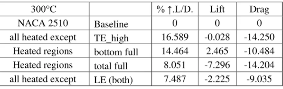
After the trend was confirmed by the second turbulence model, a higher temperature

setting of 300°C was tried on the more favorable four cases. The data obtained in these cases

is synthesized in Tables 5 and 6.

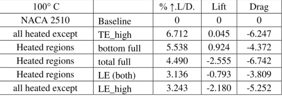
Table 4 – Percent increase in lift and drag depending on heated regions (SST-RC), 100°C

100° C % ↑.L/D. Lift Drag

all heated except TE_high 6.712 0.045 -6.247 Heated regions bottom full 5.538 0.924 -4.372 Heated regions total full 4.490 -2.555 -6.742 Heated regions LE (both) 3.136 -0.793 -3.809 all heated except LE_high 3.243 -2.180 -5.252

Table 5 – Synthesis of Lift and Drag results obtained with the 2D SST-RC model, 300°C

300°C CL/CL_basel. Cd/Cd_basel L/D

(5)

Table 6 – Percent increase in lift and drag depending on heated regions (SST-RC), 300°C

300°C % ↑.L/D. Lift Drag

all heated except TE_high 16.589 -0.028 -14.250 Heated regions bottom full 14.464 2.465 -10.484 Heated regions total full 8.051 -7.296 -14.204 all heated except LE (both) 7.487 -2.225 -9.035

2.2 The narrow tests - 3D CFD

A logical continuation of the study is the 3D narrow wing. Figure 1 depicts the computational domain near the airfoil (the rest of the domain is identical in span as the one used for the 2D cases). In these cases, a steady state RANS using the SST-RC model was used, having an additional set of equations for transition from laminar to turbulent and the Kato-Launder production limiter. The side walls delimiting the airfoil have a periodicity boundary condition.

Fig. 2 – The blocking structure and part details in ICEM CFD meshing software for the 3D narrow test

For the heated cases, the case where all patches were heated with the exception of the

top side of the trailing edge (TE_high). The wall temperature considered was 300°C.

Table 7 presents the aerodynamic coefficients for the heated (Table 7a) and adiabatic (Table 7b) cases.

Table 7 – Aerodynamic coefficients of the airfoils with angle of attack

a) 300°C AoA CL Cd L/d

0 0.255793 0.004812 53.15627 3 0.597122 0.006458 92.46237 5 0.760208 0.009676 78.56526

b) adiabatic AoA CL Cd L/D

(6)

2.3 The 700 mm wide - 3D CFD

Due to the positive results of the narrow 3D case, a wider 3D study was also performed, having a width of 700 mm. The same heated methodology was used as in the previous

section, with the addition of a high temperature test of 300°C. Figure 3 presents the distribution of y+ along the walls of the 300°C heated airfoil.

In these cases, a more detailed analysis with the Detached Eddy Simulation method was used, having the SST-RC with production limiter as a sub-grid-scale model. The time step was chosen in relation with the smallest cell size and the highest local velocity found in the previous simulations. Therefore the time step was fixed at 10-5 seconds, and the physical flow time was sufficient for the fluid to cross the entire length of the domain (5m across). Also, the number of iterations per time step was chosen so that the residual magnitude would drop by at least one order of magnitude.

Fig. 3 – Distribution of y+ value for a 3D 700 mm wide case

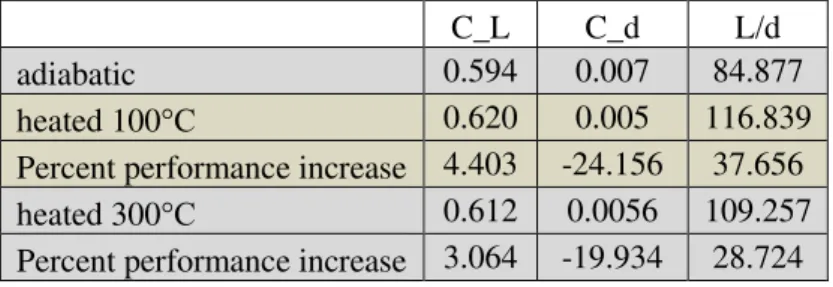
Table 8 – The aerodynamic coefficients of the adiabatic and heated wall airfoil cases

C_L C_d L/d adiabatic 0.594 0.007 84.877 heated 100°C 0.620 0.005 116.839 Percent performance increase 4.403 -24.156 37.656 heated 300°C 0.612 0.0056 109.257 Percent performance increase 3.064 -19.934 28.724

A quick observation is that, for the wider 3D case, the results of the DES simulation is largely the same as in the case of the narrower RANS simulation (at the same angle of attack). More details can be found by post-processing the aerodynamic parameters across the span of the 350 mm chord of the airfoil.

(7)

is that, with temperature, an increasingly higher turbulent kinetic energy is observed in the transition region on the suction side of the airfoil. From Fig.4 it can also be seen that the pressure varies only slightly with temperature after a certain critical value - suggesting an optimal setting.

Fig. 4 – Static pressure chordwise distribution for the three cases studied

Fig. 5 – Aerodynamic skin friction coefficient along the airfoil chord

Perhaps one of the most significant differences noticed in this comparative case study is the aerodynamic friction coefficient. Although the wall was considered to have no surface roughness (due to the negative influence that a wall function modeling would have on the turbulence model), there boundary layer development implies shear stresses on the walls and leads to aerodynamic skin friction.

Figure 5 presents the three studied cases and reveals that the highest friction coefficient appears to be significantly diminished in the heated cases, even though the regions affected are not heated themselves. Also surprising is that this behavior does not appear to influence

(8)

the transition of the boundary layer from laminar to turbulent - which occurs at roughly the same location. Less noticeable from Fig. 5 is that the friction coefficient actually increases slightly near the leading edge of the heated airfoil. In an optimal configuration for heated airfoil, these factors should be considered when determining the heated geometry.

Fig. 6 – First cell temperature for the three cases studied

Figure 6 shows the temperature variation along the blade for the fluid cell nearest to the wall. Again, the region which is not heated - and is considered to be adiabatic - on the top side near the trailing edge appears to be more influenced. The rapid decrease in temperature is mostly due to the heat exchange with the adjacent fluid cells in the higher zones of the boundary layer (since no heat exchange has been considered with the non-heated wall and no radiation model was used). The transition to turbulent is obvious in the 0.1-0.2 m region, as indicated by all other plots presented.

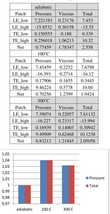
After the general trend lines have been analyzed and some immediate conclusions drawn, we can move to the detailing of the viscous and pressure forces acting on the four patches of the airfoil and compare the baseline adiabatic case with the two heated cases. The parameters are presented in Table 9 for the drag forces and in Table 10 for the lift forces.

Fig. 7 – Drag force breakdown, relative to the adiabatic baseline 0,5

0,6 0,7 0,8 0,9 1 1,1

adiabatic 100 C 300 C

Pressure

Viscous

(9)

Table 9 – Breakdown of drag forces

adiabatic

Patch Pressure Viscous Total LE_low 7.221193 0.23176 7.453 LE_high -15.8532 0.30158 -15.55

TE_low 0.150555 0.188 0.339 TE_high 9.256018 1.06213 10.32 Net 0.77459 1.78347 2.558

100°C

Patch Pressure Viscous Total LE_low 7.45459 0.2252 7.6798 LE_high -16.393 0.2714 -16.12 TE_low 0.17906 0.1655 0.3445 TE_high 9.46224 0.5778 10.04

Net 0.70256 1.2399 1.9424 300°C

Patch Pressure Viscous Total LE_low 7.39074 0.22057 7.61132 LE_high -16.227 0.23317 -15.994 TE_low 0.16939 0.14003 0.30942 TE_high 9.49909 0.62468 10.1238 Net 0.83212 1.21845 2.05058

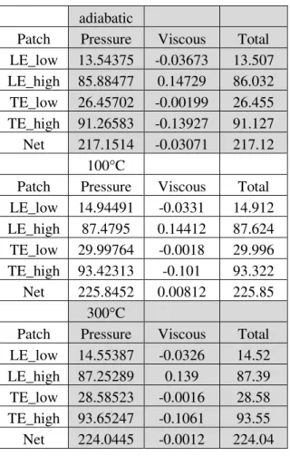
Fig. 8 – Lift force breakdown, relative to the adiabatic baseline (viscous lift is negligible)

A simple examination of Figs.7 and 8 reveals that in the case where high temperature was used, the pressure distribution along the airfoil surface leads to higher pressure drag as well as a slightly lower increase in pressure lift. This can be associated with the slight shift in the stagnation point near the leading edge, but the interaction with the flow is more complex than this. Also, although most of the drag is viscous, the pressure drag may also be reduced through careful distribution of heated patches on the airfoil surface. In addition to the

0,97 0,98 0,99 1 1,01 1,02 1,03 1,04 1,05

adiabatic 100 C 300 C

Pressure

(10)

geometrical position of the heated patches, it becomes apparent that the value of the temperature - in this case study - and the distribution of heat exchange - in the broader principle - is relevant to the influence on pressure drag and lift.

This conclusion is very important for the next stages of the heated airfoil where higher cambered airfoils will be tested. In these, pressure - rather than viscous - forces dominate drag as well as lift.

Table 10 – Breakdown of lift forces

adiabatic

Patch Pressure Viscous Total LE_low 13.54375 -0.03673 13.507 LE_high 85.88477 0.14729 86.032 TE_low 26.45702 -0.00199 26.455 TE_high 91.26583 -0.13927 91.127 Net 217.1514 -0.03071 217.12

100°C

Patch Pressure Viscous Total LE_low 14.94491 -0.0331 14.912 LE_high 87.4795 0.14412 87.624 TE_low 29.99764 -0.0018 29.996 TE_high 93.42313 -0.101 93.322 Net 225.8452 0.00812 225.85

300°C

Patch Pressure Viscous Total LE_low 14.55387 -0.0326 14.52 LE_high 87.25289 0.139 87.39 TE_low 28.58523 -0.0016 28.58 TE_high 93.65247 -0.1061 93.55 Net 224.0445 -0.0012 224.04

3. CONCLUSIONS

A CFD case study was conducted, comparing the aerodynamic performances of a simple NACA airfoil with low camber curvature with adiabatic walls and with heated patches. The chord of the airfoil was 0.35 m and the ambient velocity 50 m/s with the temperature of the heated patches of either 100 °C and 300°C

Preliminary 2D CFD studies were performed using two turbulence models which do not use wall functions. Various combinations of heated/adiabatic patches were tested with both models. The most promising setting was chosen for a narrow 3D case with periodicity. During this second test round, the angle of attack was varied, indicating that the lower incidences lead to more beneficial effects on the lift to drag ratio.

(11)

Detached Eddy Simulation model was used, having the SST-RC with Kato-Launder turbulence production as a sub-grid scale model.

Surprisingly, the 2D simulations under predict the influence of the heated walls on the aerodynamic behavior of the airfoil.

Findings show that the optimal setup for the heated airfoil should include all areas, with the exception of the top side near the trailing edge.

Also, temperature seems to have a moderate effect on the overall lift and drag. This is however not a simple consequence of temperature, but rather an interactive effect that the temperature distribution has in a given context. It is therefore to be expected that different airfoils at different angles of attack and Reynolds numbers will have different optimal temperature values as well as distribution.

Static pressure appears to increase due to boundary layer heating, but the overall pressure increase around the airfoil depends on the local velocity magnitude outside the boundary layer.

While heating does not have an impact on the location of the transition from laminar to turbulent flow, it does cause the turbulent kinetic energy to be higher in the heated cases.

Another aspect refers to the decrease of the Reynolds number near the wall, which is mainly due to the increase in local viscosity with temperature. The positive influence can be seen in the wall shear stress and skin friction coefficient.

Therefore, overall viscous drag is reduced with temperature but not in a linear relation. However, pressure lift and drag depend on the way temperature is distributed across the airfoil.

Further work should include a theoretical development of the optimal method to carry out this type of flow control, aiming for an application of a highly cambered airfoil.

Also, an interesting avenue to be explored is the interaction with other high-lift devices such as leading edge or trailing edge flaps, Gurney type devices or vortex generators such as chevrons and tabs.

REFERENCES

[1] T. Nonweiler, H. Y. Wong, S. R. Aggarwal, The Role of Heat Conduction in Leading Edge Heating Theory and Experiment, University of Glasgow Dept. of Aeronautics and Fluid Mechanics, C.P. No. 1126,1970. [2] Z. X. Yuan, W. Q. Tao, X. T. Yan, Experimental Study on Heat Transfer in Ducts with Winglet Disturbances,

Heat Transfer Engineering, 24(2):1–9, ISSN0145-7632 (Print), 1521-0537 (Online) 2003, Copyright C 2003 Taylor & Francis.

[3] F. J. Edwards and C. J. R. Alker, The Improvement of Forced Convection Surface Heat Transfer Using Surface Protrusions in the Form of (A) Cubes and (B) Vortex Generators, Fifth International Heat Transfer Conference, Tokyo, Vol. 2, pp. 244-248, 1974.

[4] F. Xie, Z.Y. Ye, The simulation of the airship flow field with injection channel for the drag reduction, Eng. Mech.27 (2), 2010.

[5] J. Hua, F. Kong, H. H. T. Liu, Unsteady Thermodynamic CFD Simulations of Aircraft Wing Anti-Icing Operation, Journal of Aircraft, Vol. 44, No. 4, pp. 1113-1117, ISSN: 0021-8669, EISSN: 1533-3868,July

– August 2007.

[6] R. Kamboj, S. Dhingra, G. Singh, CFD Simulation of Heat Transfer Enhancement by Plain and Curved Winglet Type Vertex Generators with Punched Holes, International Journal of Engineering Research and General Science, ISSN 2091-2730, Volume 2, Issue 4, pp. 648 – 659, June-July, 2014.

[7] H. H. T. Liu and J. Hua, Three-Dimensional Integrated Thermodynamic Simulation for Wing Anti-Icing System, Journal of Aircraft, Vol. 41, No. 6, pp 1291-1297, ISSN: 0021-8669, EISSN: 1533-3868, 2004. [8] T. F. Gelder and J. P. Lewis, Comparison of Heat Transfer from Airfoil in Natural and Simulated Icing

Conditions, Lewis Flight Propulsion Laboratory Cleveland, NACA Technical Note 2480, Ohio 1951. [9] C. W. Frick, Jr. and G. B. McCullough, Tests of Heated Low-Drag Airfoil, NACA ACR, Ames Aeronautical

(12)

[10] P. Spalart and S. Allmaras, A one-equation turbulence model for aerodynamic flows, Technical Report AIAA-92-0439, American Institute of Aeronautics and Astronautics, 1992.

[11] F. R. Menter, Two-Equation Eddy-Viscosity Turbulence Models for Engineering Applications, AIAA Journal, 32(8):1598-1605, ISSN: 0001-1452, EISSN: 1533-385X, August 1994.

[12] P. R. Spalart and M. L. Shur, On the Sensitization of Turbulence Models to Rotation and Curvature, Aerospace Sci. Tech., 1(5). 297–302, doi:10.1016/S1270-9638(97)90051-1, 1997.

[13] M. L. Shur, M. K. Strelets, A. K. Travin and P. R. Spalart, Turbulence Modeling in Rotating and Curved Channels: Assessing the Spalart-Shur Correction, AIAA Journal, 38(5), pp. 784-792, May 2000.

[14] R. H. Nichols, Turbulence Models and Their Application to Complex Flows, University of Alabama at Birmingham, Revision 4.01, 2014.

[15] T. T. Rodrigues, R. Link, Effect of the Turbulence Modeling in the Prediction of Heat Transfer in Suction Mufflers, International Compressor Engineering Conference, July 16-19, 2012.