S. Fr¨oschle, F.D. Valencia (Eds.): Workshop on Expressiveness in Concurrency 2010 (EXPRESS’10). EPTCS 41, 2010, pp. 91–105, doi:10.4204/EPTCS.41.7
This work is licensed under the Creative Commons Attribution License. Gavin Lowe
We consider models of CSP based on recording what events are available as possible alternatives to the events that are actually performed. We present many different varieties of such models. For each, we give a compositional semantics, congruent to the operational semantics, and prove full abstraction and no-junk results. We compare the expressiveness of the different models.
1
Introduction
In this paper we consider a family of semantic models of CSP [13] that record what events a process makes available as possible alternatives to the events that are actually performed. For example, the models will distinguish a→STOP✷b→STOPand a→STOP⊓b→STOP: the former offers its environment the choice betweena and b, so can makea available before performing b; however the latter decides internally whether to offeraorb, so cannot makeaavailable before performingb.
A common way of motivating process algebras (dating back to [8]) is to view a process as a black box with which the observer interacts. The models in this paper correspond to that black box having a light for each event that turns on when the event is available (as in [5, 4]); the observer can record which lights turn on in addition to which events are performed.
I initially became interested in such models by considering message-passing concurrent program-ming languages that allow code to test whether a channel is ready for communication without actu-ally performing the communication. In [7], I considered the effect of extending CSP with a construct “if readyathenPelseQ” that tests whether the eventais ready for communication (i.e., whether this pro-cess’s environment is ready to performa), acting likePorQappropriately. The model in [7] recorded what events were made available by a process, in addition to the events actually performed. We investi-gate such models more fully in this paper. We show that —even without the above construct— there are many different variations, with different expressive power.
By convention, a denotational semantic model of CSP is alwayscompositional, i.e., the semantics of a composite process is given in terms of the semantics of its components. Further, there are several other desirable properties of semantic models:
Congruence to the operational semantics The denotational semantics can either be extracted from the operational semantics, or calculated compositionally, both approaches giving the same result;
Full abstraction The notion of semantic equivalence corresponds to some natural equivalence, typically defined in terms of testing;
No-junk The denotational semantic domain corresponds precisely to the semantics of processes: for
each element of the semantic domain, we can construct a corresponding process.
Each of the semantic models in this paper satisfies these properties.
In Section 3 we describe variations on the basic model, in two dimensions: one dimension restricts the number of observations of availability between successive standard events; the other dimension allows the simultaneous availability of multiple events to be recorded. For each resulting model, we describe compositional semantics, and full abstraction and no-junk results (we omit some of the details because of lack of space, and to avoid repetition). We then study the relative expressive power of the models.
Finally, in Section 4, we discuss various aspects of our models, some additional potential models, and some related work.
Overview of CSP We give here a brief overview of the syntax and semantics of CSP; for simplicity and brevity, we consider a fragment of the language in this paper. We also give a brief overview of the Traces and Stable Failures Models of CSP. For more details, see [6, 13].
CSP is a process algebra for describing programs orprocesses that interact with their environment by communication. Processes communicate via atomic events, from some setΣ. Events often involve passing values over channels; for example, the eventc.3 represents the value 3 being passed on channelc. The simplest process isSTOP, which represents a deadlocked process that cannot communicate with its environment. The processdivrepresents a divergent process that can only perform internal events.
The processa→Poffers its environment the eventa; if the event is performed, it then acts likeP. The processc?x→Pis initially willing to input a valuexon channelc, i.e. it is willing to perform any event of the formc.x; it then acts likeP(which may usex). Similarly, the process ?a:A→Pis initially willing to perform any eventafromA; it then acts likeP(which may usea).
The process P✷Qcan act like eitherP orQ, the choice being made by the environment: the en-vironment is offered the choice between the initial events ofPand Q. By contrast,P⊓Qmay act like eitherPorQ, with the choice being made internally, not under the control of the environment;
⊓
x:XPx nondeterministically acts like anyPxforxinX. The processP⊲Qrepresents a sliding choice or timeout: it initially acts likeP, but if no event is performed then it can internally change state to act likeQ.The process PAkB Q runs Pand Qin parallel; P is restricted to performing events from A; Qis restricted to performing events fromB; the two processes synchronise on events fromA∩B. The process P|||QinterleavesPandQ, i.e. runs them in parallel with no synchronisation.
The processP\Aacts likeP, except the events fromAare hidden, i.e. turned into internal, invisible events, denotedτ, which do not need to synchronise with the environment. The processP[[R]]represents Pwhere events are renamed according to the relationR, i.e.,P[[R]]can perform an eventbwheneverP can perform an eventasuch thata R b.
Recursive processes may be defined equationally, or using the notation µX•P, which represents a process that acts likeP, where each occurrence ofXrepresents a recursive instantiation ofµX•P.
Prefixing (→) binds tighter than each of the binary choice operators, which in turn bind tighter than the parallel operators.
CSP can be given both an operational and denotational semantics. The denotational semantics can either be extracted from the operational semantics, or defined directly over the syntax of the language; see [13]. It is more common to use the denotational semantics when specifying or describing the be-haviours of processes, although most tools act on the operational semantics. Atraceof a process is a sequence of (visible) events that a process can perform. Iftris a trace, thentr↾Arepresents the restric-tion oftrto the events inA, whereastr\Arepresentstrwith the events fromAremoved; concatenation is written “⌢”;A∗represents the set of traces with events fromA. Astable failureof a process Pis a
2
Availability information
In this section we consider a model that record that particular events are available during an execution. We begin by extending the operational semantics so as to formally define this notion of availability. We then define our semantic domain —traces containing both standard events and availability information— with suitable healthiness conditions. We then present compositional trace semantics, and show that it is congruent to the operational semantics. Finally, we prove full abstraction and no-junk results.
We write offer ato record that the eventais offered by a process, i.e. ais available. We augment the operational semantics with actions to record such offers (we term theseactions, to distinguish them from standard events). Formally, we define a new transition relation −−⊲from the standard transition relation−→(see [13, Chapter 7]) by:
P−−α⊲Q ⇔ P−→α Q, forα∈Σ∪ {τ}, Poffer a−−⊲P ⇔ P−→a .
For example: a→STOP✷b→STOP offer a−−⊲ a→STOP✷b→STOP −−b⊲ STOP.Note that the transi-tions corresponding toofferactions do not change the state of the process.
We now consider an appropriate form for the denotational semantics. One might wonder whether it is enough to record availability information only at theend of a trace (by analogy to the stable failures model). However, a bit of thought shows that such a model would be equivalent to the standard Traces Model: a process can perform the tracetr⌢hoffer aiprecisely if it can perform the standard tracetr⌢hai. We therefore record availability information throughout the trace. For convenience, for A⊆Σ, we define
offer A={offer a|a∈A}, A†=A∪offer A, A†τ =A†∪ {τ}.
We define anavailability trace to be a sequence trin(Σ†)∗. We can extract the traces (of Σ† actions)
from the operational semantics (following the approach in [13, Chapter 7]):
Definition 1 We writeP7−→s Q, fors=hα1, . . . ,αni ∈(Σ†τ)∗, if there existP0=P,P1, . . . ,Pn=Qsuch thatPi
αi+1
−−⊲Pi+1fori=0, . . . ,n−1. We writeP
tr
=⇒Q, fortr∈(Σ†)∗, if there is somessuch thatP s
7−→Q andtr=s\τ.
Example 2 The process a→STOP✷b→STOPhas the availability trace hoffer a,bi. However, the
processa→STOP⊓b→STOPdoes not have this trace. This model therefore distinguishes these two processes, unlike the standard Traces Model.
Note in particular that we may record the availability of events in unstable states (whereτ events are available), by contrast with models like the Stable Failures Model that record (un)availability information only in stable states. The following example contrasts the two models.
Example 3 The processesa→STOPand a→STOP⊓STOPare distinguished in the Stable Failures
Model, since the latter has stable failure(hi,{a}); however they have the same availability traces. The processes(a→STOP⊲b→STOP)⊓(b→STOP⊲a→STOP)anda→STOP⊓b→STOPare distinguished in the Availability Traces Model, since only the former has the availability tracehoffer a,bi; however, they have the same stable failures.
The availability-traces of process P are then {tr|P=tr⇒}. The following definition captures the properties of this model.
Definition 4 TheAvailability Traces ModelA contains those setsT ⊆(Σ†)∗that satisfy the following
1. Tis non-empty and prefix-closed.
2. offeractions can always be remove from or duplicated within a trace:
tr⌢hoffer ai⌢tr′∈T ⇒ tr⌢hoffer a,offer ai⌢tr′∈T∧tr⌢tr′∈T
.
3. If a process can offer an event it can perform it: tr⌢hoffer ai ∈T ⇒ tr⌢hai ∈T.
4. If a process can perform an event it can first offer it: tr⌢hai⌢tr′∈T ⇒ tr⌢hoffer a,ai⌢tr′∈T.
Lemma 5 For all processesP, {tr|P=tr⇒}is an element of the Availability Traces Model, i.e., satisfies the four healthiness conditions.
Compositional traces semantics We now give compositional rules for the traces of a process. We write tracesA[[P]]for the traces ofP1. Below we will show that these are congruent to the operational definition above.
STOPanddivare equivalent in this model: they can neither perform nor offer standard events. The processa→Pcan initially signal that it is offeringa; it can then performa, and continue likeP.
tracesA[[STOP]] = tracesA[[div]] = {hi}
tracesA[[a→P]] = {offer a}∗∪ {tr⌢hai⌢tr′|tr∈ {offer a}∗∧tr′∈tracesA[[P]]}.
The process P⊲Q can either perform a trace of P, or can perform a trace of P with no standard events, and then (after the timeout) perform a trace ofQ. The processP⊓Qcan perform traces of either of its components; the semantics of replicated nondeterministic choice is the obvious generalisation.
tracesA[[P⊲Q]] = tracesA[[P]]∪ {trP⌢trQ|trP∈tracesA[[P]]∧trP↾Σ=hi ∧trQ∈tracesA[[Q]]},
tracesA[[P⊓Q]] = tracesA[[P]]∪tracesA[[Q]],
tracesA[[
⊓
i∈IPi]] = [i∈ItracesA[[Pi]].
Before the first visible event, the processP✷Qcan perform anoffer aaction ifeither PorQcan do so. Lettr|||tr′be the set of ways of interleavingtrandtr′(this operator is defined in [13, page 67]). The three sets in the definition below correspond to the cases where (a) neither process performs any visible events, (b)Pperforms at least one visible event (after which,Qis turned off), and (c) the symmetric case whereQperforms at least one visible event.
tracesA[[P✷Q]] =
{tr| ∃trP∈tracesA[[P]],trQ∈tracesA[[Q]]•trP↾Σ=trQ↾Σ=hi ∧tr∈trP|||trQ} ∪
{tr⌢hai⌢tr′
P| ∃trP⌢hai⌢tr′P∈tracesA[[P]],trQ∈tracesA[[Q]]• trP↾Σ=trQ↾Σ=hi ∧a∈Σ∧tr∈trP|||trQ} ∪
{tr⌢hai⌢tr′
Q| ∃trP∈tracesA[[P]],trQ⌢hai⌢trQ′ ∈tracesA[[Q]]• trP↾Σ=trQ↾Σ=hi ∧a∈Σ∧tr∈trP|||trQ}.
In a parallel composition of the formPAkBQ, Pis restricted to actions fromA†, andQis restricted to actions fromB†. Further,PandQmust synchronise upon both standard events fromA∩Band offers of events fromA∩B. We writetrP k
(A∩B)†
trQfor the set of ways of synchronisingtrP andtrQon actions
1We include the subscript “A” intraces
from(A∩B)†(this operator is defined analogously to in [13, page 70]). The semantics of interleaving is
similar.
tracesA[[PAkBQ]] = {tr| ∃trP∈tracesA[[P]]∩(A†)∗,trQ∈tracesA[[Q]]∩(B†)∗ •tr∈trP k (A∩B)†
trQ}.
tracesA[[P|||Q]] = {tr| ∃trP∈tracesA[[P]],trQ∈tracesA[[Q]]•tr∈trP|||trQ}.
The semantic equation for hiding ofAcaptures thatoffer Aactions are blocked, andAevents are in-ternalised. For relational renaming, we lift the renaming to apply tooffer actions, i.e.(offer a)R(offer b) if and only ifa R b; we then lift the relation to traces by pointwise application. The semantic equation is then a further lift ofR.
tracesA[[P\A]] = {trP\A|trP∈tracesA[[P]]∧trP↾offer A=hi}.
tracesA[[P[[R]]]] = {tr| ∃trP∈tracesA[[P]]•trPR tr}.
We now consider the semantics of recursion. Our approach follows the standard method using com-plete partial orders; see, for example, [13, Appendix A.1].
Lemma 6 The Availability Traces Model forms a complete partial order under the subset ordering⊆,
withtracesA[[div]]as the bottom element.
Lemma 7 Each of the operators is continuous with respect to the⊆ordering.
Hence from Tarski’s Theorem, each mappingFdefinable using the operators of the language has a least fixed point given bySn>0Fn(div). This justifies the following definition.
tracesA[[µX•F(X)]] =the⊆-least fixed point of the semantic mapping corresponding toF.
The following theorem shows that the two ways of capturing the traces are congruent; it can be proved by a straightforward structural induction.
Theorem 8 For all tracestr∈(Σ†)∗: tr∈traces
A[[P]]iffP tr =⇒.
Theorem 9 For all processes,tracesA[[P]]is a member of the Availability Traces Model (i.e., it satisfies the conditions of Definition 4).
Full abstraction We can show that this model is fully abstract with respect to a form of testing in the style of [10]. We consider tests that may detect the availability of events. Following [7], we write readya&T for a test that tests whetherais available, and if so acts like the testT. We also allow a test SUCCESSthat represents a successful test, and a simple form of prefixing. Formally, tests are defined by the grammar:
T ::= SUCCESS|a→T|readya&T.
We consider testing systems comprising a testTand a processP, denotedTkP. We define the seman-tics of testing systems by the rules below; ω indicates that the test has succeeded, and Ωrepresents a terminated testing system.
SUCCESSkP −→ω Ω P
τ
−−⊲ Q
P −−a⊲ Q
a→TkP −→τ TkQ
P offer a−−⊲ P
readya&TkP −→τ TkP
We say thatPmay pass the testT, denotedPmayT, ifTkPcan performω (after zero or moreτs). We now show that if two processes are denotationally different, we can produce a test to distinguish them, i.e., such that one process passes the test, and the other fails it. Lettr∈(Σ†)∗. We can construct a
testTtrthat detects the tracetr.
Thi = SUCCESS,
Thai⌢tr = a→Ttr,
Thoffer ai⌢tr = readya&Ttr.
The following lemma can be proved by a straightforward induction on the length oftr:
Lemma 10 For all processesP, PmayTtr if and only iftr∈tracesA[[P]].
Theorem 11 tracesA[[P]] =tracesA[[Q]]if and only ifPandQpass the same tests.
Proof:The only if direction is trivial. IftracesA[[P]]6=tracesA[[Q]]then without loss of generality suppose tr∈tracesA[[P]]−tracesA[[Q]]; thenPmayTtrbut notQmayTtr. ✷
We now show that the model contains no junk: each element of the model corresponds to a process.
Theorem 12 LetT be a member of the Availability Traces Model. Then there is a processPsuch that
tracesA[[P]] =T.
Proof:Lettrbe a trace. We can construct a processPtras follows:
Phi = STOP,
Phai⌢tr = a→Ptr, Phoffer ai⌢tr = a→div⊲Ptr.
Then the traces ofPtrare justtrand those traces implied fromtrby the healthiness conditions of Defini-tion 4. Formally, we can prove this by inducDefini-tion ontr. For example:
• The traces ofPhai⌢tr are prefixes of traces of the form2 (offer a)k⌢hai⌢tr′, wherek>0 and tr′ is a trace of Ptr. Hence (by the inductive hypothesis) tr′ is implied from tr by the healthiness conditions. Thushai⌢tr′is implied fromhai⌢tr. Finally(offer a)k⌢hai⌢tr′is implied fromhai⌢tr bykapplications of healthiness condition 4.
• The traces ofPhoffer ai⌢trare of two forms:
– Prefixes of traces of the form (offer a)k⌢hai, which is implied fromhoffer ai by healthiness conditions 2 and 3.
– Traces of the form(offer a)k⌢tr′ wheretr′ is a trace ofP
tr. Hence (by the inductive hypoth-esis) tr′ is implied from tr by the healthiness conditions. And so (offer a)k⌢tr′ is implied
fromhoffer ai⌢trby healthiness condition 2.
ThenP=
⊓
tr∈TPtris such thattracesA[[P]] =T. ✷3
Variations
In this section we consider variations on the model of the previous section, extending the models along essentially two different dimensions. We first consider models that place a limit on the number ofoffer actions between consecutive standard events. We then consider models that record the availability of setsof events. Finally we combine these two variations, to produce a hierarchy of different models with different expressive power (illustrated in Figure 1). For each variant, we sketch how to adapt the semantic model and full abstraction result from Section 2. We concentrate on discussing the relationship between the different models.
3.1 Bounded availability actions
Up to now, we have allowed arbitrarily manyofferactions between consecutive standard events. It turns out that we can restrict this. For example, we could allow at most oneofferaction between consecutive standard events (or before the first event, or after the last event). This model is more abstract than the previous; for example, it identifies the processes
(a→STOP✷b→STOP)⊓(a→STOP✷c→STOP)⊓(b→STOP✷c→STOP)
and
(a→STOP✷b→STOP✷c→STOP),
whereas the previous model distinguished them by the tracehoffer a,offer b,ci.
More generally, we define the model that allows at most n offer actions between consecutive standard events. Let Obsn be the set of availability traces with this property. Then the model An is the restriction of A to Obsn, i.e., writing tracesA,n for the semantic function for An, we have tracesA,n[[P]] =tracesA[[P]]∩Obsn. In particular,A0is equivalent to the standard traces model.
The following example shows that the models become strictly more refined asnincreases; further, the full Availability Traces ModelA is finer than each of the approximationsAn.
Example 13 Consider the processes
P0 = STOP
Pn+1 = (a→STOP⊓b→STOP)⊲Pn.
Suppose n is non-zero and even (the case of odd n is similar). Processes Pn and Pn+1 can be
dis-tinguished in model An and model A, since only Pn+1 has the trace hoffer a,offer b,offer a,offer b, . . . ,offer a,offer b,aiwithn offeractions. However, these processes are equal in modelAn−1.
Following Roscoe [15], we writeMM′if modelM′is finer (i.e. distinguishes more processes) than modelM, and≺for the corresponding strict relation. The above example shows
A0≡T ≺A1≺A2≺. . .≺A.
In some cases, the semantic equations have to be adapted slightly to ensure the traces produced are indeed fromObsn, for example:
tracesA,n[[PAkBQ]] =
{tr| ∃trP∈tracesA,n[[P]]∩(A†)∗,trQ∈tracesA,n[[Q]]∩(B†)∗ •tr∈(trP k (A∩B)†
trQ)∩Obsn}.
The healthiness conditions need to be adapted slightly to reflect that only traces from Obsn are in-cluded. For example, condition 4 becomes
4′. tr⌢hai⌢tr′∈T∧tr⌢hoffer a,ai⌢tr′∈Obs
n⇒tr⌢hoffer a,ai⌢tr′∈T.
Finally, the full abstraction result still holds, but the tests need to be restricted to include at mostn successivereadytests. And the no-junk result still holds.
3.2 Availability sets
The models we have considered so far have considered the availability of asingleevent at a time. If we consider the availability of aset of events, can we distinguish more processes? The answer turns out to be yes, but only with processes that can either diverge or that exhibit unbounded nondeterminism (a result which was surprising to me).
We will consider actions of the formoffer A, whereAis a set of events, representing that all the events inAare simultaneously available. We can adapt the derived operational semantics appropriately:
P−−α⊲PQ ⇔ P
α
−→Q, forα ∈Σ∪ {τ},
Poffer A−−⊲PP ⇔ ∀a∈A•P
a
−→.
For convenience, we define
AP† = A∪ {offer B|B∈PA}
.
Traces will then be from(ΣP†)∗. We can extract traces of this form from the derived operational semantics
as in Definition 1 (writing7−→tr Pand
tr
=⇒Pfor the corresponding relations).
We call this model the Availability Sets Traces Model, and will sometimes refer to the previous model as the Singleton Availability Traces Model, in order to emphasise the difference.
Definition 14 The Availability Sets Traces ModelAP contains those sets T⊆(ΣP†)∗ that satisfy the
following conditions.
1. Tis non-empty and prefix-closed.
2. offeractions can always be removed from or duplicated within a trace:
tr⌢hoffer Ai⌢tr′∈T ⇒ tr⌢hoffer A,offer Ai⌢tr′∈T∧tr⌢tr′∈T .
3. If a process can offer an event it can perform it: tr⌢hoffer Ai ∈T ⇒ ∀a∈A•tr⌢hai ∈T. 4. If a process can perform an event it can first offer it:
tr⌢hai⌢tr′∈T ⇒ tr⌢hoffer{a},ai⌢tr′∈T.
5. The offers of a process are subset-closed
tr⌢hoffer Ai⌢tr′∈T∧B⊆A ⇒ tr⌢hoffer Bi⌢tr′∈T.
Lemma 15 For all processesP, {tr|P=tr⇒P}is an element of the Availability Sets Traces Model.
Compositional semantics We give below semantic equations for the Availability Sets Traces Model.
Most of the clauses are straightforward adaptations of the corresponding clauses in the Singleton Avail-ability Traces Model.
For the parallel operators and external choice, we define an operator k
X
P
such thattrk
X
P
tr′ gives all
traces resulting from tracestrandtr′, synchronising on events and offers of events fromX. The definition is omitted due to space restrictions.
For relational renaming, we lift the renaming to apply toofferactions, by forming the subset-closure of the relational image:
(offer A)R(offer B) ⇔ ∀b∈B•∃a∈A•a R b.
We again lift it to traces pointwise. The semantic clauses are as follows.
tracesPA[[STOP]] =tracesAP[[div]] = (offer{})∗,
tracesP
A[[a→P]] =Init∪ {tr
⌢hai⌢tr′|tr∈Init∧tr′∈tracesP
A[[P]]}, whereInit={offer{},offer{a}}∗,
tracesP
A[[P⊲Q]] =traces
P
A[[P]]∪ {trP⌢trQ|trP∈tracesPA[[P]]∧trP↾Σ=hi ∧trQ∈tracesPA[[Q]]}, tracesPA[[P⊓Q]] =tracesPA[[P]]∪tracesPA[[Q]],
tracesP
A[[P✷Q]] =
{tr| ∃trP∈tracesPA[[P]],trQ∈tracesPA[[Q]]•trP↾Σ=trQ↾Σ=hi ∧tr∈trP k
{}
P
trQ} ∪
{tr⌢hai⌢tr′
P| ∃trP⌢hai⌢tr′P∈traces
P
A[[P]],trQ∈traces
P
A[[Q]]• trP↾Σ=trQ↾Σ=hi ∧a∈Σ∧tr∈trP k
{}
P
trQ} ∪
{tr⌢hai⌢tr′
Q| ∃trP∈traces
P
A[[P]],trQ⌢hai⌢tr′Q∈traces
P
A[[Q]]• trP↾Σ=trQ↾Σ=hi ∧a∈Σ∧tr∈trP k
{}
P
trQ},
tracesPA[[PAkBQ]] ={tr| ∃trP∈tracesPA[[P]]∩(AP†)∗,trQ∈tracesPA[[Q]]∩(BP†)∗ •tr∈trP k A∩B
P
trQ},
tracesPA[[P|||Q]] ={tr| ∃trP∈tracesPA[[P]],trQ∈tracesPA[[Q]]•tr∈trP k
{}
P
trQ},
tracesP
A[[P\A]] ={trP\A|trP∈tracesAP[[P]]∧ ∀X•offer XintrP⇒X∩A={}}, tracesPA[[P[[R]]]] ={tr| ∃trP∈tracesPA[[P]]•trPR tr},
tracesPA[[µX•F(X)]] =the⊆-least fixed point of the semantic mapping corresponding toF.
Theorem 16 The semantics is congruent to the operational semantics:tr∈tracesPA[[P]]iffP=tr⇒P.
Full abstraction In order to prove a full abstraction result, we extend our class of tests to include a test of the formreadyA&P, which tests whether all the events inAare available, and if so acts like the testT. Formally, this test is captured by the following rule.
Poffer A−−⊲P
Giventr∈(ΣP†)∗, we can construct a testT
trthat detects the tracetras follows.
Thi = SUCCESS
Thai⌢tr = a→Ttr
Thoffer Ai⌢tr = readyA&Ttr
The full abstraction proof then proceeds precisely as in Section 2.
We can prove a no-junk result as in Section 2. Given trace tr, we can construct a process Ptr as follows:
Phi = STOP,
Phai⌢tr = a→Ptr,
Phoffer Ai⌢tr = (?a:A→div)⊲Ptr.
Then the traces of Ptr are just tr and those traces implied from tr by the healthiness conditions. Again, given an elementT from the Availability Sets Traces Model, we can defineP=
⊓
tr∈TPtr; then tracesP
A[[P]] =T.
Distinguishing power We now consider the extent to which the Availability Sets Model can distinguish processes that the Singleton Availability Model can’t.
Example 17 The Availability Sets Traces Model distinguishes the processes
P = a→STOP✷b→STOP,
Q = (a→STOP⊓b→STOP)⊲Q,
since justPhas the tracehoffer{a,b}i. However, these are equivalent in the Singleton Availability Traces Model; in particular, both can perform arbitrary sequences ofoffer aandoffer bactions initially.
The processQabove can diverge (i.e., perform an infinite number of internalτ events corresponding to timeouts). We can obtain a similar effect without divergence, but using unbounded nondeterminism.
Example 18 Consider
Q0 = STOP,
Qn+1 = (a→STOP⊓b→STOP)⊲Qn, Q′ =
⊓
n∈NQn.
ThenP(from the previous example) andQ′are distinguished in the Availability Sets Traces Model but not the Singleton Availability Traces Model.
For finitely nondeterministic, non-divergent processes, it is enough to consider the availability of onlyfinitesets, since such a process can offer an infinite setAiff and only if it can offer all its finite sub-sets. However, for infinitely nondeterministic processes, one can make more distinctions by considering infinite sets.
Example 19 LetAbe an infinite set of events. Consider the processes
?a:A→STOP and
⊓
b∈A?a:A− {b} →STOP
Proposition 20 IfPandQare non-divergent, finitely nondeterministic processes, that are equivalent in the Singleton Availability Model, then they are equivalent in the Availability Sets Model.
Proof:Suppose, for a contradiction, thatPandQare non-divergent and finitely deterministic, are equiv-alent in the Singleton Availability Model, but are distinguished in the Availability Set Model. Then, without loss of generality, there are tracestrandtr′, and set of eventsAsuch thattr⌢hoffer Ai⌢tr′ is a trace ofP but not ofQ. By the discussion in the previous paragraph, we may assume, without loss of generality, thatAis finite, sayA={a1, . . . ,an}. SinceQis non-divergent and finitely-nondeterministic, there is some bound, k say, on the number of consecutive τ events that it can perform after tr. Since Pcan offer all ofAaftertr, it can also offer any individual events from A, sequentially, in an arbitrary order. In particular, it has the singleton availability trace
tr⌢hoffer a
1, . . . ,offer anik+1⌢tr′.
SincePandQare, by assumption, equivalent in the Singleton Availability model,Qalso has this trace. Qmust perform at mostkτ events within the sub-tracehoffer a1, . . . ,offer anik+1. This tells us that there is a sub-trace within that, of lengthn, containing no τ events. Within this sub-trace there are no state changes (i.e., there are only self-loops corresponding to theofferactions), and so all theai are offered in the same state. Hencetr⌢hoffer Ai⌢tr′is an availability set trace ofQ, giving a contradiction. ✷
Bounded sets We can consider some variants on the Availability Sets Traces Model.
First, let us consider the modelAkthat places a limit of sizekupon availability sets. It is reasonable straightforward to produce compositional semantics for such models, and to adapt the full abstraction and no-junk results. It is perhaps surprising that such a semantics is compositional, since a similar result does not hold for stable failures [1] (although it is conjectured in [15] that this does hold for acceptances). Clearly,A1≡A, andA0≡T (the standard traces model). Examples 17 and 18 show thatA2is
finer thatA1. We can generalise those examples to show that each modelAkis finer thanAk−1.
Example 21 LetAk be a set of sizek. Consider
Pk = ?a:Ak→STOP,
Qk =
⊓
b∈Ak(?a:Ak− {b} →STOP)⊲Qk.ThenPkandQkare distinguished inAksince onlyPkhas the tracehoffer Aki. However they are equiva-lent inAk−1: in particular, both can initially perform any trace of offers of sizek−1.
The limit of the modelsAk considers arbitraryfiniteavailability sets; we term thisAF. The model AF
distinguishes the processesPkandQkfrom Example 21, for allk, so is finer than each of the models with bounded availability sets. As shown by Example 19,AF
is coarser thanAP
.
In fact, for an arbitrary infinite cardinal κ, we can consider the model Aκ that places a limit of sizeκ upon availability sets. Example 19 showed that considering finite availability sets distinguishes fewer processes than allowing infinite availability sets, i.e.AF
≺Aκ. The following example shows that the models become finer asκincreases.
Example 22 Pick an infinite cardinalκ, and pick alphabetΣsuch thatcard(Σ)>κ. Then the processes
Pκ =
⊓
A⊆Σ,card(A)=κ?a:A→STOP,Qκ =
⊓
Aare distinguished by the modelAκ, since onlyPκcan offer sets of sizeκ. However, forλ<κ, they are not distinguished by the modelAλ; for example, ifPκhas the tracehoffer A1, . . . ,offer AniinAλ, then card(Ai)6λ <κ, for each i; but alsoA=Sni=1Ai hascard(A)6λ <κ, soQκ can perform this trace by pickingAin the nondeterministic choice.
(In fact, this example shows that these models —like the cardinals— form a proper class, rather than a set!) In most applications, the alphabet Σis countable; these models then coincide for processes with such an alphabet. The modelAP
distinguishes the processesPκandQκfrom Example 22, for allκ, so is finer than each of the modelsAκ.
Summarising:
A0≡T ≺A1≡A ≺A2≺. . .≺AF≺Aℵ0 ≺Aℵ1≺. . .≺AP.
3.3 Combining the variations
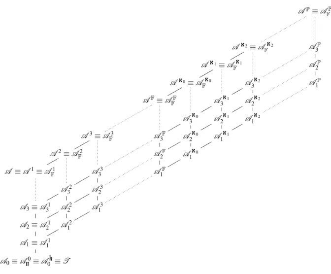
We can combine the ideas from Sections 3.1 and 3.2 to produce a family of modelsAnk, where:
• k is either a natural number k or infinite cardinal κ, indicating an upper bound on the size of
availability sets, or the symbol F indicating arbitrary finite availability sets are allowed, or the
symbolPindicating arbitrary availability sets are allowed;
• nis either a natural numbern, indicating an upper bound on the number of availability sets between
successive standard events, or the symbolFindicating any finite number is allowed.
Ifk=0 orn=0 thenAnkis just the standard traces model. Further,An≡A1
n andAk≡AFk.
We can show that this family is ordered as the natural extension of the earlier (one-parameter) fami-lies; the relationship between the models is illustrated in Figure 1. In particular, these models are distinct for n,k 6=0. We can re-use several of the earlier examples to this end. Example 13 shows that for
eachk6=0
Ak
0 ≺A k 1 ≺A
k
2 ≺. . .≺A k
F.
The following example generalises Example 21.
Example 23 Letnandkbe positive natural numbers. LetAbe a set of sizen×k+1. Consider
P = ?a:A→STOP,
Q =
⊓
B⊂A?a:B→STOP.
LetA1, . . . ,An,{a}be a partition ofA, where eachAiis of sizek. Thenhoffer A1, . . . ,offer An,aiis a trace ofPbut not ofQ, so these processes are distinguished byAk
n. However, the two processes are equivalent inAnk−1. HenceAnk−1≺Ank. Further, AnF distinguishes these processes, for all (finite) nand k, so Ak
n ≺A
F
n .
Example 19 shows thatAF
n ≺Anκfor each infinite cardinalκand for eachn. Further, Example 22 shows
that ifλ<κare two infinite cardinals, thenAnλ ≺Anκ≺AnP.
4
Discussion
Simulation and model checking The models described in this paper are not supported by the model
AP
≡AP F
Aℵ2≡Aℵ2
F A
P
3
Aℵ1≡Aℵ1
F q q q q q AP 2
Aℵ0≡Aℵ0
F q q q q q
Aℵ2
3 A
P
1
AF
≡AF F q q q q q
Aℵ1 3
q q q q
Aℵ2 2
Aℵ0 3
q q q q
Aℵ1 2
q q q q
Aℵ2 1
A3≡A3
F A F 3 q q q q
Aℵ0 2
q q q q
Aℵ1 1
q q q q
A2≡A2
F q q q q q AF 2 q q q q
Aℵ0 1
q q q q
A ≡A1≡AF1
q q q q A3 3 A F 1 q q q q A2 3 q q q q q A3 2
A3≡A1
3 q q q q A2 2 q q q q q A3 1
A2≡A1 2 q q q q A2 1 q q q q q
A1≡A1 1
q q q q
A0≡An0≡Ak
0 ≡T
Figure 1: The hierarchy of models
simulate the actionoffer A. For example,P=a→STOP✷b→STOPwould be simulated by
Psim = a→STOPsim✷b→STOPsim✷offer?A:P({a,b})→Psim,
STOPsim = offer.{} →STOPsim.
This simulation process, then, has the same traces as the original process in the Availability Sets Model, but with eachoffer Aaction replaced byoffer.A. The semantics in each of the other models can be obtained by restricting the size or number ofofferevents.
In [16], Roscoe shows that any operational semantics that is CSP-like, in a certain sense, can be simulated using standard CSP operators. One can define the operational semantics of the corrent paper in a way that makes them CSP-like, in this sense. Roscoe’s simulation is supported by a tool by Gibson-Robinson [3], which has been used to automate the simulation of the Singleton Availability Model and Availability Sets Model. This opens up the possibility of using FDR to perform analyses in these models.
incomparable with the Stable Failures Model. In fact, this example shows that all of the models in this paper except the Traces Model are incomparable with all of the models in Roscoe’s hierarchy except the Traces Model (so including the Ready Trace Model [11] and the Refusal Testing Model [9]); it is, perhaps, surprising that the hierarchies are so unrelated.
We believe that we could easily adapt our models to extend any of the finite linear observation models from [15], so as to obtain a hierarchy similar to that in Figure 1: in effect, the consideration of availability information is orthogonal to the finite linear observations hierarchy. Further, we have not considered divergences within this paper. We believe that it would be straightforward to extend this work with divergences, either building models that are divergence-strict (like the traditional Failures-Divergences Model [6, 13]), or non-divergence-strict (like the model in [14]).
In [5, 4], van Glabbeek considers a hierarchy of different semantic models in the linear time– branching time spectrum. Several of the models correspond to standard finite linear observation models, discussed above. One other model of interest is simulation.
Definition 24 [5] Asimulationis a binary relationRon processes such that for all eventsa, ifP R Qand P−→a P′, then for someQ′, Q−→a Q′ andP′R Q′. ProcessPcan be simulated byQ, denotedP→⊂ Qif there is a simulationRwithP R Q.PandQaresimilarifP→⊂ QandQ→⊂ P.
IfP→⊂ QandP7−→tr Pthen one can show thatQ
tr
7−→P, by induction on the length oftr. Hence ifPandQ
are similar, they are equivalent in the Availability Sets Traces Model, and hence all our other models. Simulation is strictly finer than our models, since it distinguishesa→b→c→STOP✷a→b→d→
STOPanda→(b→c→STOP✷b→d→STOP), for example.
A further possible class of models that we hope to investigate would record events that were available as alternatives to the events that were actually performed, and that were available from thesame stateas the events that were performed. For example, such a model would distinguish
P = a→c→STOP✷b→STOP
Q = (a→STOP✷b→STOP)⊲a→c→STOP,
sincePcan performha,ci, withbavailable from the state whereawas performed; butQdoes not have such a behaviour. Note that these two processes are equivalent in all the other availability models in this paper.
Two further possible directions in which this work could be extended would be (A) to record what events arenotavailable, or (B) to record thecompleteset of events that are available. We see considerable difficulties in producing such models. To see why, consider the processa→P. There are two different ways of viewing this process (which amount to different operational semantics for this process):
• One view is that the eventabecomes availability immediately. With this view: in model A, one cannot initially observe the unavailability ofa; in model B, the initial complete availability set is{a}. However, under this view, the fixed point theory does not work as required, sincedivis not the bottom element of the subset ordering: in model A,divhasainitially unavailable; in model B, div’s initial complete availability set is {}; these are both behaviours not exhibited by a→P. Further, under this view, nondeterminism is not idempotent, since, for example,a→P⊓a→P hasaunavailable initially; one consequence is that the proof of the no-junk result cannot be easily adapted to this view.
can initially observe the unavailability ofa; in model B, the initial complete availability set is{}. However, under this view, it turns out that the state of a→Pafter the a has become available cannot be expressed in the syntax of the language; this means that the proof of the no-junk result cannot be easily adapted to this view. (Proving a full abstraction result is straightforward, though.)
As noted in the introduction, in [7] we considered models for an extended version of CSP with a construct “if readyathenPelseQ”. This construct tests whether or not its environment offersa, so the model has much in common with model A above (and was built following the second view). As such, it did not have a no-junk result. Further, it did not have a full abstraction result, since it distinguished if readyathenPelsePandP, but no reasonable test would distinguish these processes.
Acknowledgements I would like to thank Bill Roscoe, Tom Gibson-Robinson and the anonymous
referees for useful comments on this work.
References
[1] C. Bolton & G. Lowe (2004):A Hierarchy of Failures-Based Models. Electr. Notes Theor. Comput. Sci.96, pp. 129–152.
[2] Formal Systems (Europe) Ltd (2005):Failures Divergence Refinement—User Manual and Tutorial. Version 2.8.2.
[3] T. Gibson-Robinson (2010):Tyger: A Tool for Automatically Simulation CSP-Like Languages in CSP. Mas-ter’s thesis, Oxford University.
[4] R.J. van Glabbeek (1993):The Linear Time–Branching Time Spectrum II; The semantics of sequential sys-tems with silent moves (extended abstract). In: ProceedingsCONCUR’93,4thInternational Conference on
Concurrency Theory,Lecture Notes in Computer Science715, Springer Verlag, pp. 66–81.
[5] R.J. van Glabbeek (2001): The Linear Time–Branching Time Spectrum I; The Semantics of Concrete, Se-quential Processes. In: J.A. Bergstra, A. Ponse & S.A. Smolka, editors: Handbook of Process Algebra, chapter 1, Elsevier, pp. 3–99.
[6] C. A. R. Hoare (1985):Communicating Sequential Processes. Prentice Hall.
[7] G. Lowe (2009):Extending CSP with tests for availability. In:Proceedings of Concurrent Process
Architec-tures.
[8] R. Milner (1980):A Calculus of Communicating Systems,LNCS92. Springer. [9] Abida Mukarram (1993):A Refusal Testing Model for CSP. D. Phil thesis, Oxford.
[10] R. de Nicola & M. C. B. Hennessy (1984): Testing Equivalences for Processes. Theoretical Computer
Science34, pp. 83–133.
[11] E. R. Olderog & C. A. R. Hoare:Specification-oriented Semantics for Communicating Processes. In: J. Diaz, editor:10th ICALP, LNCS 154, pp. 561–572.
[12] A. W. Roscoe (1994): Model-checking CSP. In: A Classical Mind, Essays in Honour of C. A. R. Hoare, Prentice-Hall.
[13] A. W. Roscoe (1997):The Theory and Practice of Concurrency. Prentice Hall.
[14] A. W. Roscoe (2005):Seeing beyond divergence. In:Proceedings of “25 Years of CSP”, LNCS 3525. [15] A. W. Roscoe (2009):Revivals, stuckness and the hierarchy of CSP models.Journal of Logic and Algebraic
Programming78(3), pp. 163–190.