www.atmos-meas-tech.net/8/4013/2015/ doi:10.5194/amt-8-4013-2015
© Author(s) 2015. CC Attribution 3.0 License.
Predicting ambient aerosol thermal–optical reflectance
measurements from infrared spectra: elemental carbon
A. M. Dillner1and S. Takahama2
1University of California – Davis, Davis, California, USA
2École polytechnique fédérale de Lausanne, Lausanne, Switzerland
Correspondence to:A. M. Dillner ([email protected]) and S. Takahama ([email protected])
Received: 18 March 2015 – Published in Atmos. Meas. Tech. Discuss.: 23 June 2015 Revised: 14 September 2015 – Accepted: 17 September 2015 – Published: 2 October 2015
Abstract.Elemental carbon (EC) is an important constituent of atmospheric particulate matter because it absorbs solar ra-diation influencing climate and visibility and it adversely af-fects human health. The EC measured by thermal methods such as thermal–optical reflectance (TOR) is operationally defined as the carbon that volatilizes from quartz filter sam-ples at elevated temperatures in the presence of oxygen. Here, methods are presented to accurately predict TOR EC using Fourier transform infrared (FT-IR) absorbance spec-tra from atmospheric particulate matter collected on poly-tetrafluoroethylene (PTFE or Teflon) filters. This method is similar to the procedure developed for OC in prior work (Dillner and Takahama, 2015). Transmittance FT-IR analy-sis is rapid, inexpensive and nondestructive to the PTFE filter samples which are routinely collected for mass and elemental analysis in monitoring networks. FT-IR absorbance spectra are obtained from 794 filter samples from seven Interagency Monitoring of PROtected Visual Environment (IMPROVE) sites collected during 2011. Partial least squares regression is used to calibrate sample FT-IR absorbance spectra to col-located TOR EC measurements. The FT-IR spectra are di-vided into calibration and test sets. Two calibrations are de-veloped: one developed from uniform distribution of sam-ples across the EC mass range (Uniform EC) and one devel-oped from a uniform distribution of Low EC mass samples (EC <2.4 µg, Low Uniform EC). A hybrid approach which
applies the Low EC calibration to Low EC samples and the Uniform EC calibration to all other samples is used to pro-duce predictions for Low EC samples that have mean error on par with parallel TOR EC samples in the same mass range and an estimate of the minimum detection limit (MDL) that is on par with TOR EC MDL. For all samples, this hybrid
approach leads to precise and accurate TOR EC predictions by FT-IR as indicated by high coefficient of determination (R2; 0.96), no bias (0.00 µg m−3, a concentration value based
on the nominal IMPROVE sample volume of 32.8 m3), low
error (0.03 µg m−3) and reasonable normalized error (21 %).
These performance metrics can be achieved with various de-grees of spectral pretreatment (e.g., including or excluding substrate contributions to the absorbances) and are compa-rable in precision and accuracy to collocated TOR measure-ments. Only the normalized error is higher for the FT-IR EC measurements than for collocated TOR. FT-IR spectra are also divided into calibration and test sets by the ratios OC/EC and ammonium/EC to determine the impact of OC and am-monium on EC prediction. We conclude that FT-IR analysis with partial least squares regression is a robust method for accurately predicting TOR EC in IMPROVE network sam-ples, providing complementary information to TOR OC pre-dictions (Dillner and Takahama, 2015) and the organic func-tional group composition and organic matter estimated pre-viously from the same set of sample spectra (Ruthenburg et al., 2014).
1 Introduction
ar-eas of the USA, the Speciation Trends Network/Chemical Speciation Network (Flanagan et al., 2006) in urban ar-eas of the USA, and the European Monitoring and Evalu-ation Programme (EMEP; Torseth et al., 2012) throughout Europe. These regional multi-year data sets are useful for observing trends in particulate concentrations (Hand et al., 2013; Hidy et al., 2014; Torseth et al., 2012) and visibil-ity (Hand et al., 2014), evaluating aerosol transport models (Mao et al., 2011), constraining climate models (Liu et al., 2012) and assessing health impacts (Krall et al., 2013). EC is measured using thermal–optical methods such as thermal– optical reflectance (TOR) (Chow et al., 2007), NIOSH 5040 (Birch and Cary, 1996) and European Supersites for Atmo-spheric Aerosol Research (EUSAAR-2 protocol; Cavalli et al., 2010), in which particles collected on quartz filters are subjected to a temperature gradient, first in an inert envi-ronment and then in an oxidizing envienvi-ronment (Chow et al., 2007). Organic carbon (OC) and EC are operationally de-fined by the temperature and environmental conditions under which the carbon evolves from the aerosol sample. Charred organic material is subtracted from the measured EC based on laser reflectance or transmittance (Cavalli et al., 2010; Chow et al., 2007). These thermal–optical methods are not applicable to the PTFE (polytetrafluoroethylene) media used for gravimetric mass, elemental composition and sometimes light absorption in sampling networks because the filter ma-terial is unstable at high temperatures. TOR methods are also destructive to the sample and expensive.
Thermal–optical methods are one type of method that seeks to measure carbon in atmospheric aerosols that is struc-turally similar to graphite in that it is composed ofsp2bonds
and is strongly light absorbing (Bond and Bergstrom, 2006). Thermal–optical methods refer to this material as EC. Other methods use light absorption to characterizesp2-bonded
car-bon in aerosol (Andreae and Gelencsér, 2006) and typi-cally refer to the constituent being measured as black car-bon (BC). Continuous light absorption measurements are made by such instruments as the PSAP (Bond et al., 1999), aethalometer (Collaud Coen et al., 2010) and multi-angle ab-sorption photometer (Petzold et al., 2005). Time-integrated absorption measurements are made from filter samples us-ing instruments such as the hybrid-integratus-ing plate method used by the IMPROVE network (White et al., 2015). Fourier transform infrared (FT-IR) spectroscopy has also been used to characterize sp2-bonded carbon in particles and other
environmental samples. FT-IR spectra of ground graphite and activated carbon have prominent peaks at 1580 cm−1
which were assigned to the graphitic structure of the material (Friedel and Carlson, 1971). FT-IR spectra of ground char-coal and synthetic and marine sediments had similar peaks at 1580 cm−1 and additional peaks at 1720 and 1240 cm−1,
which were assigned to carbonyl and single carbon–oxygen bonds, respectively (Smith et al., 1975). FT-IR and partial least squares regression (PLSR) have been used to quantify BC in soil samples by measuring benzene polycarboxylic
acids, which are aromatic markers for black carbon (Borne-mann et al., 2007). In a companion paper (Takahama et al., 2015), we will discuss similarities and differences in the vi-brational modes identified by these previous authors relevant for quantitative prediction in atmospheric elemental carbon. However, the presence of wave numbers that correlate to TOR EC indicates the potential for FT-IR spectra calibrated to TOR EC using PLSR to predict TOR EC in aerosol sam-ples.
In this work, FT-IR spectra are calibrated to TOR EC us-ing PLSR, similar to our previous method for predictus-ing TOR OC (Dillner and Takahama, 2015). PLSR is a general method that has been used to calibrate FT-IR spectra of environmen-tal samples such as dust (Weakley et al., 2014), food (Polshin et al., 2011) and soil (Bornemann et al., 2007) to constituents of interest. As described above, thermal–optical methods cur-rently provide EC measurements in air monitoring network ambient particle matter samples. Such networks simultane-ously sample particles on PTFE filters which are used for gravimetric mass and elemental composition analysis and can also be used to obtain FT-IR spectra. In this work, EC is predicted from infrared spectra of PTFE filter samples of aerosols using PLSR. The methods are developed and tested using EC from TOR analysis and FT-IR spectra from parallel PTFE filters from 1 year of samples from seven IMPROVE sites.
2 Methods
2.1 IMPROVE network samples
This study uses 794 IMPROVE particulate matter samples collected on PTFE filters and 54 blank PTFE filters. The IM-PROVE samples were collected at seven sites during 2011 (Fig. S1 in the Supplement). These are the same samples, blanks and consequent FT-IR spectra used for developing the OC method in Dillner and Takahama (2015) and the organic matter/organic carbon method in Ruthenburg et al. (2013). Additional details are provided in these papers. In the IM-PROVE network, filter samples of particles less than 2.5 µm (PM2.5) are collected every third day from midnight to
mid-night local time at a nominal flow rate of 22.8 liters per minute, which yields a nominal volume of 32.8 m3.
The FT-IR analysis is applied to 25 mm PTFE filters (Teflon, Pall Gelman, 3.53 cm2 sample area) that are
ana-lyzed for gravimetric mass, elements and light absorption in the IMPROVE network. Quartz filters collected in parallel with the PTFE filters are analyzed by TOR and adjusted to account for charring of organic material prior to reporting EC mass in the IMPROVE network (Chow et al., 2007). For this work, the EC values are also adjusted to account for flow differences between the quartz and PTFE filters.
In order to provide reference performance metrics for the evaluation of the FT-IR to TOR comparisons (see Sect. 2.4 for a description of the metrics), measurements from seven IMPROVE sites with collocated TOR measurements (Ever-glades, Florida; Hercules Glade, Missouri; Hoover, Califor-nia; Medicine Lake, Montana; Phoenix, Arizona; Saguaro West, Arizona; Seney, Michigan) are used.
2.2 FT-IR analysis 2.2.1 Spectra acquisition
PTFE filters are analyzed using a Tensor 27 FT-IR spec-trometer (Bruker Optics, Billerica, MA) equipped with a liq-uid nitrogen-cooled wide-band mercury cadmium telluride detector. The samples are analyzed using transmission FT-IR over the mid-infrared wave number region of 4000 to 420 cm−1 (Ruthenburg et al. (2014) describes the protocol
in further detail). Absorbance spectra are calculated using a recent spectrum of the empty sample compartment as a zero reference. Air free of water vapor and carbon dioxide (de-livered by purge-gas generator; PureGas LLC, Broomfield, CO) is used to continuously purge the optical compartments of the instrument and to purge the sample compartment for 4 min before each sample or reference spectrum is acquired.
2.2.2 Spectra preparation
Three different versions of the absorption spectra are used in our analysis (Fig. S2), corresponding to different pre-treatments and wavelength selection. (1) “Raw” spectra are
unmodified spectra except that values interpolated during the zero-filling process are removed. These spectra contain all 2784 wave numbers. (2) “Baseline-corrected” spectra in-clude absorbances above 1500 cm−1and the substrate
con-tribution is removed by subtracting an average blank filter spectrum and then using linear or polynomial baselines by spectral region as described by Takahama et al. (2013). These spectra are standardized to a 2 cm−1resolution and so
con-tain 1563 wave numbers. (3) “Truncated” spectra are the raw spectra interpolated to match the wave numbers in the baseline-corrected spectra, which excludes the PTFE peaks (the region below 1500 cm−1) and so also contain 1563 wave
numbers.
2.3 Calibration
The FT-IR spectra are calibrated to TOR EC measurements using PLSR using the kernel pls algorithm, implemented by the pls library (Mevik and Wehrens, 2007) for the R statisti-cal package (R Core Team, 2014). Conceptual description of PLSR can be found in Dillner and Takahama (2015), Taka-hama et al. (2015) and Ruthenburg et al. (2014) and refer-ences therein. Briefly, in PLSR the matrix of spectra is de-composed into factors and their respective weights. Candi-date models are generated by varying the number of factors used to reconstruct the EC mass in the calibration filters.
Using the common approach for model selection and as-sessment (Hastie et al., 2009; Bishop, 2006; Witten et al., 2011), two-thirds of the 794 samples and two-thirds of the blanks filters (which are assumed to have 0 EC mass) are used for developing the calibration and one-third of the sam-ples and blanks (called the test set) are used to evaluate the model. Ambient samples with EC below TOR EC MDL are excluded from the model so as not to train the calibration with samples that have a low signal-to-noise ratio.K-fold
cross validation withk=10 is used to estimate the accuracy
of each candidate model. The minimum root mean square er-ror of cross validation (Mevik and Cederkvist, 2004) is used to select the model with the least prediction error. This proce-dure permits development and selection of PLSR models us-ing only the samples in the calibration set and guards against over-fitting to a single set of samples. The test set, which has not been used in model development or selection, is used for model evaluation.
0.0 0.5 1.0
Prob
. density (a.u.)
Uniform ● ● ● ● ● ● ● ● ● ● −0.3 −0.2 −0.1 0.0 0.1 0.2 0.3 Bias ( µ g m 3) ● ● ● ● ● ● ● ● ● ●
0 10 20 30
0 10 20 30 40 50 60 70 Nor maliz
ed error (%)
Non−uniform A ● ● ● ● ● ● ● ● ● ● ● ● ● ● ● ●
0 10 20 30
Non−uniform B ● ● ● ● ● ● ● ● ● ● ● ● ● ● ● ●
0 10 20 30
Non−uniform C ● ● ● ● ● ● ● ● ● ● ● ●
0 10 20 30
EC(µg)
● Spectra type raw baseline corrected truncated ● ● ● Median EC(µg)
0−2.4 2.4−10 10−20 ● ● Set calibration test
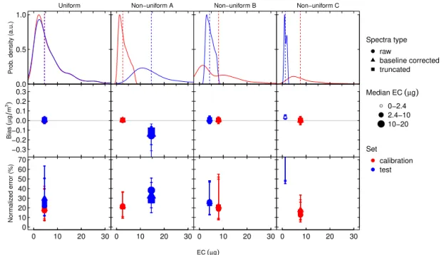
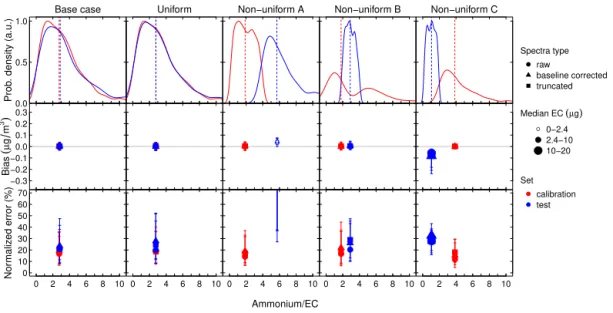
Figure 1.Uniform and Nonuniform EC calibrations. The probability density distribution of EC and bias and normalized error (with the
interquartile range shown by error bars) in the calibration (red) and test (blue) sets for the Uniform EC case and three Nonuniform EC cases. Vertical lines are the median of the EC mass distributions color-coded for calibration and test sets.
iteration of the cross-validation process has a roughly consis-tent number of blanks used for calibration. Calibrations de-veloped without ordering the blanks and without interspers-ing the blanks in the calibration filter set lead to inconsistent MDL values.
EC is predicted for a sample (i) by taking the product of
the absorbance at wave numberj (xi,j) and the calibration
vector (bj) as shown in Eq. (1).
ECi= X
j
xi,jbj (1)
Blank samples in the test set are used to calculate the MDL. Multiple calibrations are developed by varying the spectra type used and by selecting filters for the calibration and test sets using different ordering regimes. Initially, we develop a set of calibrations based on uniform and nonuniform distri-butions of EC in the calibration and test sets. For the Uni-form case, the samples are ordered by EC mass and every third sample is put into the test set so the distribution of EC is the same in the calibration and test sets. Three Nonuniform cases are developed to assess the impact of EC distribution on the quality of the calibration. For the Nonuniform cases, the samples are ordered by EC mass and then selected for calibration and test set based on where each samples falls within the range of EC masses. The three Nonuniform cases are: (1) samples with mass in the highest two-thirds of the EC mass range are used for calibration and samples with EC in the lowest third of the EC mass range are used as the test set (Nonuniform A); (2) samples in the highest and lowest third of the EC mass range are used to predict samples in
the middle third of the EC mass range (Nonuniform B); and (3) samples with EC mass in the lowest two-thirds of the EC range are used to predict samples in the highest third of the EC mass range (Nonuniform C).
Figure 1 shows the Uniform and three Nonuniform cali-brations developed for EC. A description of the performance metrics shown in Fig. 1 are given in Sect. 2.4. The top row gives the EC distribution of the test and calibration set for each case. The EC distributions reflect the algorithm used to select the filters for that case. The median and 25th to 75th percentiles (interquartile range) of the bias and normal-ized error are shown in the lower two rows of Fig. 1 for each of the three spectra types (indicated by symbol shape). Small open symbols are used for sets with low median EC masses. Larger closed symbols have higher median EC masses. The EC distributions for the Uniform case shows that the dis-tribution of samples in the calibration set and test set are very similar. This leads to predictions with small bias (mid-dle plot) and median normalized errors (bottom plot) ranging from 15 to 30 % for the test and calibration sets for the three spectral treatments. However, when low EC mass samples are used to predict high EC samples (Nonuniform A) and high samples are used to predict low EC samples (Nonuni-form C), the test set is biased, leading to high error, especially when the EC values are low (Nonuniform C).
In order to eliminate bias in the calibration and improve prediction capability for Low EC samples, we develop a lo-calized calibration for samples in the lowest third of the EC mass range (EC<2.4 µg). The Low Uniform EC calibration
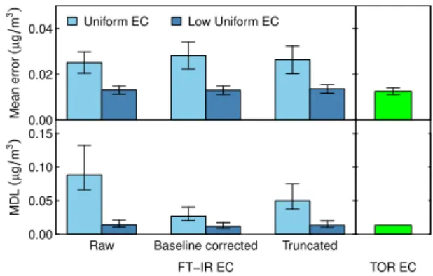
that are in the lowest third of the EC mass range to pre-dict samples in the test set that are also in the lowest third of the EC mass range. Localization of the calibration is a commonly used method to improve the performance of the calibration, often at the more difficult to measure low end of the range. The Uniform (which contains samples across the whole range of EC; Fig. 1) and Low EC calibrations are used to predict Low EC test set samples and the resulting error and MDL are compared in Fig. 2. The mean error or pre-cision of collocated TOR EC samples below 2.4 µg and the reported TOR EC MDL are also shown in Fig. 2. The Low EC calibration reduces the error for all three spectral types to a value similar to that of the precision of collocated TOR EC samples in the same mass range. In addition, the MDL (which is based on the prediction of blank filters) is reduced to approximately the TOR MDL for all three spectral types. This comparison indicates that a localized calibration greatly improves the prediction quality for Low EC samples and that the error in the FT-IR prediction is due primarily to TOR EC measurement uncertainty.
A hybrid calibration method, which includes the Uniform calibration for the whole EC range and the Low EC calibra-tion for the Low EC range is used for all results presented in Sect. 3, regardless of the ordering scheme used to select fil-ters for the calibration and test sets. In the hybrid calibration method, the Uniform calibration is used to predict all filters in the test set. Those filters in the test set which are predicted to be in the lowest third of the EC mass are then analyzed by the Low EC calibration. The prediction from the full calibra-tion is used for samples above the lowest third and predic-tions from the Low EC calibration are used for the Low EC samples.
A “Base case” hybrid calibration, in which the samples are chronologically stratified per site (i.e., ordered by date for each site), is developed as a reference scenario. Every third sample in the ordered list is put into the test set and the rest are put into the calibration set. The Base case has the same samples in the test set as the Base case for the OC predictions reported earlier (Dillner and Takahama, 2015). Description of a minor error in the OC calibration set for the Base case is documented in Sect. S3, and this has been corrected for the EC calculations in this work. The blanks are calculated and distributed as previously stated. This ordered set of samples based on sites and date provides fairly uniform distribution of EC and aerosol composition in the calibration and test sets. In addition to the Base case, Uniform and Nonuniform OC/EC, ammonium/EC and site-specific calibrations are developed using the hybrid approach and discussed in more detail in the Sect. 3.
2.4 Methods for evaluating of the quality of calibration The quality of each calibration is evaluated by calculating four performance metrics: bias, error, normalized error and the coefficient of determination (R2) of the linear regression
0.00 0.02
0.04 Uniform EC Low Uniform EC
Mean error
(
µ
g
m
3)
Raw Baseline corrected Truncated 0.00
0.05 0.10 0.15
MDL
(
µ
g
m
3)
FT−IR EC TOR EC
Figure 2.Mean error of a Low EC test set (EC<2.4 µg) and MDL
from the Uniform EC and Low Uniform EC calibrations. The same Low EC test set is predicted by the Uniform and Low Uniform cal-ibrations. The mean error of collocated EC samples less than 2.4 µg and the reported EC MDL for the TOR method are shown for com-parison.
fit of the predicted FT-IR EC to measured TOR EC. FT-IR EC is the EC predicted from the FT-IR spectra and the PLSR calibration model. The bias is the median difference between measured (TOR EC) and predicted FT-IR EC for the test set. Error is the median absolute bias. The normalized error for a single prediction is the error divided by the TOR EC value. The median normalized error is reported. The performance metrics are also calculated for the collocated TOR observa-tions and compared to those of the FT-IR EC to TOR EC regression. The MDL and precision of the FT-IR method are calculated and compared to the reported MDL and calculated precision of the TOR method. The MDL of the FT-IR method is 3 times the standard deviation of the blanks in the test set (18 blank filters). MDL for the TOR method is 3 times the standard deviation of 514 blanks (Desert Research Intitute, 2012). Precision for both FT-IR and TOR are calculated us-ing the 14 parallel samples in the test set at the Phoenix, AZ, site.
3 Results
3.1 Predicting TOR EC from infrared spectra
Using the hybrid calibration with the Base case scenario, Fig. 3 shows the prediction of the calibration samples and the test set samples along with the collocated TOR samples with the same EC distribution. The calibration and test sets are predicted with no bias (nonlinearity is removed by using the Low EC calibration) and have similar error, normalized error andR2. The precision between TOR samples is expected to
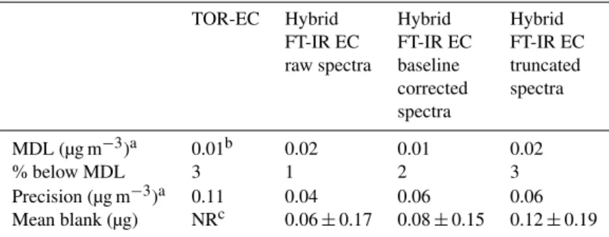
Table 1.MDL and precision for Hybrid FT-IR EC and TOR EC.
TOR-EC Hybrid Hybrid Hybrid
FT-IR EC FT-IR EC FT-IR EC
raw spectra baseline truncated
corrected spectra
spectra
MDL (µg m−3)a 0.01b 0.02 0.01 0.02
% below MDL 3 1 2 3
Precision (µg m−3)a 0.11 0.04 0.06 0.06
Mean blank (µg) NRc 0.06±0.17 0.08±0.15 0.12±0.19
aConcentration units of µg m−3for MDL and precision are based on the IMPROVE volume of
32.8 m3.bValue reported for network (0.44 µg) in concentration units.cNot reported.
Bias=0.00 µg m3 Error=0.03 µg m3 Norm. Error=19% R2=0.98
0 20 40 60 80 100
0 20 40 60 80
100 (a) Calibration set
Bias=0.00 µg m3 Error=0.03 µg m3 Norm. Error=21% R2=0.96
0 20 40 60 80 100
(b) Test set
TOR EC(µg)
FT−IR EC
(
µ
g
)
Bias=−0.00 µg m3 Error=0.02 µg m3 Norm. Error=13% R2=0.97
0 20 40 60 80 100
0 20 40 60 80
100 (c) Collocated TOR
TOR EC(µg)
Collocated T
OR EC
(
µ
g
)
Figure 3.Predicted EC for calibration set(a)and test set(b)for the Base case using a hybrid calibration model. The collocated TOR
samples(c)are from sites with parallel quartz filters that are both analyzed by TOR. Only the Phoenix site has samples in the calibration, test
and collocated data sets. There are 521 samples in the calibration set(a), 265 samples in the test set(b)and 431 samples in the collocated
TOR data set(c). Concentration units of µg m−3for bias and error are based on the IMPROVE nominal volume of 32.8 m3.
collocated TOR EC precision. The distribution of normal-ized errors for the calibration and test set for the raw spectra case and the collocated precision for the TOR samples are quite similar (Fig. S4a). The Base case bias (0.00 µg m−3)
and absolute error (0.03 µg m−3) are on the same order as
the Base case for TOR OC (test set bias=0.02 µg m−3and
error=0.08 µg m−3; Dillner and Takahama, 2015) and the
R2values are the same (0.96; Dillner and Takahama, 2015).
The normalized error for the test set (21 %) is higher than the collocated TOR EC precision (13 %) and higher than the TOR OC normalized error (11 %). The hybrid calibra-tion also produces high-quality prediccalibra-tions of EC baseline-corrected and truncated spectra as indicated by the similarity in performance metrics for all three spectral types (Fig. S4b). The distribution of normalized errors for the calibration and test set for the baseline-corrected and truncated spectral treatments are similar to raw spectra and the collocated pre-cision for the TOR samples (Fig. S4a). Section S5 demon-strates that the number of samples in the calibration set can be reduced and still provide high-quality predictions. The analysis suggests that the accuracy of FT-IR EC predictions is comparable to the precision of collocated TOR EC mea-surements.
Table 1 gives the MDL and collocated Phoenix sample precision for the hybrid FT-IR EC predictions for each spec-tral type and TOR EC. The MDL for all hybrid FT-IR EC spectral types are approximately the same as TOR EC with 3 % or fewer of the samples below MDL. Section S5 shows that the MDL is independent of the number of blanks in-cluded in the calibration and the number of samples inin-cluded in the calibration set (from two-thirds to one-third of the samples). The collocated Phoenix precision is better for the FT-IR methods than for TOR by about half. The mean pre-dicted value for the blanks filters (last row of Table 1) is less than half of the first percentile of predicted EC values for the raw and baseline-corrected spectra and equivalent to the sec-ond percentile for the truncated case. The precision is on the same order for all three spectral types.
An alternate method for estimating EC is to predict to-tal carbon (TC=OC+EC) and subtract the OC prediction.
0.0 0.5 1.0
Prob
. density (a.u.)
Base case
● ●
−0.3 −0.2 −0.1 0.0 0.1 0.2 0.3
Bias
(
µ
g
m
3)
● ●
0 5 10 15 20 25 0
10 20 30 40 50 60 70
Nor
maliz
ed error (%)
Uniform
● ●
● ●
0 5 10 15 20 25
Non−uniform A
● ●
●
0 5 10 15 20 25
Non−uniform B
●●
● ●
0 5 10 15 20 25
Non−uniform C
●
●
●
●
0 5 10 15 20 25 OC/EC
●
Spectra type raw
baseline corrected truncated
●
●
●
Median EC(µg) 0−2.4 2.4−10 10−20
● ●
Set calibration test
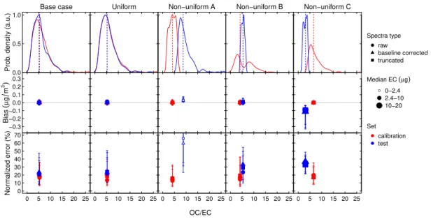
Figure 4.The probability distribution of OC/EC and bias and normalized error (with the interquartile range shown by error bars) in the
calibration (red) and test (blue) sets for five hybrid calibration cases: the Base case, the Uniform OC/EC case and three Nonuniform OC/EC cases. Vertical lines on the probability distributions are the color-coded median of the OC/EC distributions.
3.2 Evaluating causes of bias and error by selecting the calibration and test sets based on measured
parameters
In this section, we consider the role of aerosol composi-tion on the quantificacomposi-tion of EC. Aerosol composicomposi-tion is de-scribed by the distribution of OC/EC and ammonium/EC. In other work, we show that OC and EC measurements by FT-IR and PLSR rely on similar wavebands for predictions (Takahama et al., 2015). Therefore, OC could be considered an interferant to the measurement of EC. We evaluate this possible interferant using the ratio of OC to EC because the impact of OC is likely dependent on its mass relative to EC mass. Ammonium absorbs FT-IR radiation in the same wave number region as OC and EC and so can also be considered an interferant. We use the ratio of ammonium to EC mass loadings to isolate the effect of ammonium. OC/EC and am-monium/EC are not correlated to 1/EC (R2<0.2), which
in-dicates that impacts observed from EC, OC/EC and ammo-nium/EC are at least somewhat independent of each other. Therefore, separate calibrations were developed by ordering the samples by OC/EC and ammonium/EC.
As was done for Uniform EC case, samples are arranged in ascending order by the parameter of interest prior to selection of filters for the calibration and test sets. Every third sam-ple in the ordered list is put into the test set and the remain-ing samples are put into the calibration set. These cases are called the Uniform OC/EC case and Uniform ammonium/EC case. Three Nonuniform cases are also considered and the OC/EC Nonuniform cases are detailed here as an example: samples in the lowest two-thirds of the OC/EC range are used to predict samples in the highest third of the OC/EC range
(Nonuniform A); the highest and lowest third of the OC/EC range are used to predict the middle third OC/EC range (Nonuniform B); and the highest two-thirds of the OC/EC range are used to predict samples in the lowest third of the OC/EC range (Nonuniform C). All predictions are based on the hybrid calibration model (Sect. 3.1) such that Low EC samples in any of the test sets are predicted using a Low EC calibration developed for that case.
The top row of subplots in Fig. 4 shows that the distribu-tion of OC/EC in the test and calibradistribu-tion sets for the Base case and the Uniform OC/EC case are similar. The three Nonuniform OC/EC cases have distributions that are differ-ent for the test and calibrations sets. The Base and Uniform case have 0 bias and similar normalized error in the test and calibration sets indicating good predictions for these cases. When there is a large difference in OC/EC distribution be-tween the test and calibration sets (Nonuniform cases), the normalized error is higher and sometimes a bias is induced. For Nonuniform C, there is a significant negative bias and the normalized error is about 35 % (10 % higher than the cal-ibration set). For Nonuniform B, in which the medians are similar but the distribution of OC/EC is quite different be-tween the sets, there is less than 10 % higher error in the test set than the calibration set. For Nonuniform A, in which the median EC value is in the Low EC range, the median nor-malized error is at least 60 % and the range of error is high, which is due to both the difference in the chemical composi-tion of the aerosol in the test and calibracomposi-tion sets and the Low EC values.
0.0 0.5 1.0
Prob
. density (a.u.)
Base case
● ●
−0.3 −0.2 −0.1 0.0 0.1 0.2 0.3
Bias
(
µ
g
m
3)
● ●
0 2 4 6 8 10 0
10 20 30 40 50 60 70
Nor
maliz
ed error (%)
Uniform
● ●
● ●
0 2 4 6 8 10
Non−uniform A
● ●
●
0 2 4 6 8 10
Non−uniform B
●●
●●
0 2 4 6 8 10
Non−uniform C
●
●
●
●
0 2 4 6 8 10 Ammonium/EC
●
Spectra type raw
baseline corrected truncated
●
●
●
Median EC(µg) 0−2.4 2.4−10 10−20
● ●
Set calibration test
Figure 5.The probability distribution of ammonium/EC and bias and normalized error (with the interquartile range shown by error bars) in the calibration (red) and test (blue) sets for five hybrid calibration cases: the Base case, the Uniform ammonium/EC case and three Nonuniform ammonium/EC cases. Vertical lines on the probability distributions are the color-coded median of the ammonium/EC distributions.
have near 0 bias and low normalized error. The results for the Nonuniform A and C cases are very similar to the Nonuni-form A case for OC/EC. In the NonuniNonuni-form C case, the cal-ibration set contains a higher amount of ammonium and EC is under-predicted (some of the EC is assumed to be am-monium) in low ammonium/EC test samples (bias,−0.04 to −0.06 µg m−3) and the range in bias of individual samples
in-creases. The normalized error increases by about 15 % from the calibration set to the test set but the error bars are about the same for the two sets. When low ammonium/EC sam-ples are used to predict samsam-ples with high ammonium/EC (Nonuniform A), the normalized error becomes very large. This is due in part to the median EC value being below 2.4 µg. It is likely that additional error is induced because the cali-bration set is not trained to disregard ammonium in the pre-diction of EC, so some of the ammonium is reported to be EC leading to a positive bias and increased error. The dis-tribution of EC, OC/EC and ammonium/EC for the test and calibration sets for the Base, Uniform and Nonuniform cases are shown in Sect. S7. When the chemical composition, as in-dicated by OC/EC and ammonium/EC, is different between the calibration and test sets, the predictions have higher error than when the chemical compositions are similar.
3.3 Prediction of specific sites
Calibrations are developed using ambient samples for all but one site in the calibration set. The one site omitted from the calibration is predicted. Figure 6 shows the distributions of EC in the test and calibration set and the median and in-terquartile range of bias and normalized error for all sites. Three sites, Mesa Verde, Olympic and Trapper Creek, have median EC mass below 2.4 µg and, although the bias is near
0, they have the highest median (40 to 60 %) and range of normalized error. As shown with the Low EC calibration and comparison to collocated TOR samples (Sect. 3.1), these er-rors are similar to collocated precision of TOR samples in the same EC range, indicating that the error is due primarily to TOR analytical error. All other sites have higher EC mass and are expected to be predicted well, based on EC mass alone. However, only the Proctor Maple Research Facility is predicted well (Fig. 6). EC, OC/EC and ammonium/EC dis-tributions at the Proctor Maple Research Facility are similar to the calibration set. The increased errors for the remain-ing three sites, Phoenix, Sac and Fox and St. Marks, are due to differences in aerosol composition between the calibra-tion set and these sites. Distribucalibra-tions of EC, OC/EC and am-monium/EC for the test and calibration sets for all sites are shown in Sect. S7.
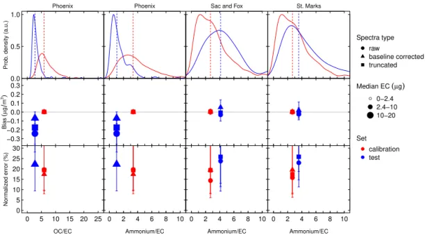
Figure 7 shows the OC/EC and ammonium/EC distribu-tions at Phoenix and the ammonium/EC distribudistribu-tions for Sac and Fox and St. Marks. Phoenix, an urban site, has higher EC than the rural sites (Fig. 6). Phoenix also has lower OC/EC than the other sites (OC/EC Nonuniform C) and has lower ammonium/EC than the rural sites (ammonium/EC Nonuni-form C). All of these compositional differences lead to a neg-ative bias and increased error as seen in the Phoenix samples (bias up to 0.03 µg m−3 and error up to 50 %). All six
0.0 0.5 1.0
Prob
. density (a.u.)
Mesa Verde
● ●
−0.3 −0.2 −0.1 0.0 0.1 0.2 0.3
Bias
(
µ
g
m
3)
● ●
0 10 20 30 0
10 20 30 40 50 60 70
Nor
maliz
ed error (%)
Olympic
● ●
● ●
0 10 20 30
Phoenix
●
●
●
●
0 10 20 30
Proctor Maple RF
●●
●●
0 10 20 30
Sac and Fox
●●
● ●
0 10 20 30
St. Marks
●●
● ●
0 10 20 30
Trapper Creek
● ●
● ●
0 10 20 30 EC(µg)
●
Spectra type raw
baseline corrected truncated
●
●
●
Median EC(µg) 0−2.4 2.4−10 10−20
● ●
Set calibration test
Figure 6.The distribution of EC and bias and normalized error (with the interquartile range shown by error bars) in the calibration (red) and test (blue) sets for calibrations developed for each site. Vertical lines are the median of the EC mass distributions color-coded for calibration and test sets.
0.0 0.5 1.0
Prob
. density (a.u.)
Phoenix
●
●
−0.3 −0.2 −0.1 0.0 0.1 0.2 0.3
Bias
(
µ
g
m
3)
●
0 5 10 15 20 25 0
5 10 15 20 25 30
Nor
maliz
ed error (%)
OC/EC
Phoenix
●
●
●
0 2 4 6 8 10
Ammonium/EC
Sac and Fox
● ●
● ●
0 2 4 6 8 10
Ammonium/EC
St. Marks
●●
● ●
0 2 4 6 8 10
Ammonium/EC
● Spectra type
raw
baseline corrected truncated
●
●
● Median EC(µg)
0−2.4 2.4−10 10−20
●
● Set
calibration test
Figure 7.The distribution of OC/EC and bias and normalized error (with the interquartile range shown by error bars) in the calibration (red) and test (blue) sets for calibrations developed for Phoenix and the distribution of ammonium/EC, bias and normalized error for Phoenix, Sac and Fox and St. Marks. Vertical lines are the median of the distributions color-coded for calibration and test sets.
compared to the calibration set likely due to ammonium/EC differences.
We can therefore estimate how well a site not included in the calibration will be predicted based on the EC, OC/EC and ammonium/EC for the site. For sites with low EC mass, the error ranges from 40 to 60 %. Phoenix, which has higher EC, lower OC/EC and lower ammonium/EC than the rural sites, has biased predictions and error between 20 and 50 %. Differences in ammonium/EC alone produce higher errors
up to 40 % for Sac and Fox and St. Marks, especially for the truncated spectral type.
4 Conclusions
are used in partial least squares regression to develop calibra-tions to predict TOR EC. A hybrid approach is used for cali-bration in which samples with Low EC are calibrated with a Low EC calibration and all other samples are calibrated with a calibration that spans the range of EC samples (a descrip-tion of steps for calibradescrip-tion are included in the Supplement). The Low EC calibration produces predictions with mean er-ror similar to that of collocated TOR samples in the same mass range and similar MDLs, indicating that the errors in the FT-IR method are primarily due to TOR measurement un-certainty. All three spectral types produce high-quality pre-dictions. The hybrid calibrations developed from samples ordered by site date (Base case), EC, OC/EC and ammo-nium/EC, produce nearly bias-free predictions with low er-ror (∼0.02 µg m−3or 20–25 %). Blank filters in the test set
are used to calculate MDL, but the number of blanks in the calibration set does not impact the value of the MDL. Using a calibration set that does not have similar composition to the test set (i.e., using samples in the calibration set that do not span the full range of EC, OC/EC or ammonium/OC) leads to higher bias and errors and is not recommended for obtaining high-quality predictions. In the proposed method, error and bias are kept to a minimum by including samples in the cal-ibration set that have a similar composition as the test set, as indicated by EC, OC/EC and ammonium/EC. Therefore, we conclude that FT-IR spectra calibrated to TOR EC using par-tial least squares regression is a robust method for predicting TOR elemental carbon from particulate matter samples. Fu-ture work includes establishing that the calibration developed here can be used to predict TOR EC for samples collected during other years and developing a calibration that includes samples with a broader range of aerosol composition.
The Supplement related to this article is available online at doi:10.5194/amt-8-4013-2015-supplement.
Acknowledgements. The authors acknowledge funding from the IMPROVE program and EPA (National Park Service cooperative agreement P11AC91045) and EPFL startup funding.
Edited by: P. Herckes
References
Andreae, M. O. and Gelencsér, A.: Black carbon or brown car-bon? The nature of light-absorbing carbonaceous aerosols, At-mos. Chem. Phys., 6, 3131–3148, doi:10.5194/acp-6-3131-2006, 2006.
Birch, M. E. and Cary, R. A.: Elemental carbon-based method for occupational monitoring of particulate diesel exhaust: Methodology and exposure issues, Analyst, 121, 1183–1190, doi:10.1039/an9962101183, 1996.
Bishop, C.: Pattern recognition and machine learning, Springer-Verlag, New York, 2006.
Bond, T. C. and Bergstrom, R. W.: Light absorption by carbona-ceous particles: An investigative review, Aerosol Sci. Tech., 40, 27–67, doi:10.1080/02786820500421521, 2006.
Bond, T. C., Anderson, T. L., and Campbell, D.: Calibration and intercomparison of filter-based measurements of visible light absorption by aerosols, Aerosol Sci. Tech., 30, 582–600, doi:10.1080/027868299304435, 1999.
Bond, T. C., Doherty, S. J., Fahey, D. W., Forster, P. M., Berntsen, T., DeAngelo, B. J., Flanner, M. G., Ghan, S., Karcher, B., Koch, D., Kinne, S., Kondo, Y., Quinn, P. K., Sarofim, M. C., Schultz, M. G., Schulz, M., Venkataraman, C., Zhang, H., Zhang, S., Bellouin, N., Guttikunda, S. K., Hopke, P. K., Jacobson, M. Z., Kaiser, J. W., Klimont, Z., Lohmann, U., Schwarz, J. P., Shindell, D., Storelvmo, T., Warren, S. G., and Zender, C. S.: Bounding the role of black carbon in the climate system: A sci-entific assessment, J. Geophys. Res.-Atmos., 118, 5380–5552, doi:10.1002/jgrd.50171, 2013.
Bornemann, L. C., Kookana, R. S., and Welp, G.: Differential sorp-tion behaviour of aromatic hydrocarbons on charcoals prepared at different temperatures from grass and wood, Chemosphere, 67, 1033–1042, doi:10.1016/j.chemosphere.2006.10.052, 2007. Cavalli, F., Viana, M., Yttri, K. E., Genberg, J., and Putaud, J.-P.:
Toward a standardised thermal-optical protocol for measuring atmospheric organic and elemental carbon: the EUSAAR proto-col, Atmos. Meas. Tech., 3, 79–89, doi:10.5194/amt-3-79-2010, 2010.
Chow, J. C., Watson, J. G., Chen, L. W. A., Chang, M. C. O., Robin-son, N. F., Trimble, D., and Kohl, S.: The IMPROVE-A temper-ature protocol for thermal/optical carbon analysis: maintaining consistency with a long-term database, J. Air Waste Manage. As-soc., 57, 1014–1023, doi:10.3155/1047-3289.57.9.1014, 2007. Collaud Coen, M., Weingartner, E., Apituley, A., Ceburnis, D.,
Fierz-Schmidhauser, R., Flentje, H., Henzing, J. S., Jennings, S. G., Moerman, M., Petzold, A., Schmid, O., and Baltensperger, U.: Minimizing light absorption measurement artifacts of the Aethalometer: evaluation of five correction algorithms, Atmos. Meas. Tech., 3, 457–474, doi:10.5194/amt-3-457-2010, 2010. Desert Research Intitute: DRI Model 2001 Thermal/Optical Carbon
Analysis (TOR/TOT) of Aerosol Filter Samples – Method IM-PROVE_A, Desert Research Institute, Standard Operating Pro-cedure, Reno, Nevada, 2012.
Dillner, A. M. and Takahama, S.: Predicting ambient aerosol thermal-optical reflectance (TOR) measurements from infrared spectra: organic carbon, Atmos. Meas. Tech., 8, 1097–1109, doi:10.5194/amt-8-1097-2015, 2015.
Flanagan, J. B., Jayanty, R. K. M., Rickman, J. E. E., and
Peter-son, M. R.: PM2.5 Speciation Trends Network: Evaluation of
Whole-System Uncertainties Using Data from Sites with Col-located Samplers, J. Air Waste Manage. Assoc., 56, 492–499, doi:10.1080/10473289.2006.10464516, 2006.
Friedel, R. A. and Carlson, G. L.: Infrared Spectra of Ground Graphite, J. Phys. Chem., 75, 1149, doi:10.1021/j100678a021, 1971.
Hand, J. L., Schichtel, B. A., Malm, W. C., and Frank, N. H.:
Spatial and Temporal Trends in PM2.5Organic and Elemental
Carbon across the United States, Adv. Meteorol., 2013, 367674, doi:10.1155/2013/367674, 2013.
Hand, J. L., Schichtel, B. A., Malm, W. C., Copeland, S., Molenar, J. V., Frank, N., and Pitchford, M.: Widespread reductions in haze across the United States from the early 1990s through 2011, Atmos. Environ., 94, 671–679, doi:10.1016/j.atmosenv.2014.05.062, 2014.
Hastie, T., Tibshirani, R., and Friedman, J.: The Elements of Statis-tical Learning – Data Mining, Inference, and Prediction, Second Edition, 2nd Edn., Springer Series in Statistics, Springer, New York, 745 pp., 2009.
Hidy, G. M., Blanchard, C. L., Baumann, K., Edgerton, E., Tanen-baum, S., Shaw, S., Knipping, E., Tombach, I., Jansen, J., and Walters, J.: Chemical climatology of the southeastern United States, 1999–2013, Atmos. Chem. Phys., 14, 11893–11914, doi:10.5194/acp-14-11893-2014, 2014.
Janssen, N. A. H., Hoek, G., Simic-Lawson, M., Fischer, P., van Bree, L., ten Brink, H., Keuken, M., Atkinson, R. W., Anderson, H. R., Brunekreef, B., and Cassee, F. R.: Black Carbon as an Additional Indicator of the Adverse Health Effects of Airborne
Particles Compared with PM10and PM2.5, Environ. Health
Per-spect., 119, 1691–1699, doi:10.1289/ehp.1003369, 2011. Krall, J. R., Anderson, G. B., Dominici, F., Bell, M. L.,
and Peng, R. D.: Short-term Exposure to Particulate Matter Constituents and Mortality in a National Study of US Ur-ban Communities, Environ. Health Perspect., 121, 1148–1153, doi:10.1289/ehp.1206185, 2013.
Liu, X., Easter, R. C., Ghan, S. J., Zaveri, R., Rasch, P., Shi, X., Lamarque, J. F., Gettelman, A., Morrison, H., Vitt, F., Conley, A., Park, S., Neale, R., Hannay, C., Ekman, A. M. L., Hess, P., Mahowald, N., Collins, W., Iacono, M. J., Bretherton, C. S., Flan-ner, M. G., and Mitchell, D.: Toward a minimal representation of aerosols in climate models: description and evaluation in the Community Atmosphere Model CAM5, Geosci. Model Dev., 5, 709–739, doi:10.5194/gmd-5-709-2012, 2012.
Malm, W. C., Sisler, J. F., Huffman, D., Eldred, R. A., and Cahill, T. A.: Spatial and seasonal trends in particle concentration and optical extinction in the United-States, J. Geophys. Res.-Atmos., 99, 1347–1370, doi:10.1029/93jd02916, 1994.
Mao, Y. H., Li, Q. B., Zhang, L., Chen, Y., Randerson, J. T., Chen, D., and Liou, K. N.: Biomass burning contribution to black carbon in the Western United States Mountain Ranges, Atmos. Chem. Phys., 11, 11253–11266, doi:10.5194/acp-11-11253-2011, 2011.
Mevik, B.-H. and Cederkvist, H. R.: Mean squared error of predic-tion (MSEP) estimates for principal component regression (PCR) and partial least squares regression (PLSR), J. Chemometr., 18, 422–429, doi:10.1002/cem.887, 2004.
Mevik, B. H. and Wehrens, R.: The pls package: Principal compo-nent and partial least squares regression in R, J. Stat. Softw., 18, 1–24, 2007.
Petzold, A., Schloesser, H., Sheridan, P. J., Arnott, W. P., Ogren, J. A., and Virkkula, A.: Evaluation of multiangle absorption photometry for measuring aerosol light absorption, Aerosol Sci. Tech., 39, 40–51, doi:10.1080/027868290901945, 2005. Polshin, E., Aernouts, B., Saeys, W., Delvaux, F., Delvaux,
F. R., Saison, D., Hertog, M., Nicolai, B. M., and Lam-mertyn, J.: Beer quality screening by FT-IR spectrometry: Impact of measurement strategies, data pre-processings and variable selection algorithms, J. Food Eng., 106, 188–198, doi:10.1016/j.jfoodeng.2011.05.003, 2011.
R Core Team: R: A Language and Environment for Statistical Com-puting, R Foundation for Statistical ComCom-puting, Vienna, Austria, 2014.
Ruthenburg, T. C., Perlin, P. C., Liu, V., McDade, C. E., and Dillner, A. M.: Determination of organic matter and organic matter to organic carbon ratios by infrared spectroscopy with application to selected sites in the IMPROVE network, Atmos. Environ., 86, 47–57, doi:10.1016/j.atmosenv.2013.12.034, 2014.
Smith, D. M., Griffin, J. J., and Goldberg, E. D.: Spectroscopic method for quantitative-determination of elemental carbon, Ab-stracts of Papers of the American Chemical Society, 116–117, 1975.
Takahama, S., Johnson, A., and Russell, L. M.: Quantification of Carboxylic and Carbonyl Functional Groups in Organic Aerosol Infrared Absorbance Spectra, Aerosol Sci. Tech., 47, 310–325, doi:10.1080/02786826.2012.752065, 2013.
Takahama, S., Ruggeri, G., and Dillner, A. M.: Quantification of organic functional groups in atmospheric aerosols by infrared spectroscopy: interpretation of multivariate calibration models through sparse methods, in preparation, 2015.
Torseth, K., Aas, W., Breivik, K., Fjaeraa, A. M., Fiebig, M., Hjellbrekke, A. G., Myhre, C. L., Solberg, S., and Yttri, K. E.: Introduction to the European Monitoring and Evaluation Programme (EMEP) and observed atmospheric composition change during 1972–2009, Atmos. Chem. Phys., 12, 5447–5481, doi:10.5194/acp-12-5447-2012, 2012.
Weakley, A. T., Miller, A. L., Griffiths, P. R., and Bayman, S. J.: Quantifying silica in filter-deposited mine dusts using in-frared spectra and partial least squares regression, Anal. Bioanal. Chem., 406, 4715–4724, doi:10.1007/s00216-014-7856-y, 2014. White, W. H., Trzepla, K., and Hyslop, N. P.: Light Absorption by Aerosol Deposits on PTFE Filters: A Decade of Backscatter-Corrected Measurements by the IMPROVE Network, in prepa-ration, 2015.