Directed Research Work Project

(1)

UNIVERSIDADE NOVA DE LISBOA NOVA SCHOOL OF BUSINESS AND ECONOMICS

Directed Research Work Project

M.Sc. in Finance - Double Degree

Supervisor: Dr. Martijn Boons

TIME AND CROSS-SECTIONAL DIFFERENCES IN THE

TAIL BEHAVIOR OF EURO INTEREST RATE FUTURE RETURNS

Christian Neumann

2518

(2)

Abstract

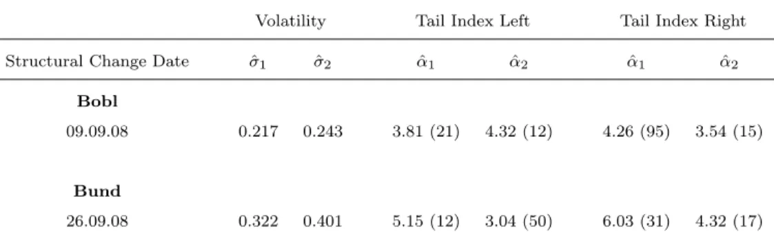
As response to the financial crisis in 2007/08 and the European sovereign debt crisis, the ECB started to conduct expansionary monetary policy on an unprecedented scale. In this paper I investigate the development of tail risks in the euro interest rate market since the implementation of this unconventional monetary policy. The focus of the study is on futures on German government bonds, namely the Bund, Bobl and Schatz, which are among the most relevant securities in this market. The analysis covers three aspects. First, I investigate if the daily returns of the futures exhibit fat tails over the period from 1999 to 2016 and if there are differences among these securities with respect to tail risk, as measured by the tail index. Second, I analyze if the tail risks are non-constant over the considered time period. Third, I study if the tail index contains information beyond the conventional risk measure volatility and its implications for value-at-risk considerations. Anticipating the results, this paper presents significant evidence for fat tails in the return distribution of the Bund, Bobl and Schatz future. In contrast to expectations, the results indicate the highest tail risk for the short-term Schatz future and the lowest for the long-term Bund future. Differences in market liquidity might be a reason for this. Furthermore, I find comprehensive evidence for an increase in right tail risk for all three futures around 2008. This increase is most significant for the long-term Bund future. Surprisingly, evidence for a decrease in left tail risk is found, although with lower significance. Additionally, the analysis reveals that tail index contains information, which is not captured by volatility. Thus, the results suggest that the accuracy of value-at-risk estimates for different long and short positions can be improved by taking into account the tail index explicitly in the estimation process.

(3)

List of Figures

1 Price Chart and Daily Future Returns over Time . . . 23

2 Recursive Tail Index and Test Statistic for the Bund Future . . . 32

3 Recursive Tail Index and Test Statistic for the Bobl Future . . . 33

4 Recursive Tail Index and Test Statistic for the Schatz Future . . . 34

5 Cumulative Distribution of Daily Bund Future Returns . . . 41

6 Rolling Daily Value-at-Risk Estimates at the 1% Critical Level . . . . 44

A.1 Hill Plots - Full Sample . . . 55

A.2 Hill Plots - First Sub-Sample . . . 56

A.3 Hill Plots - Second Sub-Sample . . . 57

A.4 Rolling Correlations of Daily Returns . . . 58

List of Tables

1 Descriptive Statistics of Daily Future Returns . . . 22

2 Sub-Sample Periods and Sizes . . . 25

3 Tail Index Estimates based on Exponential Regressions . . . 27

4 Results of the Recursive Test for Tail Index Constancy . . . 31

5 Comparison of the Tail Index and Daily Realized Volatility . . . 37

A.1 Tail Indices based on Hill Plots . . . 59

(5)

1 Introduction

Since the global financial crisis in 2008, risk management practices have become a major subject of debate in the financial industry. Due to the lack of regulation and proper risk management techniques prior to the crisis, global players like Lehman Brothers were able to perform highly questionable operations without estimating the underlying risk of these correctly. To make things worse, these risky operations were mainly financed with short-term funds, imposing further liquidity risk to the institution. After realizing severe losses due to the depreciation of mortgage-backed securities, rumours had spread in the market, questioning Lehman’s solvency and refinancing possibilities. Eventually this business model had to come to an end. On September 15th 2008 Lehman Broth-ers declared bankruptcy, remaining the largest bankruptcy filing in the history of the United States. Consequently, markets reacted heavily to this event and global stock indices realized significant losses. This date is known as the high point of the most severe financial crisis since the Great Depression in 1930. However, the case of Lehman Brothers was not the first nor the last extreme event during the course of the crisis.

Due to the interconnection of financial markets, the crisis spread globally. Many institutions had similar toxic assets on their balance sheets and even direct exposure to Lehman Brothers. Mistrust within the financial markets grew, which resulted in a stop of lending within the banking system. Important reference interest rates like Euribor and Libor started to increase significantly. Overnight the European interbank market froze, imposing liquidity shortages on large and systemically relevant banks. To pre-vent a collapse of the system, the ECB had to intervene with unconpre-ventional monetary policy measures and provide unlimited liquidity to the financial markets, given ade-quate collateral. Additionally, European governments had to structure immense rescue packages for troubled institutions, costing billions of tax payers’ money.

However, the economic consequences of this banking crisis remained fatal for many European countries. Not only were governments and the ECB challenged by economic contraction, but also by the European sovereign debt crisis, which persists until today. Especially peripheral countries like Portugal or Italy suffer from large amounts of public debt and household deficits relative to the size of their economies. Furthermore, the banking system in these countries is highly fragile, due to a large amount of non-performing loans and inadequately low capital buffers.1 _{The potential need of the banks}

for further public assistance intensifies the crisis and encounters incomprehension by

1

(6)

the citizens of these countries, who are confronted with poor economic conditions and reduced public benefits.

The heavy dependence of many European banks and even governments on the mas-sive liquidity supply of the ECB questions the long-term sustainability of the euro system as a whole. The current policy conduct of the ECB resulted in a low inter-est rate environment, which leads to a distortion of economic incentives and increased risk taking of market participants. Consequently, the actions of the ECB and related market factors are closely monitored by the public. Releases of economic data, rating agency decisions or ECB press conferences have become key events for the European financial markets. These events are usually accompanied by heavy price fluctuations, as market participants try to anticipate the outcomes. Therefore, the questions arise if the likelihood of so-called extreme events has significantly increased since the financial crisis in 2008 and if the participants in the financial markets are now exposed to higher market risks, despite all regulatory efforts in the recent past. This stresses the impor-tance of an accurate assessment and incorporation of extreme events in the market risk management of financial institutions.

Although great advancements in the assessment of extreme market events have been made since 2008, there is still large potential for further improvements and research in this area. Of special interest and significance is the euro interest rate market, which’s function was heavily disrupted during the financial crisis and is currently distorted by a low interest rate environment. The rates for transactions worth trillions of euros are determined in this market. Not only is it important for the financial industry itself but also for the overall euro economy, since credit conditions for housing or business investment depend on it through the reference rates Euribor and Eonia. Additionally, the refinancing costs of the majority of European states, of which some face currently enormous financial constraints, are determined in this market.

(7)

naturally to assume that there exist differences between the futures’ tail behavior, depending on the side of the distribution’s tail and the maturity of the underlying German government bond. The aim of this paper is to identify time and cross-sectional differences in the tail behavior of these euro interest rates futures. In general, there are three different standardized future contracts on German government bonds. These are the so-called Bund, Bobl and Schatz future, which have a long-term, medium-term, and short-term underlying bond maturity, respectively. Despite their differences in the underlying maturity and market liquidity, all three futures are used as the main hedging instruments for euro interest rate risk.

The tail behavior is worth studying for several reasons. First, it gives new insights into the occurrence of extreme euro market events and its implications for interest rate portfolios. Therefore, it allows financial institutions to assess market risks more accurately and contributes to the overall stability of the euro financial system, which has been immensely challenged since 2008. Second, the occurrence and severity of the financial crisis in 2008 question the underlying assumptions of many risk management techniques for trading activities. Of special relevance is the widely used assumption of a symmetric and normal return distribution, which underestimates the risk of extreme events and does not differentiate for long and short positions. Since activities of single trades have proven to lead to the failures of whole institutions in the past, the correct assessment of tail risk appears to be of great relevance in this context.2 _{Third, the}

identification of cross-sectional differences among the Bund, Bobl and Schatz future allows to the optimize hedging ratios of euro interest rate transactions, which implies not only more effective risk management but also cost reductions. Fourth, since the financial crisis in 2007/08 and the European sovereign debt crisis in 2010/11 the ECB has implemented many conventional and unconventional monetary policy measures, which resulted in a historical low interest rate environment. However, since this is a relatively new market environment, the effects of these policy measures are still not fully understood and require further investigation. As the ECB policy conduct aims, inter alia, at providing stability and reduce market uncertainty, its relation to tail risks in the euro interest rate market is of special interest and requires further research.

My analysis follows a similar approach to Werner and Upper (2002), who study the tail behavior of Bund future returns from 1997 to 2001. The focus is on the tail index

α, which measures the speed of the probability decay if one looks deeper into the tails of the return distribution. In general, a lower tail index implies thicker tails and thus,

2

(8)

higher tail risks, ceteris paribus. First, I analyze if the daily returns of Bund, Bobl and Schatz futures exhibit fat tails over the period from 1999 to 2016 and if there are significant differences among these three securities with respect to tail risk, as measured by the tail index α. Since the futures’ underlying bonds have different maturities and thus, durations, I hypothesize that the long-term Bund future realizes more extreme price fluctuations than the medium-term Bobl and short-term Schatz future. Therefore, the Bund future should also exhibit the highest tail risk, followed by the Bobl future and then the Schatz future.

Second, I investigate if the tail risk of the three future contracts has changed over the period from 1999 to 2016. Due to the massive market interventions by the ECB as response to the financial crisis and sovereign debt crisis, there has been an extreme change in the interest rate level in the euro zone. Therefore, I hypothesize a structural change in the tail indices around 2008, which represent an increase in the probability of extreme returns of the Bund, Bobl and Schatz future. In this case I anticipate that the Bund future is effected to the largest extend due to its highest underlying bond duration. Moreover, I expect that only the right tail of the return distributions indicates the higher probability of extreme returns, since the interest rate level in the euro zone primarily decreased since 2007 and did not rise considerably at any point in time. Due to the negative relation of interest rates and bond prices, extreme positive returns of futures on German government bonds should appear more often than negative ones since 2007.

Third, I analyze if the tail index contains further information beyond the conven-tional market risk measures volatility and its implication for value-at-risk estimates in case of euro interest rate futures. Since the concept of volatility refers to a sym-metric return distribution, the expected increase in the right tails’ fatness since 2008 might not be accurately assessed, which can lead to unexpected severe losses of short positions in the future contracts. Furthermore, several value-at-risk methods assume normality in the return distribution, which leads to a significant underestimation of tail events. Thus, I will also investigate the implications of this underestimation in terms of value-at-risk estimates.

(9)

long-term Bund future. Surprisingly, also evidence for a decrease in the left tail risks is found, although at lower significance. Furthermore, the analysis presented in this paper indicates that the tail index contains risk information, which is not captured by the concept of volatility. Consequently, the accuracy of value-at-risk estimates for different long and short positions in euro interest rate futures can be improved by taking into account the tail indexα explicitly in the estimation process.

The existing literature about the tail risks in the euro interest rate market is rather limited. Although, research about the tail-behavior of the long-term Bund future exists, it does not include the recent developments in the euro market. My analysis contributes to the existing literature in the following ways. First, to the best of my knowledge, I am the first one who investigates explicitly the tail behavior of the Bund, Bobl and Schatz futures since the financial crisis in 2008 and compares it to the situation before. Second, a comparison between these three futures contracts in terms of extreme risks over time has not been conducted before. Therefore, this analysis creates a basis for further research in the area of optimal hedging methods for euro interest rate transactions in the current market environment. Third, based on the contribution of Straetmans and Candelon (2013), I overcome a major shortcoming of the previous work by Werner and Upper (2002) in terms of over-rejection of tail index stability. Fourth, the present unconventional monetary policy of the ECB lacks of a comprehensive understanding of its market-wide effects. This analysis gives new insights in terms of tail risks in the euro interest rate market and the present monetary policy conduct. The results presented in this paper provide evidence for an increase in market risk in the current context of the expansionary monetary policy of the ECB, which represents an argument against its very extension.

(10)

2 Positioning in the Existing Literature

The distribution of financial returns has been a topic in academic research since decades, see Mandelbrot (1963) for an early analysis. Since this research area is not only the-oretical, but also highly relevant for many applications in the financial industry, the literature on return distributions has grown significantly over the years. Consequently, there are many papers covering not only stock returns but also other asset classes like fixed income, foreign exchange or commodities. Since the global financial crisis in 2008, a discussion about the appropriateness of risk management techniques of financial insti-tutions and their underlying assumptions has once again gained momentum. Of special relevance is the market risk management, which also comprises assumptions about the return distribution of financial assets. Here, the focus is on the tails of the distributions and the assessment of extreme events, which threaten the stability of whole financial systems.

Important research has been conducted in the area of extreme returns of bank stocks and the consequences for the stability of the banking system. However, the since 2008 produced literature on extreme events in the euro interest rate market is rather limited, despite its high relevance for the economic system. In case of the Bund, Bobl and Schatz future, this might be due to the lower perceived risk of the underlying bonds and their relatively low volatility. However, as Werner and Upper (2002) argue, this conclusion might be misleading considering the immense leverage in a future position on these bonds. This section highlights the need of more research in this area by giving an overview of the existing literature and analyzing its shortcomings, given the current market environment. Thereby, I position the paper in the current literature and explain its contribution to existing research. In the following I give an overview of the existing literature directly related to the Bund, Bobl and Schatz future. I also introduce conducted research concerning the tail behavior in other asset classes, since research specifically about the Bund, Bobl and Schatz future is limited and the underlying theory and methodology can be generally applied across all asset classes.

2.1 Tail Risk and the Bund, Bobl, and Schatz Future

(11)

in 2007/08, the European sovereign debt crisis in 2010/11 and the resulting monetary policy measures of the ECB, which lead to a historical low interest rate environment in the euro zone. This shortcoming will be addressed in my analysis, which uses a more recent sample period until August 2016. In their analysis Werner and Upper (2002) do not only use daily returns but also intra-day data, specifically, five minute returns and one hour returns. Thereby, differences in the tail behavior for different return frequencies are shown. However, since the future contracts are settled at the end of each trading day, the daily returns are of greater significance for risk management applications than the intra-day returns.

The authors find significant fat tails in the distribution of Bund future returns, which are not constant over time and change due to extreme events like the September 11th attacks. This result only applies to the higher frequencies of five minute and one hour returns and not daily returns. Over the considered time period, higher return frequencies appear to have fatter tails than lower frequencies. Moreover, the authors show that in case of the Bund future the tail behavior of a return distribution is not accurately captured by conventional market risk measures like volatility. Thus, the tail index α contains information, which is beyond standard risk measures.

In contrast, Werner and Upper (2002) do not investigate the tail behavior of the medium-term Bobl future and short-term Schatz future. Therefore, the cross-sectional differences between these securities are unidentified. Although the long-term Bund future has a significantly higher market liquidity, the Bobl and Schatz future are also frequently used for hedging interest rate transactions. This highlights the importance of a better understanding of the tail behavior of all three future contracts. In this paper I overcome this shortcoming and extend the analysis to the Bobl and Schatz future. In their methodology Werner and Upper (2002) use the Hill estimator to calculate the tail index for the Bund future return distribution. Since I apply this methodology in an identical version in my analysis, I explain this method in detail in Section 3 together with the shortcomings of the approach chosen by the two authors.

(12)

VaR, since the latter does not say anything about the actual loss. In this case especially the historical VaR estimates appears to underestimate the actual losses occurring. Us-ing the conditional VaR, the riskiness of the fund will be significantly reduced through decreasing the number of traded contracts by approximately twelve percent. Further-more, the author proposes to reduce the model risk in the Bund future’s VaR estimates by taking the highest estimate across all models. However, the study focuses only on the long-term Bund future and does not analyze the Bobl and Schatz future. Another shortcoming of the study is the outdated sample period, since it does not include the recent financial crisis and European sovereign debt crisis, which questioned the eff ec-tiveness of many risk management techniques. In this paper I address these two crises in VaR considerations for the Bund, Bobl and Schatz future.

In a more recent study Bessler and Wolff (2014) investigate how to optimally hedge European government bond portfolios during the sovereign debt crisis. For this a sample of daily observations is used, which ranges from January 2006 to December 2011. In contrast to previous literature, the authors do not only use the long-term Bund future but also the medium-term Bobl and short-term Schatz future as hedging instrument. Additionally, the BTP future on ten year Italian government debt is proposed as hedging instrument against the credit risk underlying European government bond portfolios. The concept of duration and the minimum variance approach are used to determine the optimal hedge ratio. Their study reveals that the Bund, Bobl and Schatz future were effective hedging instruments for EMU bond portfolios before the crisis and for government bonds with low credit risk during the crisis. Nevertheless, during the crisis the hedging effectiveness for EMU bond portfolios is significantly reduced if these three future contracts are used as single hedging instrument. In this case the Italian BTP future is a more effective single hedging instrument, since it also reflected the spike in credit spreads during the years 2010 and 2011, which was not the case for risk-free considered German government bonds. However, the main finding of the authors is that a joint hedge with German and Italian government bond future performs even better during the crisis compared to the single hedges. Bessler and Wolff (2014) conclude that a combination of the Bund, Bobl, Schatz and BTP future is the optimal hedging strategy to reduces the variance and also the tail risk of European government bond portfolios.

To the best of my knowledge, additional public available literature which covers explicitly the tail behavior of the Bund, Bobl and Schatz future does not exist. However, these three future contracts have been studied in a related topic by Fricke and Menkhoff

(13)

information share approach for the Bund, Bobl and Schatz future. Since the Bund future has the longest underlying bond maturity and highest market liquidity, one would expect that it dominates the two shorter maturity futures in terms of information shares. However, Fricke and Menkhoff (2011) show that the Bund future is indeed the most important contract in price discovery but does not dominate the two other contracts in each aspect. Instead, the medium-term Bobl and short-term Schatz future contain relevant information shares, which are occasionally even higher than the information share of the Bund future. This highlights the problematic of neglecting the less liquid Bobl and Schatz future. Thus, the findings by Fricke and Menkhoff (2011) provide a convincing argument that a comprehensive and complete market risk assessment should take into account all three future contracts.

The presented literature highlights two important aspects, which are not addressed by the analysis of Werner and Upper (2002). First, for applications in the industry it is essential to have a comprehensive risk assessment, which also includes the medium-term Bobl future and the short-medium-term Schatz future. Second, the recent financial crisis in 2007/08 has challenged many risk management models, which stresses the need of up-to-date research in this area. For a better understanding of the tail risk in the euro interest rate market, these two aspects are considered in the analysis presented in this paper. Additionally, to structurally underpin my topic on a fundamental level, I present in the following existing literature concerning the tail risk in other asset classes. Conveniently, the underlying theory and methodology is applicable to financial returns across all asset classes and thus, also relevant for my analysis.

2.2 Tail Risk and Other Asset Classes

(14)

downside risk and systemic risk. The considered time period starts in April 1992 and ends in June 2011, which includes the financial crisis and the European sovereign debt crisis. The left tail risk is used as indicator for the downside risk of banks’ stock returns and a tail-βis introduced as an indicator for systemic risk. Identical to my analysis, the tail risks are measured by the tail index α, which is estimated by the common method of Hill (1975). For a cross-Atlantic comparison of tail risks and systemic stability, banks in the euro zone and in the United States are considered. Their study reveals that the tail risk and systemic risk are higher for banks in the United States than for the euro zone regardless of the year. Furthermore, they find a significant increase in tail risk and systemic risk during the financial crisis. In contrast, the European sovereign debt crisis appears to have only a minor impact on banks’ equity capital. Similar to Straetmans and Chaudhry (2015), I investigate differences in market risk of euro interest rate futures during the financial crisis and sovereign debt crisis, since the crises underlying market mechanisms appear deviant.

Another study of the tail behavior in the asset class equity is provided by Lux (2001), who uses extreme value theory and intra-day data for the German stock index Dax 30 from 1988 to 1995. Similar to the other studies, the tail index estimation method by Hill (1975) is applied with several approaches to determine the optimal tail fraction in the return distribution. The analysis confirms previous studies and estimates a range for the tail index for the Dax index between three to four. Previous work by Müller et al. (1998), who use an alternative approach to define the extreme part in the tail of a return distribution, yields similar results. This confirms their findings robustness to the optimal choice of the tail fraction. Based on this approach, I apply in my analysis more than one method to determine the optimal sample fraction of extremes, which allows me confirm the robustness of my findings. Additionally, the study by Lux (2001) finds no evidence for an unstable tail behavior of Dax returns over the considered time period. These results are consistent even at lower data frequencies. In contrast, Jondeau and Rockinger (2003) look at several stock indices around the world and investigate differences in tail indices. Contrary to previous research, their results suggest no significant differences in the tail indices for the left and right tail of the return distribution. Moreover, their tail index estimates appear to be similar for the considered stock indices of different countries.

(15)

To determine the tail fatness the authors estimate the tail indexαbased on the method of Hill (1975). To test for the parameter stability, the tail index α is estimated over a pre-EMS period and EMS period. Identical to previous work, their results indicate significant fat tails for EMU exchange rate returns, which appear to be stable over time. In other words, this provides evidence that EMS did not lead to reduction of extreme exchange range volatility. Moreover, the study aims at identifying the most appropriate distribution assumption for these returns series. With estimated tail indices around the value two, their study contradicts previous work by Boothe and Glassman (1987), who estimate tail indices significantly above three and even find evidence related to a normal distribution. In later work Koedijk, Stork and de Vries (1992) study this subject in more detail. In my analysis I will follow a similar approach to Koedijk et al. (1990) and estimate the tail indexα over two sub-samples, one before the financial crisis 2008 and one after. However, in contrast to the authors, I will also apply a more formal test for structural changes in the tail index by Quintos et al. (2001) to confirm results in a more rigorous manner.

A multi-asset analysis of the tail risks over time is given by Straetmans and Candelon (2013). Their work constitutes an extension and refinement of the study by Quintos et al. (2001) and their previous paper Candelon and Straetmans (2006). In their empirical application the authors test for structural changes in the tail index for stock markets, bond market, currencies and commodities with a differentiation between developed and emerging markets. They show that stock market tails of emerging markets are not more prone to change over time than for developed countries. In contrast, this does not hold for currencies of emerging markets. The work by Straetmans and Candelon (2013) differs from the approach of Quintos et al. (2001) in two important aspects, which increase the accuracy and robustness of the findings. First, the optimal number of extremes in the tail is estimated through the minimum of the asymptotic mean squared error of the tail index, instead of using a fixed fraction of the extremes from the total sample. Second, the authors propose to use bootstrap-based critical values in tests for structural changes in the tail index. These take into account the bias in the estimates and solve the problem of over-rejecting the hypothesis of a stable tail index.

(16)

my analysis I also apply the structural change test by Quintos et al. (2001). However, I implement the augmented version of this test based on the proposals by Straetmans and Candelon (2013). In the following section the structural change test by Quintos et al. (2001) as well as the popular tail index estimation method by Hill (1975) are explained. Furthermore, I introduce several methods to estimate the optimal number of extremes in the tail, which allow me to confirm the robustness of my results.

3 Methodology

In order to test if there are difference in the tail behavior over time and between the Bund, Bobl and Schatz future, I will use the following approach. First, I present arguments for using a semi-parametric method. Second, I explain how I estimate the fatness of tails by the widely used concept of Hill (1975). Third, since the approach by Hill (1975) crucially depends on certain parameters, I will introduce several ways how to estimate these accurately. Fourth, in order to investigate if the tail risk of the euro interest rate futures has increased since 2008, I introduce the recursive test of Quintos et al. (2001), which allows to identify structural changes in the tail index. Since my analysis is based on the work by Werner and Upper (2002), I will use a similar methodology, which allows me to compare my results to the existing work in this field.

3.1 Fat Tails and the Hill Estimator

(17)

parametric models, one can use the empirical probability density function of financial returns. However, this requires a sufficiently large historical sample size, which is not always available. Consequently, due to the limit of historical samples, the analysis of extreme observations far in the tails might lack of accuracy and appears inappropriate for stability tests.

However, there exists an elegant way to combine the parametric and empirical ap-proaches and to overcome their individual limitations. This is the semi-parametric approach based on extreme value theory.3 _{Instead of making assumptions about the}

whole distribution range, the semi-parametric approach only assumes a certain distri-bution for the tails and uses the empirical probability density function for the remaining part. Huisman et al. (2001) argue that all fat tail distributions can be approximated by the Pareto distribution deep in the tails. Thus, I assume that the returns in the right tail of the three future contracts follow a Pareto-type distribution function:

1 F(x) = x−αL₍_x₎ α>0 (3.1)

In this case L₍_x₎ _{is a slowly varying function with} _lim

x→∞ L(λx)

L(x) = 1 for all λ > 0. The parameter α refers to the tail index and indicates the speed at which the mass in the tail decreases as one looks deeper into the tail. It is important to note that, keeping x constant, a lower tail index implies more mass in the tail, i.e. the probability of extreme returns is higher. In contrast, a higher tail index implies less probability mass in the tail and thus, lower tail risk, ceteris paribus. Mathematically the probability of extreme positive returns larger than x is given by P(X > x) = 1 F(x) = ¯F(x). Conveniently, the tail indexαalso indicates the existing number of moments. Therefore, a tail index smaller than four implies an infinitely high kurtosis. In contrast, under a normal distribution the tail index should in theory approach infinity.

Instead of aiming at a specification of the real parametric tail distribution of Bund, Bobl and Schatz future returns, I assume a Pareto-type distribution in the tails and estimate directly the tail index for each future contract. In general, a great advantage of this semi-parametric approach is that it allows to compare estimates based on different tail sizes. Since the aim of this analysis is to investigate the tail behavior, the negligence of information about the center of the distribution does not represent a disadvantage. There are several ways to estimate the tail index α of equation (3.1).4 _{However, I will}

3

A general analysis about extreme value theory and risk management methods is given Embrechts et al. (1999). For a more detailed discussion of the advantages and disadvantages of using extreme value theory for risk management purposes, see Diebold et al. (2000).

4

(18)

focus on the method introduced by Hill (1975), the so-called Hill estimator. Through its straightforward implementation, this method is widely used and serves as benchmark in many applications (Matthys and Beirlant, 2000). The Hill estimator is given by the following function:

ˆ

αHill = 1 ˆ γ =

1

k

X

i=1

lnxn−i+1 xn−k+1

!−1

(3.2)

with x1  x2 ... xn equal to the ascending order statistics of the empirical return

observations of the Bund, Bobl and Schatz future. In this form the Hill estimator is a maximum likelihood estimator for a Pareto-type distribution of the right tail. The parameter k in equation (3.2) refers to the number of extreme return observations considered in the tail. Therefore, assuming Pareto-type behavior in the tail of the return distribution, one only produces estimations about the area in the tail, which does not exceedk.

The described methodology of this semi-parametric approach refers to positive re-turns. However, I am interested in both sides of the return distribution. By estimating the tail index for each side of the distribution separately, I can differentiate the risk of extreme returns for different long and short positions in the future contracts. The expectation of different risks for long and short positions is supported by the fact that call and put options with same characteristics appear to have different implied volatil-ities.5 _{A convenient way to determine the tail index for the left side of the distribution}

with the Hill estimator (3.2) under the Pareto-type distribution assumption is simply to reverse the signs of the historical return series. The right tail describes then the actual negative returns and allows to reduce the computational burden for comparing the risk of long and short positions.

Despite its easy implementation, the Hill estimator has one significant drawback. Its estimates depend crucially on the number of extremes in the sample k. When choosing the optimal k, one is confronted with a trade-off. Increasing the number of extremes leads to a reduction in the estimator’s variance. However, at the same time, including more observations which are less “extreme”, also leads to an increased bias in the estimator. Consequently, the right choice ofk is an important part of this analysis and will be discussed in the following.

5

(19)

3.2 Determining the Optimal Number of Extremes in the Tail

The literature about determining optimal number of extremes k in the sample has grown significantly over the past decades.6 _{However, there is still no clear solution to}

this question. In order to verify the robustness of my tail index estimations, I will apply several approaches. First, I will apply the widely used method of Beirlant et al. (1999), which uses an exponential regression based estimator to quantify the variance-bias trade-off as a sample equivalent. As Straetmans and Candelon (2013) argue, the general principle underlying this method constitutes common practice in extreme value theory and thus, allows me to compare my results to previous work outlined in Section 2. Second, I will visualize this variance-bias trade-off through the conventional Hill plot, which allows me to confirm my previous results.

3.2.1 Estimates based on the Exponential Regression Model

The idea of the algorithm by Beirlant et al. (1999) is to quantify the variance-bias trade-offthrough the asymptotic mean squared error of the Hill estimator and choosing its minimum.7 _{For this Beirlant et al. (1999) derive the following exponential regression}

model for the log spacing of the order statistics:

j(log xn−j+1,n log xn−j,n)⇠ γ+bn,k

✓ j k+ 1

◆−ρ!

·_f_j ₁__j __k _(3.3)

where bn,k is equal to b n_k₊₁+1 with 1  k  n 1. Moreover, (f1, f2, ...fk) is a vector

of independent standard exponential random variables. In this case the inverse of the Hill estimator (3.2) represents a maximum likelihood estimator for γ in the following simplified model:

j(log xn−j+1,n log xn−j,n)⇠γ·fj 1j k (3.4)

It can be shown that the Hill estimator is asymptotically normal when k grows at a sufficiently lower rate thann, so that the ratio k

n converges to zero in infinity. Beirlant

et al. (1999) argue that the bias in model (3.4) arises through excluding the regression

6

For an overview of the main types of adaptive threshold selection methods, see Matthys and Beirlant (2000).

7

(20)

terms of the full model (3.3). The authors show that this bias can be approximated by:

Bias(αHill k,n )⇠

bn,k

1 ρ

Additionally, the variance of the Hill estimator is approximated by:

V ar(αHillk,n )⇠ α2

k (3.5)

Thus, the variance-bias trade-off can be calculated as the asymptotic mean squared error of the Hill estimator:

AM SE(ˆα_k,nHill) =AV ar(ˆα_k,nHill) +ABias2(ˆαHill_k,n ) = γkˆ

2

k +

ˆ_b_n,k 1 ρˆk

!2

(3.6)

From this the estimator for the optimal number of extremes in the tailˆkcan be identified as the point where the asymptotic mean squared error of the Hill estimator reaches its minimum:

ˆ

k_n,opt₂ =argmin 3≤k≤n

0

@

ˆ γ2

k +

ˆ_b_n,k

1 ρˆ

!21

A

In order to determine the optimal fraction of extremes in the distributions of the Bund, Bobl and Schatz future returns, I estimate the exponential regression model (3.3) and determineγkˆ andˆbn,k with3k 500for each tail side of three future contracts.8

Identical to Matthys and Beirlant (2000), I do not estimate ρ, but fix the value at -1 throughout my analysis. The authors argue that for many distribution fixing this parameter performs better, with respect to the MSE, than estimating it, even if specified inaccurately. This also corresponds to the findings of Drees and Kaufmann (1998). With the resulting estimatesˆγk andˆbn,k I calculate the asymptotic mean squared error

of the Hill estimator with equation (3.6) for each k. Based on the minimum of the AM SE(ˆα_k,nHill), I get an estimate for the optimal sample fraction of extremesk for each tail side of the distributions. With these ˆkn,opt2 I calculate the tail index for the daily return distributions of the Bund, Bobl and Schatz future according to the Hill estimator (3.2).

8

I reduce the computational burden and do not estimate model (3.3) fork 500_{. Given the total}

(21)

3.2.2 The Hill Plot

Additional to the quantitative approach of Beirlant et al. (1999), I produce Hill plots for each future’s tail side. This allows me to visualize the variance-bias trade-off and to confirm my results from the previous method. The Hill plot is a simple and effective method to determine the optimal number of extremes through the so-called “Eye-Balling technique”. The Hill estimates are plotted for all possible values of k in an ascending order. The optimal number of extremes is then estimated visually in the area where the variance of Hill estimator is sufficiently low i.e. whereαˆ appears stable to the choice of k and the bias is not too large.

The major disadvantage of this heuristic method is that the results are subjective and not based on quantitative analysis. Consequently, an exact determination of the optimal number of extremes is difficult and the results might be inaccurate. Since the Hill estimator is highly sensitive to the choice of k, there is significant potential for estimation errors. However, I will use the estimates of Hill plot only as a supportive argument to verify the results from the Beirlant et al. (1999) method.

In contrast, Werner and Upper (2002) do not use the Hill plot to verify their results but the regression approach of Huisman et al. (2001). Their method uses a weighted average of a set of Hill estimates, each based on a different number of extremes in the tail. The weights are determined through OLS estimation. In this approach the number of extremes is a constant fraction of the sample size κ = k

n. However, Straetmans

and Candelon (2013) and Dumouchel (1983) argue that under this assumption the Hill estimator lacks of asymptotic normality, since the number of extremes does not increase at a sufficiently low rate as the overall sample size grows. Therefore, I will not use the method of Huisman et al. (2001) to verity the results of the other methods. Nevertheless, for sake of completeness and comparability to Werner and Upper (2002), I report tail index estimates based on the Huisman et al. (2001) method in the appendix.9

3.3 Identifying Structural Changes in the Tail Behavior

In order to investigate if the tail behavior of the Bund, Bobl and Schatz futures changed during the financial crisis and sovereign debt crisis, I apply the method by Quintos, Fan and Phillips (2001). In their analysis the authors use three different tests to identify structural changes in the tail behavior, which are the recursive, sequential and rolling test. Each of them is based on a different division method of sub-samples for the Hill

9

(22)

estimator. However, in simulations Quintos et al. (2001) show that the recursive test dominates in identifying change dates and in finite sample power. Consequently, I will only apply the recursive test, which’s statistic is calculated according to the following:

Y_n2(r) =

✓ t⇥kt

n ◆ ✓

ˆ αt ˆ αn 1

◆2

(3.7)

withr= t

n as in increasing fraction of the full sample and αnˆ equal to the Hill estimate

for full sample n. The sample size r is increased successively by one daily observation. The recursive version of the Hill estimator (3.2) is defined as:

ˆ αt=

1 ˆ γt

= 1

kt kt−1 X

i=0 ln

✓ xt−i,t

xt−k,t

◆!−1

(3.8)

In order to estimate kt I follow the approach by Straetmans and Candelon (2013). In

this case,kˆt = ˆct

2

3 with ˆc= ˆkn

n23 as the full sample scaling constant. This ensures that

ˆ

k grows at a sufficiently low rate as n increases. In my analysis I calculateˆcfor each tail side of the Bund, Bobl and Schatz future. I determine the optimal number of extremes in the full samples ˆkn according to the algorithm by Beirlant et al. (1999).

The hypothesis of a constant tail behavior of euro interest rate futures over time can be formally expressed as:

H0 :α[t]=α HA:α[t]6=α

The null hypothesis of constancy is most likely to be rejected at the time where the estimated recursive test statistic reaches its supremum:

Q= sup

r∈Rτ

Y_n2(t)

(23)

the bias in the Hill estimator.

As proposed by the two authors, I use bootstrapped-based critical values at the 95% and 99% confidence level. To determine these, I estimate a GARCH(1,1) model for the Bund, Bobl and Schatz return series, respectively. From this I extract the estimated daily volatilities. To create 10,000 return sample replications for each of the three futures, I multiply the extracted daily volatiles with by random variables which follow

N₍₀_,₁₎_{. The results are 10,000 replicated samples of 4489 daily return observations}

for each of the three future contracts. I use these sample replications to calculate the simulated recursive test statistics by the described methodology of Quintos et al. (2001). From the resulting simulated distribution of bootstrap-based recursive test statistics, I use the 1% and 5% quantiles as my critical values, respectively. Since I use different values forˆknfor each tail side in the estimation of the recursive Hill estimator (3.8), the

bias will be different for each tail side. Thus, I determine separate critical values for the left and right tails of the three futures’ return distributions. This results in twelve bootstrap-based critical values for the 95% and 99% confidence level.

Since there were significant changes in monetary policy during the financial crisis, I expect the supremum of the recursive test statisticsQ to occur during the years 2008 or 2009. Furthermore, since I cannot exclude the possibility of a decreases in the tail risks for Bund, Bobl and Schatz future, I perform also a backward version of the recur-sive test, as implemented by Straetmans and Candelon (2006, 2013). For this I simply revert the sample, with the latest observation being the first, and re-estimate the recur-sive test statistics (3.7) and Hill estimates (3.8). While the regular “forward recurrecur-sive test” signals decreases in the tail index, the “backward” version indicates increases in the tail index. In the following section I describe in detail the data series I use for these test.

4 Data Series

(24)

securities are Italian and Spanish government bonds, respectively. Since the aim of this analysis is, inter alia, to investigate cross-sectional differences among the Euro Bund, Bobl and Schatz future, it is important to differentiate precisely the underlying bonds of these futures, as done in the following.

4.1 The Bund, Bobl and Schatz Future

In general, within future contracts there has to be a differentiation between contract size and price. The contract size refers to the deliverable quantity of the underlying asset. In case of one Bund, Bobl and Schatz future this is equal to EUR 100,000 of German government bonds with the respective maturity.10 _{The prices of these futures}

are quoted as percent of the par value. For instance, a quotation of 150.00 for one future refers to a price of EUR 150,000 for EUR 100,000 face value plus coupons of a German government bond with the respective maturity. Consequently, the tick value of this future is EUR 10.

Specifically, the long-term Euro Bund (Bundesanleihe) future has an underlying German government bond with a remaining maturity of ten years and a coupon rate of 6%. However, since on delivery day there is not always a bond with these characteristics available in the market, the underlying bond is actually fictitious. Alternatively, the short position in the future contract can deliver a German government bond, which is equivalent to the one specified in the future. In case of the Bund future, deliverable eli-gible bonds have a remaining maturity between 8.5 and 10.5 years, an original maturity of no longer than 11 years and minimum issue amount of EUR 5 billion. Based on the so-called conversion factor, the delivered amount of the eligible bond is adjusted in such a way that it matches value of the fictitious bond underlying the future. Since there are usually several eligible bonds, the short position will always choose the one which is the cheapest to deliver. Furthermore, it is important to know that the long-term Bund future is widely used as an indicator about the future interest rates levels in the euro zone. Due to the negative relation between bond prices and interest rates, a price increase in the Bund future indicates market expectations about falling interest rates, while a price decrease signals a rise in interest rates.

In case of the medium-term Euro Bobl (Bundesobligation) future the underlying German government bond has maturity of five years and a coupon rate of 6%. Again, on delivery date this underlying bond is rarely available in the market and therefore,

10

(25)

actually fictitious. In this case alternative eligible German government bonds for deliv-ery must have a remaining maturity of 4.5 to 5.5 years. The short-term Euro Schatz (Bundesschatzbrief) future has an underlying German government bond maturity of two years with a coupon rate of 6%. Here, for delivery eligible German government bonds must have a remaining maturity of 1.75 to 2.25 years.

In general, the three interest rate futures have expirations up to nine months and expire in March, June, September and December of each year. Depending on the expiration date there are price differences in the futures. For my analysis I will only look at the most actively traded contract, which is generally the one with the nearest expiration date. This future is rolled over on the last Thursday of the trading period. The last trading day is two exchange days prior to the delivery day of the relevant contract. Conveniently, Bloomberg offers adjusted time series price data, which links all most active contracts over a desired time period. Additionally, it should be noted that there is also Euro Buxl (Bundesanleihen extra large) future, where the underlying fictitious German government bond has a maturity of 30 years and a coupon rate of 6%. Nevertheless, since this contract is significantly less traded in the market and hardly used for hedging purposes, I will not include it in the analysis and only focus on the three main futures Bund, Bobl and Schatz.

4.2 Retrieving and Transforming the Data

In order to investigate the tail behavior of euro interest rate futures, I retrieve daily clos-ing price data for the most active Euro Bund, Bobl and Schatz futures from Bloomberg, which is already adjusted for rollovers. The time period for my analysis starts January 4th 1999 and ends on August 22nd 2016. This implies a total sample size of 4490 daily price observation for each future. From these I calculate the daily logarithmic returns byrt=ln

⇣

P ricet

P ricet−1

⌘

. Using the natural logarithm of returns has the advantage of time-additivity. Moreover, for all three future contracts the returns satisfyrt⌧1, implying

approximate equality of log and raw returns. The presented calculations and figures in this paper have been produced in MATLAB R2015b and Microsoft Excel 365.

(26)

Bund Bobl Schatz Bund Bobl Schatz Bund Bobl Schatz

01/1999 - 08/2016 01/1999 - 07/2008 08/2008 - 08/2016

Mean Return 0.008 0.005 0.001 -0.001 -0.001 -0.001 0.019 0.011 0.004

Max Return 1.959 1.238 0.577 1.271 0.956 0.577 1.959 1.238 0.527

Min Return -2.267 -1.722 -0.737 -1.490 -1.197 -0.737 -2.267 -1.722 -0.612

Volatility* 0.359 0.229 0.088 0.320 0.216 0.095 0.401 0.243 0.078

Kurtosis 5.50 9.42 10.37 4.29 5.61 8.45 5.73 12.14 14.05

Skewness -0.40 -0.94 -0.69 -0.41 -0.64 -0.74 -0.42 -1.20 -0.51

Mean Volume** 798 453 396 877 470 417 705 433 372

Notes: The presented figures are based on daily frequency. The returns are calculated as log returns and presented as percentage.

*Refers to the daily standard deviation of returns as percentage.

**The mean volume refers to the average daily trading volume in thousands.

Table 1: Descriptive Statistics of Daily Future Returns

future and the smallest for the Schatz future. This indicates that, in terms of market risk, a position in the Bund future has historically the highest risk. However, from the volatility the risk of a short and long position cannot be differentiated and therefore, can lead to wrong conclusions. Moreover, the kurtosis value of all three futures is clearly above the normal distribution value of three, which implies fat tails. Surprisingly, the short-term Schatz future has the highest kurtosis value and the long-term Bund future the lowest value. This can be seen as a first indication for cross-sectional differences in the tails of the return distribution between the Bund, Bobl and Schatz future.

Nevertheless, it should be noted that there are several drawbacks in using the kur-tosis as a measure of the tail heaviness. As Brys, Hubert and Struyf (2006) argue, there is no general agreement on what kurtosis actually estimates, since it is also used to measure the peakedness of a distribution. Analogously to the volatility, the kurtosis value also does not allow to differentiate the fatness of the left tail and right tail of the return distributions. Due to its restriction to symmetric distributions, the fourth moment is an inappropriate market risk measure of extreme events for different long and short positions. This stresses the importance of a detailed analysis, which considers the tails of the return distributions separately, as performed in this paper.

(27)

-2.25% -1.75% -1.25% -0.75% -0.25% 0.25% 0.75% 1.25% 1.75%

1999 2001 2003 2005 2007 2009 2011 2013 2015

Re

tu

rn

Bund 100

110 120 130 140 150 160 170

1999 2001 2003 2005 2007 2009 2011 2013 2015

C

o

n

tr

ac

t

V

al

u

e

Bund Bobl Schatz

-1.75% -1.25% -0.75% -0.25% 0.25% 0.75% 1.25%

1999 2001 2003 2005 2007 2009 2011 2013 2015

Re

tu

rn

Bobl

-0.75% -0.50% -0.25% 0.00% 0.25% 0.50% 0.75%

1999 2001 2003 2005 2007 2009 2011 2013 2015

Re

tu

rn

Schatz

Notes: The contract value of the three futures in the upper part of the figure is shown in thousands of euros.

(28)

is significantly more traded than the Bobl and Schatz future and therefore, has the highest market liquidity.

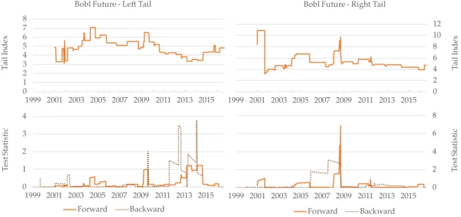
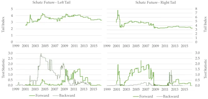
In order to analyze the price development over time, Figure 1 shows the price chart and the daily returns of the three futures over the whole sample period. Usually, due to the longest underlying bond maturity, the Bund future has the highest price. Since the middle of 2008, the contract prices of all three futures rose, especially of the long-term Bund future.11 _{Moreover, from the three lower graphs in Figure 1 it appears that the}

number of extreme returns has increased since 2008 for all three future contracts. It seems that this increase has been persistent until today, except for the Schatz future. Additionally, there has been relatively high volatility and also clustering for all three futures around the financial crisis in 2008 and the European sovereign debt crisis in 2011. In case of the Bund future the volatility is also clustered in the beginning of 2015, when the ECB implemented its quantitative easing program.

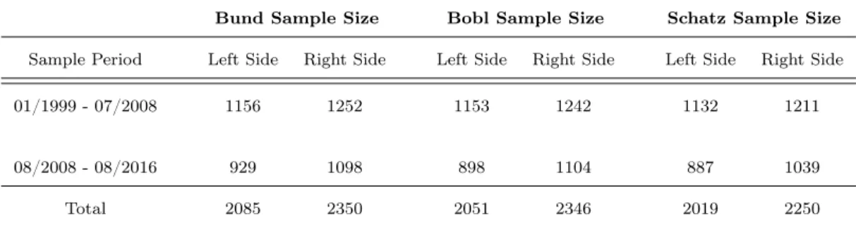
Since the purpose of this analysis is, inter alia, to study the time variation the tail behavior of euro interest rate futures, I follow the approach by Koedijk, Schafgans and de Vries (1990) and create two sub-samples. The first sub-sample only contains the returns prior to the collapse of Lehman Brothers and the resulting interventions by the ECB. Since the ECB already indicated in late August 2008 to lower the key interest rates, I define the first sub-sample period from January 1991 to July 2008. The second sub-sample period is from August 2008 to August 2016 and contains all returns following the financial crisis, the European sovereign debt crisis and all related monetary policy measures. Table 2 shows the resulting sub-sample sizes for each future and the respective return distribution side.12 _{Each tail side of the respective future contract}

and sub-sample has roughly 1000 observations. The first sub-sample is slightly larger than the second sample, due to an additional year of consideration. However, using the methodology described in Section 3, the outcome of the empirical study should not be effected by this minor difference, as long as the number of extremesk in the tails grows at an appropriate low rate with the sample size n (Diebold et al., 2000).

The middle and right part of Table 1 show the descriptive statistics for the first sub-sample and the second sub-sample, respectively. There are significant differences in all statistics over the two sub-periods. Before August 2008 all three futures have a negative mean return of 0.001%, while after this date the daily mean returns are significantly positive, especially for the Bund future with 0.019%. Moreover, regarding

11

On June 14th 2016 the price of the Euro Bund future reached for the first time more than 165.00, implying a negative yield on a ten-year German government bond.

12

(29)

Bund Sample Size Bobl Sample Size Schatz Sample Size

Sample Period Left Side Right Side Left Side Right Side Left Side Right Side

01/1999 - 07/2008 1156 1252 1153 1242 1132 1211

08/2008 - 08/2016 929 1098 898 1104 887 1039

Total 2085 2350 2051 2346 2019 2250

Notes: The sample sizes refer to daily observations.

Table 2: Sub-Sample Periods and Sizes

extreme returns, the maximum and minimum returns of the full sample occurred after July 2008, except for the Schatz future. Similarly, in case of the Bund and Bobl future, the volatility indicates a larger range of price fluctuations in the second sample. In contrast, the short-term Schatz future has a higher daily volatility before August 2008. The kurtosis value for all futures increases in the second sample, which indicates even more probability mass in the tails, compared to the normal distribution. As before, the Schatz future has the highest kurtosis value, followed by the Bobl future. Similarly, the return distributions of the Bund and Bobl future are more negatively skewed in the second period, although only marginally in case of the long-term Bund future. However, the short-term Schatz future is less negatively skewed in the second period. Together with the higher kurtosis values, this represents a first sign of variation in the tail behavior over time for all three future contracts, which is investigated further. Additionally, the average daily trading volume is lower in the second sample period for all contracts, but especially for the Bund future. This might be due to tighter market regulations introduced since the financial crisis.

(30)

5 Empirical Results for the Tail Behavior

I want to investigate whether the tail risk of euro interest rate futures has increased since the financial crisis in 2008 and the resulting loose monetary policy of the ECB. Moreover, I would like to identify if there are differences in the tail risks between the Bund, Bobl and Schatz future. First, I will present the Hill estimates for each future contract over two different sub-sample periods. Second, I will show the results of the recursive test by Quintos et al. (2001) to identify potential change dates and thereby, verify the differences in the Hill estimates from the previous part.

5.1 Comparing Tail Index Estimates

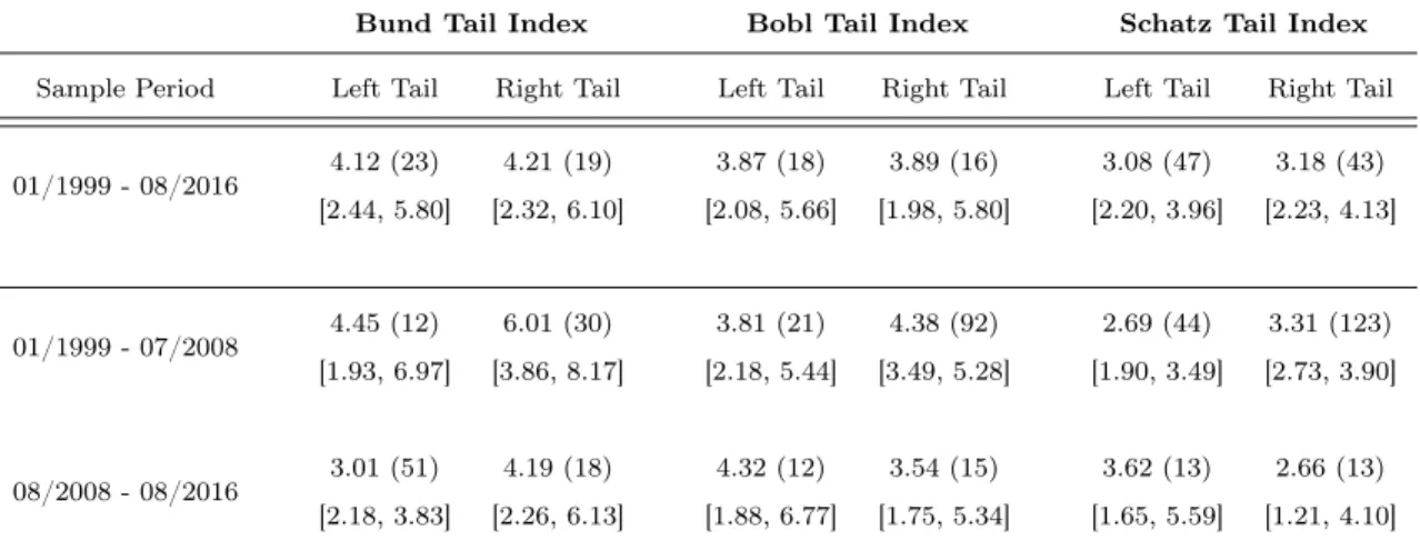
Table 3 shows the Hill estimates based on equation (3.2) for the tail indices of the Bund, Bobl and Schatz future returns. Here, I differentiate between the left tail and right tail to determine the risk of long and short position in the futures separately. Moreover, Table 3 presents Hill estimates over three different sample periods. The full sample uses the data range from January 1999 to August 2016. The first sub-sample is based on returns from January 1999 until July 2008. The second sub-sample only contains information from August 2008 to August 2016. The optimal sample fractions of extremes are based on the algorithm of Beirlant et al. (1999) and presented for each sub-sample in round brackets behind the estimates. Moreover, Table 3 shows the 95% confidence intervals for the Hill estimates below each estimate in square brackets. Given the approximation for the variance of the Hill estimator in equation (3.5) on page 16, I calculate the confidence intervals by:

CI(ˆα) = ˆα±_z αˆ

p

ˆ

k

(5.1)

(31)

Bund Tail Index Bobl Tail Index Schatz Tail Index

Sample Period Left Tail Right Tail Left Tail Right Tail Left Tail Right Tail

01/1999 - 08/2016 4.12 (23) 4.21 (19) 3.87 (18) 3.89 (16) 3.08 (47) 3.18 (43) [2.44, 5.80] [2.32, 6.10] [2.08, 5.66] [1.98, 5.80] [2.20, 3.96] [2.23, 4.13]

01/1999 - 07/2008 4.45 (12) 6.01 (30) 3.81 (21) 4.38 (92) 2.69 (44) 3.31 (123) [1.93, 6.97] [3.86, 8.17] [2.18, 5.44] [3.49, 5.28] [1.90, 3.49] [2.73, 3.90]

08/2008 - 08/2016 3.01 (51) 4.19 (18) 4.32 (12) 3.54 (15) 3.62 (13) 2.66 (13) [2.18, 3.83] [2.26, 6.13] [1.88, 6.77] [1.75, 5.34] [1.65, 5.59] [1.21, 4.10]

Notes: The presented tail index values are based on the minimumAM SE( ˆα) estimated through the algorithm by Beirlant et al. (1999) for each respective sub-sample. The corresponding optimal number of extremesk is shown in round brackets behind each estimate. The square brackets below each estimate indicate their 95% confidence interval.

Table 3: Tail Index Estimates based on Exponential Regressions

tends to be smaller than the left tail indices. This matches the analysis of Werner and Upper (2002) and the empirical fact, that market downturns are usually more extreme in magnitude than market booms. Consequently, the market risk of long position in these future contracts appears to be higher than of a short position.

Considering now the tail index estimates over the two individual sub-samples. In case of the Bund future, the estimate for the left tail decreases from 4.45 to 3.01 and also for the right tail from 6.01 to 4.19. The upper bound of the confidence interval indicates an unbounded fourth moment for the left tail after July 2008. Although the confidence intervals for the two periods are overlapping, the decrease in the upper bounds in the second period and the smaller confidence interval suggest a decline in the tail indices. These tail index estimates are consistent with the values of Herlemont (2005), who identifies a tail index range from three to six for daily Bund future returns from 1990 to 2004. Thus, the presented estimates indicate that the risk of extreme returns has increased since 2008. In other words, the tail risk for long position in the Bund future is higher than for a short position before and after 2008.

(32)

3.31 to 2.66 for the right tail. Before August 2008 the upper bounds of the confidence intervals for the left and right tail are smaller than four, indicating an unbounded fourth moment for the Schatz future during this period.

Despite for the left tail of the Bund future, the indicated development of the tail index estimates and confidence intervals is in line with the expectations based on the current monetary policy conduct. The since August 2008 implemented measures by the ECB aimed at lowering the interest rate level in the euro zone, including long-term rates, which are relevant for business investment. Consequently, the prices of German government bonds rose significantly and realized more often large positive returns than negative returns, as visualized by the price chart in Figure 1 on page 23. The increase in probability mass in the right side of the return distributions since mid 2008 is indicated by the lower estimated tail indices for all three futures.

A possible explanation for the indicated rise in left tail risk for the Bund future is the expected length of the business cycle. The Bund future price is based on the long-term yield curve up to 10.5 years. Based on past economic crises and market expectations, this time frame does not only comprise recessions but also the following economic boom, which is usually accompanied by higher inflation and a tightening of monetary policy. Therefore, at the time of introducing loose monetary policy, the expected reversal from this policy over the following five to ten years can lead to a higher expected probability of extreme negative returns in the Bund future. Since the underlying bonds of the Bobl and Schatz future do not cover the part of the yield curve beyond 2.25 and 5.5 years, respectively, their prices might not reflect the possibility of a tightening of monetary policy after this period. Thus, the risk of extreme negative returns is lower for these bonds, as indicated by the increased left tail index estimates for the Bobl and Schatz future in the second period. However, it is important to note that, despite the decreased upper bounds, the overlap of confidence intervals over time stress the need for further study in a more formal manner, as implemented in the next section.

(33)

sensitivity to changes in the yield curve and thus, a higher potential for large price changes. However, the estimates for the indices point out the reverse pattern. As in the comparison over time, the overlapping confidence intervals highlight the importance of further tests to confirm these cross-sectional differences.

A possible explanation for this ranking of tail risks might be differences in market liquidity of the futures. Looking at the descriptive statistics in Table 1 on page 22, one can see that the daily average trading volume of the Bobl future is almost half compared to the Bund future and even lower for the Schatz future.13 _{The lower market}

liquidity implies a higher chance for market participants to influence prices by “cornering the market”.14 _{Consequently, the price of the short-term Schatz future might be more}

sensitive to large trading orders compared to the medium-term Bobl future and the highly liquid Bund future. The resulting potential for large significant price drivers might explain the fatter tails for the shorter underlying bond maturities. However, to prove the potential for market cornering in the short-term euro interest rate market, further empirical investigation is required.

It is important to note that the results presented in this analysis are solely based on the method of Beirlant et al. (1999), which induces model risk to the presented estimates. Moreover, since the confidence intervals of the tail index estimates are often overlapping in time and cross-sectional comparisons, the accuracy of presented tail index differences is significantly limited. Therefore, in order to reduce the model risk and to confirm the robustness of the presented indications, I also estimate the tail indices based on Hill plots. The results are presented in Table A.1 on page 59 in the appendix. Moreover, Figure A.1, A.2 and A.3 in the appendix show the Hill plots for the Bund, Bobl and Schatz future over the three different sample periods. For the sake of comparison to Werner and Upper (2002) and despite the mentioned shortcomings, I also report the tail index estimates based on the method of Huisman et al. (2001) in Table A.2 in the appendix. Although the estimates of the two alternative methods differ slightly in magnitude, the general indications and conclusion confirm the estimates from the Beirlant et al. (1999) algorithm. Once more, the short-term Schatz future appears to have the highest tail risks, while the long-term Bund future the lowest. Therefore, the results presented in this section, provide some first indications for time and cross-sectional differences in the tail behavior of euro interest rate future returns. However, from this it is not clarified when exactly the tail risks of the future contracts changed.

13

From January 1999 to August 2016, the daily trading volume of the Schatz future was on 264 days less than 20% of the Bund future trading volume.

14

(34)

To proof the differences over time in a more rigorous manner, I will apply the structural change test by Quintos et al. (2001) in the following section together with the proposed augmentation by Straetmans and Candelon (2013).

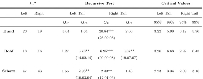
5.2 Testing for Structural Changes in the Tail Behavior

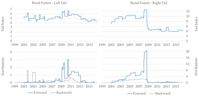
The results in the previous analysis give a first indication of time variation in the tail behavior of euro interest rate futures. In order to investigate these structural changes more formally and to identify potential change dates, I apply the recursive structural change test by Quintos et al. (2001), as introduced in the methodology Section 3.3. The results of the tests for the Bund, Bobl and Schatz future are presented in Table 4. The recursive test starts with a sample size of 500 observations and is increased successively by one daily observation. The supremum of the statistic for the forward version of the testQF indicates decreases in the tail index, while the supremum of test statistics for the

backward versionQBindicates increases in the tail index. The results are differentiated

for each tail side. The optimal number of extremes in the samplek is estimated through the method by Beirlant et al. (1999) and used for the estimation of the test statistics and the bootstrap-based critical values. As shown by Straetmans and Candelon (2013), the bootstrap-based critical values apply for the forward and backward version of the recursive test. Since the bootstrapped-based critical values take into account the bias in the Hill estimator, the presented numbers in Table 4 are greater than the asymptotic critical values of 1.78 and 2.54 used by Quintos et al. (2001) and Werner and Upper (2002). This solves the problem of an over-rejection of the constant tail index null hypothesis. Moreover, the recursive test statistics of equation (3.7) and the recursive tail index estimates of equation (3.8) for the Bund, Bobl and Schatz future are plotted in Figure 2, 3 and 4, respectively. Since the recursive test starts with 500 observations, the estimates for first two years 1999 and 2000 are lost.