Estud. Econ. vol.42 número1

(1)

Est. Econ., São Paulo, vol. 42, n.1, p. 43-74, jan.-mar. 2012

ISSN 0101-4161

Residual and Technical Tax Eficiency Scores for

Brazilian Municipalities:

a Two-Stage Approach

Maria da Conceição Sampaio de Sousa

Professora do Departamento de Economia, Universidade de Brasília (UnB) - Campus Darcy Ribeiro Universidade de Brasília - Caixa Postal 4320, CEP: 70910-900, Brasília - DF.

E-mail: csampaiodesousa@gmail.com

Pedro Lucas da Cruz Pereira Araújo

Doutorando em Economia, Universidade de Brasília (UnB) - Campus Darcy Ribeiro Universidade de Brasília - DF - Caixa Postal: 4320 - CEP: 70910-900

E-mail: araujo.pedrolucas@gmail.com

Maria Eduarda Tannuri-Pianto

Professora do Departamento de Economia, Universidade de Brasília (UnB) - Campus Darcy Ribeiro, Universidade de Brasília, Caixa Postal, 4320 - CEP: 70910-900 - Brasília - DF.

E-mail: maria.tannuri@gmail.com

Recebido em 05 de março de 2010. Aceito em 25 de outubro de 2011.

1. Introduction

Recurrent fiscal imbalances in terms of tax and expenditure assign-ments among central and local governassign-ments are a critical issue in public finance. To equalize tax capacities, cope with spillovers or to achieve national policy objectives, central governments often provide transfers to lower levels of government. These transfers may affect the incentives to improve fiscal performance because they may induce low tax effort in the regions (Litvack, Ahmad and Bird, 1998; Boadway

et al., 1999).

This point is particularly relevant for Brazil, as the Constitution of 1988 assured a substantial financial autonomy for subnational governments by increasing the share of public resources accruing to states and municipalities. However, this revenue decentraliza-tion was not followed by a decentralizadecentraliza-tion of responsibilities as no conditions were imposed concerning the use of the shared revenues.

Concerning this “incomplete ﬁscal decentralization”, where spending

(2)

44_{Maria da C. S. de Sousa, Pedro Lucas da C. Araújo e Maria Tannuri-Pianto}

on transfers from the central government, two points deserve to be noticed. Firstly, the lack of tax capacity and managerial abilities for most of the municipalities and secondly, inflated municipalities’ ex-penditures to match their increasing revenues. Additionally, the pro-liferation of small cities without any fiscal viability and no reliable human resources led to significant imbalances that were transferred to the federal level (Rezende, 1995; Varsano and Mora, 2001).

To cope with the deterioration of municipal finances, a complex system of federal and state transfers set apart expenditure deci-sions from tax capacity in local jurisdictions as the provision of local public goods rely heavily on those transfers. In this scenario, the

reduced productivity of local tax bases can be partly explainedby

their low tax effort, since it isless costly to obtain resources through

transfers from otherspheres of government than to exploit their own

taxbase. Even a greater reliance on property taxes has not

increa-sed the much required degree offiscal autonomy at the local level.

However, this dissociation between municipalities’ financing needs and their revenues cannot go on indefinitely.

The upsurge of municipal expenses, brought about by the decentra-lization of public spending granted by the 1988 Constitution and a higher urbanization, together with the fiscal strain faced by the higher levels of government threaten the perpetuation of the current model. For that reason, in recent years, there is an increasing empha-sis on the necessity to increase municipalities’ tax capacity and the efficiency of tax collection. Hence, tax efficiency measurements are relevant for implementing a sound tax system.

Traditionally, tax effort is computed as a ratio between the obser-ved tax collection and its potential, where the latter comes from

regression analysis or stochastic frontiers (Blanco, 1998; Baretti et

al., 2000; Jha et al., 1999; Bahl, 1971). As an alternative to this

approach, a few studies used nonparametric techniques such as

DEA (Data Envelopment Analysis)1 to measure the productive

efficiency of tax collection (Moesen and Persoon, 2002; Thirtle et

al., 2000; Førsund et al., 2005; Barros, 2007). Yet, due to the

de-terministic nature of nonparametric models, inefficiencies due to the presence of atypical observations, measurement errors, omit-ted variables, and other statistical discrepancies are not taken into

1

(3)

Residual and Technical Tax Eiciency Scores for Brazilian Municipalities 45

account. Additionally, when the dataset is both large and diverse, this problem is aggravated, leading to substantial underestimation of efficiency scores since the frontier is given by a small number of municipalities. Therefore, to make efficiency scores credible it is necessary to use an adequate procedure to correct those scores for outliers.

Moreover, although tax revenue is observable, one cannot rely uni-quely on this variable to estimate tax effort. Indeed, tax collection is affected by many factors outside the control of municipalities such as political factors, socio-economic characteristics, and idiosyncratic shocks to some specific tax bases, which are seldom well controlled for when estimating tax capacity. Hence, the use of tax efficiency measures based only on controllable outputs and inputs may distort the observed performance of a given tax jurisdiction and lead to unreliable results.

There are different ways to consider exogenous factors in a nonpa-rametric framework. We can, for instance, introduce them direc-tly as constraints in the linear program. The main shortcoming of this approach comes from the fact that due to the so called curse of dimensionality, for a fixed number of observations, the use of a multitude of parameters tends to overstate the efficiency of the ob-servations. The second practice is to use a two-stage approach. In the first stage one computes DEA measures while treating all the inputs as controllable and then, in the second stage, regresses the “gross” computed efficiency scores on exogenous factors in order to get a “pure” measure of technical efficiency (McCarty and Yaisawarng, 1993; Yu, 1998; Simar and Wilson, 2005). This two step approach allows to detect the factors that determines “gross” efficiency scores and it also permits to compute the “pure” managerial’” efficiency scores from the residuals of the regression. This procedure will be adopted in this study.

(4)

affect the municipality’s performance and will use the regressions residuals to compute “pure” efficiency scores. Our approach differs from previous work by specifying a “pure” robust nonparametric efficiency index and in the use of quantile regression techniques. Robust indexes are particularly important when the dataset is both large and heterogeneous, as is our case. Finally, the use of quantile regression allows the impacts of the conditioning variables to differ across the distribution of tax efficiency scores.

The paper unfolds as follows. Section 2 presents the background and Section 3 describes the methodology used to compute the outliers-corrected DEA “pure” efficiency scores. Section 4 briefly descri-bes the data for both stages. Sections 5 and 6 discuss the results and compare the technical efficiency scores with the residual ones. Finally, Section 7 summarizes the main conclusions.

2. Background

The first studies dealing with government tax performance were based on country level data. Bahl (1971), in a pioneer work, inves-tigated this issue on a tax effort framework and set up the path for subsequent studies. Those tax effort models emphasized the importance of supply factors – e.g. the magnitude of the tax base and the existence of easily taxed economic activities – to explain country tax performances (Leuthold, 1991; Piancastelli, 2001). More recently, the conventional literature on tax effort was extended into several directions. Particular attention was given to the estimation of a production function based on stochastic tax frontiers (Battese and Coelli, 1992) to assess potential tax revenues; by comparing their results with the observed tax revenues, they computed tax

effort indexes and hence, country tax performances (Jha et al., 1999;

Esteller-Moré, 2005). More recently, the tax effort models were extended to include demand characteristics such as corruption and accountability as determinants of tax effort and tax performance (Bird and Tarasov, 2008). Concomitantly, several studies applied

these methodologies to government lower spheres (Jha et al., 1999;

Bird and Tarasov, 2004). As for Brazil, Reis and Blanco (1996) and

(5)

which the tax effort indexes from the first stage were regressed on several variables that could influence tax effort. Those studies concluded that transfers, by acting as a substitute to tax collection, had a negative effect on tax efficiency of the states and municipali-ties. Posterior analyses focused on specific regions, included capital revenues, labor market informality and municipal characteristics to explain tax inefficiencies following the line of traditional tax effort

models. Vasconcelos et al. (2006) and Orair and Alencar (2010),

on the other hand, estimated tax effort of states and municipalities in Brazil by using OLS regressions. Finally, a few studies computed tax efficiency scores for subnational government levels by means of nonparametric methods such as DEA (Gasparini and Melo, 2004). However, these studies, besides using a naïve version of those methods, do not try to explain the calculated tax efficiency scores.

This paper links the tax effort literature with efficiency analysis by means of a two stage approach that combines advanced nonparame-tric techniques and quantile regression models to compute tax effi-ciency indexes and identify environment variables – not controlled by tax administrators – that may affect tax efficiency (implicit tax effort) for the Brazilian municipalities. This enables us to compu-te “pure” efficiency indexes, which reflect only differences in tax management.

3. Methodology

(6)

observations in nonparametric efficiency calculations. More recent

developments of this important issue include the order-m frontiers

(Simar, 2003; Cazals, Florens and Simar, 2002) and the Robust Efficiency Frontier (Cherchye, Kuosmanen and Post, 2000).

Yet, these approaches are heavily dependent on manual inspection of data, which becomes virtually impossible for large data sets. To tack-le this issue, we shall use a method recently proposed by Sampaio de Sousa and Stosic (2005), which combines bootstrap and jackknife

re-sampling schemes for automatic detection of outliers. This approach

is based on the concept of leverage, that is, the effect produced on the outcome of DEA efficiencies of all the other DMUs when the observed DMU is removed from the data set. Leverage measures are calculated for each DMU, and it is then used to detect outliers and to eliminate them in an automated fashion, or to just reduce their influence. The underlying idea is that outliers are expected to display leverage much above the mean leverage, and hence should be selected with lower probability than the other DMUs when resam-pling is performed. Below, we will describe this method.

3.1 First Step: Naive and Robust Technical Eficiency Scores

Suppose the existence of K DMUs. The technology converts

non-negative inputs ( 1, ..., )

k N

k kN

x  x x   into nonnegative outputs

1

( , ..., )

k M

k kM

y  y y  

. The production set of the feasible

input-output combinations, given by T = {(x, y): x can produce y}, can be

described by the output requirement set,





( ) ( , ) .

M

P x  y  x y T

Returns of scale, r, require that if(x,y)∈T, then₍__x_,_ _y₎_,_T

( )

S r



  , where r = “crs” stands for constant returns to scale,

r = “drs” for decreasing returns and r = “vrs” for variable returns;

S(crs) = R+, S(drs) = [0, 1] and S(vrs) = {1}.

The radial efficient boundary of T corresponds to the frontier

trans-formation function, ∂P(x):

(1)

Here, we move to the frontier by expanding outputs while keeping

inputs fixed.The output-oriented measure of efficiency for a DMU at

(7)





(x,y) sup y P(x)

    

(2)

As T and ∂P(x)are unknown, the efficiency measures (x,y) have

to be estimated. Among them, the most popular are the DEA

esti-mators. The DEA estimator of the output section of T is:

(3)

Replacing T with its DEA estimator in P(x), ∂P(x)gives, respectively,

~~ ~~

( ) ( , )

N

DEA

P x y  x y T

 

    

 

(4)

~~ ~~ ~~

( ) ( ), ( ), 1

N

P x y  x P x y P x 

 

 _       _

 

(5)

Accordingly, the correspondent output-oriented measure of techni-cal efficiency is:

(6)

3.2 Leverage and the “Jackstrap” Procedure

The leverage of a single observed DMU might be understood as the impact of the removal of the DMU from the dataset on the efficiency scores of all the other DMUs. Formally, it may be de-fined as the standard deviation of the post-removal efficiency mea-sures from their pre-removal values. The straightforward possibility is to use jackknife resampling as follows. One first applies DEA using the unaltered, original dataset to obtain the set of efficiencies



| 1, ,



k k K

   for each of the DMUs. Then, one by one, each DMU

is successively removed from the dataset, and each time the set of

efficiencies is recalculated, where j =1,,K

indexes the removed DMU. The leverage of the j-th DMU may then

(8)





2 * 1 ; . 1 K kj k

k k j

j K       





(7)

However, this approach is extremely computationally intensive and may prove unfeasible for large datasets. More precisely, removing each

of the K DMUs from the data set and then performing (K-1) DEA

calculations requires solving K (K-1) linear programming problems,

which may become prohibitively expensive for large K. Sampaio de

Sousa and Stosic (2005) proposed a more efficient stochastic proce-dure, which combines bootstrap resampling with the above jackknife scheme as follows:

Randomly select a subset of

• L DMUs and perform the above

procedure to obtain subset leverages

~



_k₁ , where the index

k

takes on L (randomly selected) values from the set

{

1 ,



,

K

}

.

Repeat the above step

• B times, accumulating the subset leverage

information

kb





for all randomly selected DMUs (for B large

enough, each DMU should be selected roughly

/

k

n



BL

K

times),

Calculate mean leverage for each DMU as

• 1 k n kb b k k n  



  



(8)

Compute the global mean leverage as

• K K k k

∑

₌ = 1 ~ ~ 



(9)

DMUs according to their leverage values such that

~



_i

≥

~



_j for

i

<

j

, a choice should be made as to what threshold leverage value

~



_o

should be used to warn of potential influential DMUs. Here, we will use the Heaviside step function, that takes into account leverage information and the sample size K as follows

1 )

(

~

=

k

l

P

,

se

l

k

l

log

K

~ ~

≤

e

(

)

0

~

=

k

l

P

, se

l

k

l

log

K

~ ~

>

(10)

where ~ P(l~_k) is the probability of retaining k-th DMU, with leverage

k

l . Here, to take into account the sample size K, the threshold level

was chosen as the product of the global leverage ~l and the natural

logarithm of K.

3.3 Second Step: Residual Eficiency Scores

Let

1

( , ..., k) '

   be the vector of efficiency scores, X a matrix of

dimension K x p containing the municipality characteristics, β a p

-dimensional vector of unknown parameters and u a K-dimensional

vector of random errors. We can write a regression model as

ln ( ; ) , 1, ...,

k f xk uk k K

    

(11)

Notice that the above expression may be seen as the decomposition

of the gross efficiency score, ,

k

 into two parts: the exogenous

com-ponent, given by

₍

_;

₎

k

f

x



and the managerial performance, given by

k

u

. More precisely, this estimated residual represents the deviation

from the mean managerial performance that would be observed in a given environment. Hence, the residual (or “pure” technical

ef-ficiency) for the k-th municipality, Efk, is given by:

max

exp( ), 1, ..., .

k k

Ef  u u k  K

(12)

Where umaxis the maximum of {uk}. The municipality with the highest

positive u will be considered efficient. Note that the scores defined

(10)

4. Data

The implementation of the methods presented above requires data on municipal tax revenues (outputs) and information on inputs to compute nonparametric efficiency scores as well as information on municipal characteristics that will be used to calculate pure scores.

For the first step, tax revenues for 2902 tax jurisdictions (muni-cipalities) for the year 2004 were obtained from the National

Treasury Secretariat (Secretaria do Tesouro Nacional, STN) and

are in 2004 Brazilian Reais. We considered only tax revenues

de-rived from taxes collected by the municipality. Other sources of revenues such as grants from State and Central governments and credit operations were excluded. The following taxes were

consi-dered: (a) Tax on Real State Property (Imposto sobre a Propriedade

Predial e Territorial Urbana, IPTU), (b) Tax on Services (Imposto sobre Serviços de Qualquer Natureza, ISSQN), (c) Income Tax

on Municipal Government’s Payroll (Imposto de Renda Retido

nas Fontes sobre o Rendimento do Trabalho, IRRF),2 (d) Tax on

Property Transmission (Imposto sobre Transmissão “Inter Vivos”

de Bens Móveis e de Direitos Reais sobre Imóveis, ITBI), (e) Local

Police Services Fees (Taxas pelo Poder de Polícia, TPP), (f) Public

Services Fees (Taxas pela Prestação de Serviços, TPS) and (g) the

Improvement Contribution (Contribuição de Melhoria, CM). Those

taxes have a high correlation with the economic base of the tax juris-diction – activity, income and wealth – and are assigned to the muni-cipality. They are controlled by the municipality, and thus constitute an appropriated measure to compute tax efficiency and tax effort.

To compute tax efficiency scores, we grouped local taxes into five products. P1 comprehends tax revenues accruing from IPTU and P2 accounts for those coming from ISSQN. Together, these taxes repre-sent approximately 50% of total municipal tax revenues. P3 stands for the other tax revenues, corresponding to the sum of IRRF, ITBI, TPP, TPS and CM. However, municipalities’ tax effort is not res-tricted to tax collection. It also requires a constant strain to update their tax base. For that reason, we used the production of taxpayer cadastres as an output. So, the output P4 is the quantity of buildings

2

(11)

and unbuilt land that are registered in the cadastre of the IPTU and P5 corresponds to the number of firms and individual taxpayers registered in the cadastre of the ISSQN. As for inputs, unfortunately we do not have separate information on the costs incurred by the municipalities to collect taxes. So, we used as a proxy for inputs, administrative expen-ditures (I1) and the number of municipal employees (I2). The former contemplate expenditures associated with the municipal bureaucracy, from which the tax bureaucracy represents a substantial part, and the latter stands for the labor inputs. As the communes do not provide a separated estimate, the number of municipal clerks overestimates the personnel engaged on the tax administration tasks. A complete list of inputs and outputs is provided in Table 4.1, together with their descrip-tive statistics and respecdescrip-tive sources.

Table 4.1 - Descriptive Statistics for Inputs and Outputs – 2004

Inputs and Outputs Mean Median Std. Dev. Min. Max. Source

Inputs

I1_{. Municipal employees (#)} _1,008 ₄₃₀ _3,468 ₅₂ _156,474 _IBGEa

I2. Administrative expenses (R$) 5,148,899 1,401,535 18,164,636 1,385 401,942,788 STNb

Outputs

P1_{. IPTU}c_{revenues (R$)} _2,290,150 _66,688 _40,567,891 ₁₂ _{2,121,682,423} _STN

P2. ISSQNd_{revenues (R$)} _2,934,219 _118,899 _49,742,507 ₄₃ _{2,592,542,002} _STN

P3_{. Other tax revenues}e_(R$) _1,906,623 _230,265 _22,683,412 ₂ _{1,142,432,280} _STN

P4. Registries in IPTU cadastref_(#) _14,726 _3,557 _62,751 ₉₆ _2,722,881 _IBGE

P5_{. Registries in ISSQN cadastre}g_(#) _2,625 ₂₆₆ _30,593 ₁ _1,512,986 _IBGE

(a) Brazilian Institute of Geography and Statistics (Instituto Brasileiro de Geografia e Estatística), “Perfil dos municípios brasileiros: gestão pública 2004”; (b) National Treasury Secretariat (Secretaria do Tesouro Nacio-nal), “Finanças do Brasil - Dados Contábeis dos Municípios – 2004”; (c) Tax on real state property; (d) Tax on services; (e) The sum of revenues from the income tax on municipal government’s payroll (IRRF), the tax on property transmission (ITBI), the local police services fees (TPP), the public services fees (TPS) and the improvement contribution (CM); (f) Buildings and unbuilt lands; (g) Firms and individual taxpayers.

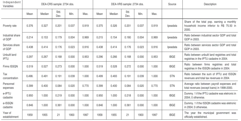
In the second step, to estimate Equation [11], the dependent va-n the second step, to estimate Equation [11], the dependent

va-riable is the natural logaritm of the jackstrapped efficient

sco-res for both DEA variants for the year 2004. Data for matrix X,

containing municipal characteristics come from a cross section

data set for two distinct samples, each one including 2734

muni-cipalities. Both are subsamples of the original sample of 2902 communes. Differences between the original sample and these

subsamples are due to (a) exclusion of outliers by the jackstrap

(12)

E st. E co n., S ã o P au lo , vo

l. 42, n.1, p

. 43-74, j

an.-m ar . 2012 54 M ar ia d a C . S . d e S ou sa , P ed ro L u ca s d a C . A ra ú jo e M ar ia T an n u ri-P ia n to

Table 4.2: Variables

I n d e p e n d e n t

Variables DEA-CRS sample: 2734 obs. DEA-VRS sample: 2734 obs. Source Description

Mean Median Std.

Dev. Min. Max. Mean Median

Std.

Dev. Min. Max.

Grants 0.594 0.599 0.131 0.130 0.993 0.593 0.598 0.131 0.130 0.993 STNa Ratio between non-earmarked grants and total

revenues (except loans) in 2004.

North 0.038 0.000 0.190 0.000 1.000 0.038 0.000 0.190 0.000 1.000 IBGEb Dummy. 1 if located in Northern region; 0

otherwise.

Northeast 0.202 0.000 0.401 0.000 1.000 0.202 0.000 0.401 0.000 1000 IBGE Dummy. 1 if located in Northest region; 0 otherwise.

Center-West 0.090 0.000 0.287 0.000 1.000 0.089 0.000 0.285 0.000 1000 IBGE Dummy. 1 if located in Center-West region; 0 otherwise.

South 0.297 0.000 0.457 0.000 1.000 0.297 0.000 0.457 0.000 1000 IBGE Dummy. 1 if located in Southern region; 0 otherwise.

Metropolitan 0.092 0.000 0.289 0.000 1.000 0.095 0.000 0.294 0.000 1.000 UNDPc Dummy. 1 if located in a metropolitan aera in

2003; 0 otherwise.

Population 0.034 0.013 0.088 0.001 2.333 0.035 0.013 0.094 0.001 2.333 IBGE Estimated population in millions of habitants in 2004.

U r b a n i z a t i o n

rate 0.645 0.680 0.227 0.000 1.000 0.647 0.682 0.227 0.000 1.000 Ipeadata

d Ratio between urban and total population in

2000.

Percapita

income 2.437 2.399 1.075 0.422 11.456 2.450 2.406 1.098 0.422 11.456 Ipeadata

Anual per capita income in thousands of Reais (R$) in 2000.

Poverty rate 0.376 0.327 0.201 0.037 0.919 0.375 0.326 0.201 0.037 0.919 Ipeadata

Share of the total pop. earning a monthly household income inferior to R$ 75.50 in 2000.

Industrial share

of GDP 0.214 0.153 0.179 0.004 0.969 0.215 0.154 0.180 0.004 0.969 Ipeadata

(13)

R es id u a l a n d T ec h n ic a l T a x E i cie n cy S co re s f or B ra zi lia n M u n ic ip a lit ie s 55 E st. E co n., S ã o P au lo , vo

l. 42, n.1, p

. 43-74, j

an.-m

ar

. 2012

Poverty rate 0.376 0.327 0.201 0.037 0.919 0.375 0.326 0.201 0.037 0.919 Ipeadata

Share of the total pop. earning a monthly household income inferior to R$ 75.50 in 2000.

Industrial share

of GDP 0.214 0.153 0.179 0.004 0.969 0.215 0.154 0.180 0.004 0.969 Ipeadata

Ratio between industrial sector GDP and total GDP in 2003.

Services share

of GDP 0.438 0.414 0.176 0.023 0.916 0.438 0.414 0.176 0.023 0.916 Ipeadata

Ratio between services sector GDP and total GDP in 2003.

Unbuilt land

IPTU 0.297 0.267 0.168 0.000 0.953 0.296 0.266 0.168 0.000 0.953 IBGE

Ratio between unbuilt land registries and total registries in the IPTU cadastre in 2004.

Firms ISSQN 0.519 0.527 0.273 0.000 1.000 0.519 0.528 0.272 0.000 1.000 IBGE Ratio between irms registries and total registries in the ISSQN cadastre in 2004.

Tax

concentration 0,498. 0.491 0.191 0.039 1.000 0.499 0.493 0.191 0.039 1.000 STN

Ratio between the sum of IPTU and ISSQN revenues and total tax revenues in 2004.

Personnel

expenses 0.399 0.400 0.084 0.020 0.770 0.399 0.400 0.084 0.020 0.770 STN

Average ratio between payroll expenses and total revenues (except loans) in 1998-2000.

e-IPTU

cadastre 0.950 1.000 0.219 0.000 1.000 0.950 1.000 0.218 0.000 1.000 IBGE

Dummy. 1 if the IPTU cadastre was eletronic in 2004; 0 otherwise.

e-ISSQN

cadastre 0.846 1.000 0.361 0.000 1.000 0.846 1.000 0.361 0.000 1.000 IBGE

Dummy. 1 if the ISSQN cadastre was eletronic in 2004; 0 otherwise.

Year of

establishment 1959 1955 21 1900 1997 1958 1955 21 1900 1997 IBGE

The year the municipal government was oficially established.

(a) National Treasury Secretariat (Secretaria do Tesouro Nacional), “Finanças do Brasil - Dados Contábeis dos Municípios – 2004”; (b) Brazilian Institute of Geography and Statistics (Instituto Brasileiro de Geografia e Estatística), “Perfil dos municípios brasileiros: gestão pública 2004”; (c) United Nations Development Programme, "Atlas do Desenvolvimento Humando no Brasil - 2003"; (d) Database mantained by the Institute for Applied Economic Research (Instituto de Pesquisa Econômica Aplicada, Ipea).

I n d e p e n d e n t

Variables DEA-CRS sample: 2734 obs. DEA-VRS sample: 2734 obs. Source Description

Mean Median Std.

Dev. Min. Max. Mean Median

Std.

Dev. Min. Max.

(14)

5. “Jackstrapped” Results

In this section we present the results from applying the “Jackstrap” procedure described in Section 3 to the data discussed in Section 4. We will first comment the leverage results, then we present the outlier detection process by using the Heaviside step function, and finally we discuss robust DEA efficiency calculations.

5.1. Leverages

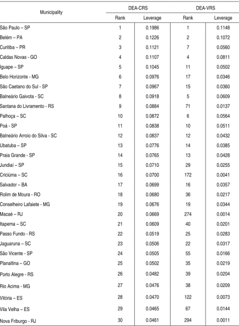
Leverages were calculated for 2902 municipalities for output-orien-ted DEA-CRS and DEA-VRS. Table 5.1 presents leverages for the 30 most influential municipalities. Let us now briefly comment the results. Distinct and non excludable groups of influential DMUs are identified: firstly, we have municipalities for which all output-input ratios were well above the average. Examples of such cases are São Paulo, Belém, Curitiba and Belo Horizonte. In the second group, high leverages are due to a distortion in the ratio between the number of registries in the cadastre of IPTU and the number of municipal em-ployees; this is the case of Balneário Gaivota, Iguape and Balneário Arroio do Silva. Finally, many of those super efficient cities are small towns located in touristy areas close to large and densely populated urban areas. Their valuable real state property as well as a more di-versified offer of services contributes to increase their tax base; they also tend to have lower administrative expenses and hence higher ratio between tax revenues and these expenses. For instance, those rations are 3.9, 4.4 and 5.1, respectively, for Caldas Novas, Ubatuba and Praia Grande whereas the average ratio is only 0.5.

(15)

Municipality DEA-CRS DEA-VRS

Rank Leverage Rank Leverage

São Paulo – SP 1 0.1986 1 0.1148

Belém – PA 2 0.1226 2 0.1072

Curitiba – PR 3 0.1121 7 0.0560

Caldas Novas - GO 4 0.1107 4 0.0811

Iguape – SP 5 0.1045 11 0.0502

Belo Horizonte - MG 6 0.0976 17 0.0346

São Caetano do Sul - SP 7 0.0967 15 0.0360

Balneário Gaivota - SC 8 0.0918 5 0.0609

Santana do Livramento - RS 9 0.0884 71 0.0137

Palhoça – SC 10 0.0872 6 0.0564

Poá - SP 11 0.0838 10 0.0511

Balneário Arroio do Silva - SC 12 0.0837 12 0.0432

Ubatuba – SP 13 0.0776 14 0.0385

Praia Grande - SP 14 0.0765 13 0.0428

Jundiaí – SP 15 0.0710 29 0.0255

Criciúma – SC 16 0.0700 172 0.0041

Salvador – BA 17 0.0699 16 0.0357

Rolim de Moura - RO 18 0.0680 36 0.0217

Conselheiro Lafaiete - MG 19 0.0676 19 0.0344

Macaé – RJ 20 0.0669 274 0.0014

Itapema – SC 21 0.0609 40 0.0201

Passo Fundo - RS 22 0.0519 25 0.0283

Jaguaruna – SC 23 0.0506 22 0.0317

São Vicente - SP 24 0.0505 55 0.0166

Planaltina – GO 25 0.0502 35 0.0219

Porto Alegre - RS 26 0.0482 39 0.0204

Rio Acima - MG 27 0.0476 38 0.0209

Vitória – ES 28 0.0470 122 0.0073

Vila Velha – ES 29 0.0465 67 0.0144

Nova Friburgo - RJ 30 0.0461 294 0.0011

(16)

5.2. Outlier Detection

As mentioned in Section 3, in order to determine which municipali-ties should be considered outliers, we will use a Heaviside rule to re-move outliers (Equation [10]). We rere-moved 66 and 52 municipalities, respectively, for DEA-CRS and the DEA-VRS variants. It should be noted that even when a city displays only local influence such e.g. Planaltina, and hence has little effect on the overall efficiency scores, our “Jackstrap” procedure identifies this anomalous case. As it

per-forms a comparison in B different random “bubbles”, where it turns

out that this city often demonstrates a high level of influence, it obtains a high leverage value. Hence, the “Jackstrap” procedure com-bined with the threshold value defined by the Heaviside function provide a reasonable and automated approximation of the number of outliers. Of course as any cutoff level, this is somewhat arbitrary

but it proved to be, in our experience, a quite robust rule.3

5.3. Eficiency Indexes

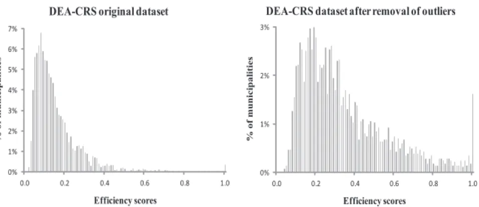
The histograms of efficiency indices obtained through DEA-CRS calculations on the whole dataset and after removing 66 municipa-lities with highest leverage, are shown in Figure 5.1. It is seen that removing the high leverage DMUs generates substantial changes on the overall efficiency scores, whose distribution was originally highly asymmetric and shifted towards the lower efficiency side, as may be expected in the presence of outliers. It should be noted that the number of removed DMUs represents less than 2.5% of the original sample.

3

(17)

Est. Econ., São Paulo, vol. 42, n.1, p. 43-74, jan.-mar. 2012 0%

1% 2% 3% 4% 5% 6% 7%

0.0 0.2 0.4 0.6 0.8 1.0

% of municipalitie

s

Efficiency scores DEA-CRS original dataset

0% 1% 2% 3%

0.0 0.2 0.4 0.6 0.8 1.0

% of municipalitie

s

Efficiency scores DEA-CRS dataset after removal of outliers

Figure 5.1 - Histograms of DEA-CRS Tax Efficiency Scores obtained by using the Original Dataset and after Removing 66 Municipalities with the Highest Leverages

Table 5.2 summarizes the results obtained according to two DEA variants. As expected, the DEA naïve frontiers are formed by a few municipalities. The uncorrected scores are quite distorted, with the majority of efficiencies being close to zero. Here, the presence of outliers not only affects the number of efficient municipalities, but also substantially influences the magnitude of the computed scores, particularly when the DEA-CRS technique is used. Indeed, between the uncorrected score and its equivalent using the Heaviside step function, the average efficiency scores doubles. Observe also that the skewness as well as the kurtosis drops substantially when the ou-tliers are removed, indicating that the distribution of the efficiency scores thus obtained is closest to the normal distribution.

Table 5.2 - Descriptive Statistics for DEA-CRS and DEA-VRS Efficiency Scores

Methodologies Included

observations Eficient (#)

Descriptive Statistics

Mean Median Std. Dev. Skewness Kurtosis

DEA-CRS

Uncorrected 2902 (0)a

10 0.151 0.117 0.124 2.818 12.302

Heaviside 2836 (66) 30 0.344 0.281 0.223 1.133 0.689

DEA-VRS

Uncorrected 2902 (0) 21 0.188 0.148 0.149 2.433 8.314

Heaviside 2850 (52) 113 0.397 0.338 0.240 0.956 0.187

(18)

6. Residual Eficiency Scores

To complement the nonparametric analysis carried out on Section 5, we will investigate the environmental factors affecting the efficiency scores by using OLS and quantile regression methods. The residuals of this regression measure pure technical efficiency after accounting for noncontrollable factors.

6.1. The Econometric Model

Since the efficiency scores are restricted to assume values within

the standard unit interval (0 <λ < 1), the Ordinary Least Squared

(OLS) estimator of the vector of regression parameters will be in-consistent in the sense that it will not converge on probability to the true unknown parameter. However, it has been shown in the

litera-ture that the use of _ln_ as dependent variable leads to unbiased

OLS estimates if the computed scores only assume strictly positive values. Furthermore, when the dependent variable is censored, the OLS estimator of the linear regression parameters will not be consis-tent and such inconsistency worsens with the proportion of censored

observations in the sample.4_{This result implies that the problem}

of inconsistency will not be serious when the number of censored observation is small.

Censored observations may be appropriately tackled using the Tobit model. In this model, parameters are usually estimated by Maximum Likelihood (ML) under the assumptions of normality and homoskedasticity. It is noteworthy that the absence of normality as well as the presence of heteroskedasticity will lead to inconsistent parameter estimates.

In what follows, we shall use the linear regression model instead of the Tobit model. The reasons for that choice are as follows:

Contrary to the Tobit model, estimation in the linear model does

1.

not require the assumption of normality; this assumption can be quite restrictive since we have no prior information about the distribution of the data. Even if is possible to define the Tobit model

using nonnormal distributions, the main shortcoming

remains:

distributional misspecification will render unreliable inference.

4

(19)

The OLS estimator in the linear regression model is unbiased,

2.

consistent and asymptotically normal even under neglected heteroskedasticity of unknown form; the same does not hold for the ML estimator in the Tobit model.

It is possible to obtain an estimate for the covariance matrix of the

3.

OLS estimator of βthat is consistent under both homoskedasticity

and heteroskedasticity of unknown form (see below); hence, one can perform hypothesis tests that are asymptotically valid regardless of the structure of the error variances and of the error distribution. These convenient properties do not hold in the Tobit framework.

The proportion of censored observations in the sample is small

4.

(around 1.8%).

Therefore, we will investigate the exogenous factors, using OLS and quantile regression methods, as introduced by Koenker and Bassett (1978). Just as classical linear regression allows one to estimate mo-dels for conditional mean functions; quantile regression methods offer a mechanism for estimating models for the conditional median

function, and also for other conditional quantile functions. This al-This

al-lows us to investigate the impacts of the conditioning variables on the efficiency scores across different efficiency percentiles. The ba- efficiency scores across different efficiency percentiles. The

ba-sic idea is to estimate the τ-th quantile of efficiency conditional on

the different explanatory variables, assuming that this quantile may be expressed as a linear predictor based on these variables. We con-sidered the following conditional quantiles: 0.10 (percentile 10%), 0.25 (lower quartile), 0.50 (median), 0.75 (upper quartile) e 0.90 (percentile 90%). The dependent variables are the natural logarithms of the efficiency scores for two distinct samples of 2734 Brazilian municipalities computed by using the DEA-CRS and DEA-VRS. Note that the estimated coefficients are conditional to the values obtained by the DEA scores and thus they do not take into account the uncertainty associated to those scores.

(20)

shared by national and regional taxpayers, grants may function then as a substitute for fiscal effort, stimulating inefficiency. To test this hypothesis, we regress tax efficiency scores on grants received by the

communes from higher government spheres (Grants). Our results

strongly confirm those views. The negative and significant coeffi-cients associated to the variable “grants” show that the greater the proportion of municipalities’ expenditure financed by central and state grants, the lower is their tax efficiency. These results

corrobo-rate previous studies5 and reaffirm the inverse relationship between

grants and tax effort and tax efficiency. Concerning the regional

impact, belonging to the Northeast and Northern regions reduces

the municipality’s tax efficiency in the OLS model. This is hardly surprising as these regions concentrate the poorest communes, which are basically financed by grants from higher government spheres. However, quantile estimates moderate this conclusion. Indeed, this result is significant only for the municipalities situated in the

me-dian quantile. Besides, except for the Center-West, the estimated

coefficients are not significant for the last quantiles (τ = 0.75 e τ =

0.90) signaling that for tax jurisdictions relatively efficient, location is not relevant to explain tax variations. Finally, probably due to tax spillovers, belonging to a metropolitan area increases efficiency.

5

Reis and Blanco (1996); Ribeiro (1998); Blanco (1998).

Table 6.1 - Tax Efficiency determinants for Brazilian Municipalities OLS and Quantile Regression Estimates

Independent

Variables Dependent variable: natural log of DEA-CRS scores Dependent variable: natural log of DEA-VRS scores

OLS τ = 0.1 τ = 0.25 τ = 0.5 τ = 0.75 τ = 0.9 OLS τ = 0.1 τ = 0.25 τ = 0.5 τ = 0.75 τ = 0.9 coeff.

p-value coeff. p-value

coeff. p-value

Constant 7.305 10.163 8.196 8.845 7.460 3.015 3.124 7.418 4.183 4.821 1.480 -3.324

0.0000 0.0000 0.0000 0.0000 0.0000 0.0270 0.0034 0.0000 0.0008 0.0001 0.2033 0.0227

Grants -1.322 -1.436 -1.344 -1.228 -1.369 -1.228 -0.562 -0.912 -0.706 -0.651 -0.436 -0.296

< 2e-16 0.0000 0.0000 0.0000 0.0000 0.0000 0.0000 0.0000 0.0000 0.0000 0.0000 0.0172

North -0.080 -0.135 -0.128 -0.070 0.005 0.117 -0.125 -0.327 -0.164 -0.208 0.012 0.061

0.0894 0.0804 0.0515 0.2729 0.9669 0.2693 0.0221 0.0213 0.0008 0.0372 0.9046 0.3637

Northeast -0.089 -0.085 -0.079 -0.108 -0.056 -0.005 -0.084 -0.068 -0.045 -0.111 -0.065 0.061

0.0064 0.0707 0.0818 0.0050 0.2306 0.9198 0.0260 0.2217 0.3209 0.0156 0.1754 0.4179

Center-West 0.155 0.151 0.109 0.135 0.179 0.234 0.052 0.025 0.030 0.049 0.061 0.108

0.0000 0.0060 0.0043 0.0002 0.0000 0.0004 0.1615 0.5868 0.5058 0.2403 0.0718 0.0044

South 0.031 0.142 0.071 0.063 0.024 -0.012 0.032 0.057 0.088 0.043 -0.005 -0.040

(21)

Est. Econ., São Paulo, vol. 42, n.1, p. 43-74, jan.-mar. 2012 Independent

Variables Dependent variable: natural log of DEA-CRS scores Dependent variable: natural log of DEA-VRS scores

OLS τ = 0.1 τ = 0.25 τ = 0.5 τ = 0.75 τ = 0.9 OLS τ = 0.1 τ = 0.25 τ = 0.5 τ = 0.75 τ = 0.9 coeff. p-value coeff. p-value coeff. p-value coeff. p-value coeff. p-value coeff. p-value coeff. p-value coeff. p-value coeff. p-value coeff. p-value coeff. p-value coeff. p-value

Metropolitan 0.112 0.117 0.102 0.107 0.105 0.051 0.099 0.093 0.076 0.083 0.096 0.034

0.0003 0.0089 0.0086 0.0003 0.0184 0.2730 0.0048 0.0067 0.0428 0.0119 0.0013 0.4364

Population 0.269 0.265 0.218 0.378 0.223 0.164 0.713 0.737 0.689 0.919 0.678 0.470

0.0087 0.0060 0.1083 0.0000 0.0813 0.2912 0.0000 0.0000 0.0004 0.0000 0.0000 0.0042

Urbanization rate 0.579 0.726 0.689 0.582 0.491 0.528 0.413 0.690 0.655 0.377 0.252 0.033

< 2e-16 0.0000 0.0000 0.0000 0.0000 0.0000 0.0000 0.0000 0.0000 0.0000 0.0001 0.7293

Per capita income 0.118 0.163 0.145 0.113 0.084 0.039 0.044 0.082 0.064 0.021 0.004 -0.014

0.0000 0.0000 0.0000 0.0000 0.0002 0.0364 0.0258 0.0002 0.0015 0.1369 0.8080 0.4844

Poverty rate -0.464 -0.386 -0.503 -0.542 -0.531 -0.725 -0.820 -0.796 -0.872 -0.963 -1.040 -1.052

0.0000 0.0170 0.0001 0.0000 0.0002 0.0000 0.0000 0.0000 0.0000 0.0000 0.0000 0.0000

Industrial share

of GDP 0.283 0.301 0.199 0.215 0.258 0.383 0.076 0.028 0.062 0.004 0.113 0.205

0.0000 0.0000 0.0080 0.0007 0.0005 0.0001 0.2638 0.7892 0.4014 0.9530 0.0882 0.0595

Services share

of GDP 0.002 0.121 0.067 0.066 0.101 0.115 0.207 0.076 0.217 0.173 0.419 0.505

0.9811 0.2121 0.3941 0.3726 0.2190 0.2490 0.0059 0.4623 0.0141 0.0397 0.0000 0.0000

Unbuilt land IPTU 0.761 0.741 0.669 0.820 0.911 0.777 0.875 0.876 0.808 0.957 0.959 0.753

< 2e-16 0.0000 0.0000 0.0000 0.0000 0.0000 < 2e-16 0.0000 0.0000 0.0000 0.0000 0.0000

Firms ISSQN 0.061 0.058 0.077 0.065 0.041 0.026 -0.015 0.017 0.040 0.026 -0.009 -0.106

0.0382 0.1950 0.0478 0.0596 0.3011 0.5959 0.6675 0.7279 0.3343 0.5182 0.8169 0.0521

Tax concentration -0.032 -0.206 -0.050 -0.007 0.033 0.097 0.036 -0.029 -0.044 0.102 0.049 0.171

0.5289 0.0069 0.4451 0.9027 0.6136 0.2192 0.5425 0.7382 0.5232 0.1405 0.4670 0.0540

Personnel

expenses -0.410 -0.562 -0.522 -0.421 -0.329 -0.256 -0.710 -0.685 -0.662 -0.565 -0.622 -0.501

0.0000 0.0000 0.0000 0.0002 0.0123 0.1013 0.0000 0.0000 0.0000 0.0000 0.0000 0.0009

e-IPTU cadastre 0.143 0.217 0.201 0.131 0.076 0.136 0.078 0.173 0.175 0.015 0.005 0.062

0.0003 0.0000 0.0057 0.0229 0.2355 0.0086 0.0889 0.0003 0.0028 0.7825 0.9038 0.5351

e-ISSQN cadastre 0.105 0.050 0.114 0.108 0.144 0.103 0.078 0.045 0.083 0.095 0.098 0.100

0.0000 0.1662 0.0001 0.0000 0.0000 0.0114 0.0062 0.4003 0.0157 0.0077 0.0180 0.1460

Year of

establishment -0.004 -0.006 -0.005 -0.005 -0.004 -0.002 -0.002 -0.005 -0.003 -0.003 -0.001 0.001

< 2e-16 0.0000 0.0000 0.0000 0.0000 0.0041 0.0001 0.0000 0.0000 0.0000 0.0539 0.0467

Included observations: 2734 Adjusted R2: 0.6059 Residual Std. Error: 0.409 F-statistic: 222.3 p-value: <2.2e-16

Included observations: 2734 Adjusted R2: 0.4234 Residual Std. Error: 0.478 F-statistic: 104.9 p-value: <2.2e-16

Scale variables - Urbanization rate and Population – have a positive

and significant effect upon efficiency. Concerning population, the positive effect is well pronounced for both DEA variants. Hence,

corroborating previous studies [Thirtle et al., 2000; Forsund et al.,

(22)

2005], we found that the size of the tax jurisdiction is one of the most important determinant of tax collection efficiency. As for ur-banization, the positive and significant coefficients attached to this variable probably reflect the concentration of dwellings and econo-mic activity on urban areas as well as the economies of scale on fiscal administration brought about by the economies of agglomeration that characterizes high density areas.

Among tax capacity factors – Industrial share of GDP and Service

share of GDP, Per capita income and Poverty rate – per capita income and poverty rate are the most relevant. The former positively in-fluences efficiency, but its effect decreases across quantiles. Poverty rates – measured by the share of the total population earning a mon-thly household income inferior to R$ 75.50 – are supposed to cap-ture tax base reductions caused by irregular property, tax reduction and exemptions and informality. Negative and significant coefficients support this view for both DEA variants. The Industrial share of GDP is significant only when we use the DEA-CRS variant. As the service tax is an important source of tax collection for

municipali-ties, we would expect the related variable (Service share of GDP)

to influence positively the efficiency scores. Yet, while having the correct sign, the coefficients associated to this variable are signifi-cant only for the DEA-VRS model; and even here, the coefficient for the lowest quantile is not significant. This result may be explained by the fact that, in Brazil, the service sector shows a high degree of informality that leads to fiscal evasion.

Together, scale and capacity factors tend to imply that the price paid by the smallest and poorest tax jurisdictions is reduced efficiency of tax collection. For these units taxation efficiency can be improved mainly by increasing the size of tax jurisdictions and by enlarging their tax base.

Concerning the characteristics of taxpayer payer cadastres for IPTU and ISSQN, two points should be considered. Firstly, as the IPTU rates are higher for unbuilt land, we expect that municipalities with a higher proportion of those lands collect more IPTU revenues, le-ading to higher efficiency scores for these communes. The

estima-ted coefficients for the variable Unbuilt Land IPTU, positive and

(23)

individual taxpayers. To test this hypothesis, we regressed the effi-ciency scores on the proportion of firms in the total registries in the

cadastre of the ISSQN (Firms ISSQN). Our findings weakly confirm

this assumption and only for the lower quantiles of the DEA-CRS variant.

Advocates of tax diversification by local governments have been found in the specialized literature. They argue that such a diversi-fication not only would reduce the reliance on property taxes to fi-nance local expenditures, but should also reduce the deadweight loss of the tax system, for a given revenue, by broadening the tax base and cutting rates. This, together with fiscal illusion that leads to the underestimation of the tax price, should diminish taxpayer resistan-ce to tax increases that would lead to higher tax collection (Becker and Mulligan, 1998; Buchanan and Wagner, 1977). To consider this hypothesis we used the share of property and services taxes on total

tax revenues (Tax Concentration). We expect that the greater this

ratio, the lower the efficiency. The estimated coefficients, although negative, are not significant. Hence we do not find any evidence that diversifying tax base boosts revenue and tax efficiency.

Finally, the rigidity of personnel expenses, measured by the percen-tage of total revenues destined to pay salaries and wages taxes over the period 1998/2000, has a negative impact on tax efficiency. This result is quite robust across quantiles and methodologies. It points out that having a substantial share of revenues earmarked with per-sonnel expenses jeopardize the flexibility required to promote ad-ministrative reforms that include cutting costs and reallocating re-sources into more productivity activities in terms of tax collecting. This rigidity effect is more harmful to inefficient communes located in the lowest quantile.

Let us now investigate the managerial capability of tax jurisdictions. Firstly, we include two dummy variables to capture the moderni-zation of tax administration: the existence of electronic cadastres

of taxpayers for the tax on real state property (e-IPTU cadastre)

and for the tax on services (e-ISSQN cadastre) taxpayers. Here the

CRS and VRS model diverge. When we use the DEA-CRS variant,

coefficients for the dummy e-IPTU cadastre are significant except

for the municipalities on quantile τ = 0.75; thus, having IPTU

(24)

However, with the DEA-VRS model, the coefficients are significant only for the lowest quantiles signaling that once the communes reach a certain level of efficiency in collecting taxes, having electronic ca-dastre is no longer relevant to explain efficiency. As for the dummy

e-ISSQN cadastre, coefficients are positive and significant; never-theless, for the VRS model, this variable is not significant for the extreme quantiles.

Secondly, the recent proliferation of small municipalities in Brazil, which lack not only a sound tax base, but also experience and mana-gerial capability to collect taxes, may lead to reduced tax efficiency. We expect that established municipalities have a better knowledge of its tax base and a more structured tax collecting system. To test for that, we used the year when the municipal government was

offi-cially established (Year of establishment) as a proxy for expertise on

administrative matters, including tax administration. The negative and significant coefficients for all quantiles obtained by both DEA methods, shows clearly that the newer the commune, the less effi-cient in terms of collecting tax revenues, even when we control for other factors such as size and capacity tax factors.

6.2. “Pure” Eficiency Scores

(25)

substan-Residual and Technical Tax Eiciency Scores for Brazilian Municipalities 67

tial amount of ISSQN, related to hotel industry and other tourism activities. These quite particular circumstances do not recommend such municipalities as role models for tax effort, as the non-adjusted efficiency indexes would suggest. Their particular situation cannot be replicated for the typical tax jurisdiction and thus they do not really represent a feasible best practice.

Table 6.2 - DEA-CRS Tax Efficiency Scores for Selected Municipalities - 2004.

Municipality Populationa (#)

Tax revenueb

(103_R$)

Technical

eficiency

score (λk)

Rank

Residual

eficiency

score (Efk)

Rank

Most eficient

Bauru - SP 344,258 52,983 1.0000 1 0.2105 1416

Piracicaba - SP 355,039 78,998 1.0000 1 0.2330 1134

Guarapari - ES 102,089 14,247 1.0000 1 0.2357 1103

Águas de Lindóia - SP 18,289 6,914 1.0000 1 0.2645 791

Franca - SP 315,770 40,710 1.0000 1 0.2678 763

Arroio do Sal - RS 6,423 2,467 1.0000 1 0.2830 655

Arujá - SP 70,248 14,742 1.0000 1 0.3051 500

Águas de Santa Bárbara - SP 5,907 2,740 1.0000 1 0.3119 459

Itu - SP 149,758 26,496 1.0000 1 0.3162 438

Rio Grande - RS 193,789 30,365 1.0000 1 0.3213 410

Least eficient

Ponto dos Volantes - MG 11,349 157 0.1556 2259 0.2227 459

Ibirapuã - BA 6,483 374 0.1788 2073 0.2603 253

Caatiba - BA 18,484 390 0.1911 1972 0.2984 140

Cacimbinhas - AL 8,600 206 0.1853 2017 0.2820 182

Plácido de Castro - AC 15,931 77 0.1449 2338 0.2245 448

Piranhas - AL 22,854 465 0.1774 2085 0.2786 193

Carnaubeira da Penha - PE 10,007 244 0.0919 2684 0.1991 683

Granjeiro - CE 5,578 138 0.1639 2177 0.3123 116

Olho D’Água do Piauí - PI 2,113 49 0.1372 2386 0.2457 324

Tarrafas - CE 8,751 205 0.1437 2345 0.2746 204

Sources: (a) Brazilian Institute of Geography and Statistics (Instituto Brasileiro de Geografia e

Estatística, IBGE), “Perfil dos municípios brasileiros: gestão pública 2004”; (b)

Natio-nal Treasury Secretariat (Secretaria do Tesouro Nacional, STN), “Finanças do Brasil

(26)

For the most inefficient tax jurisdictions, “pure” efficiency indexes are superior to the non-adjusted ones. Indeed, the worse the commu-ne-specific conditions the greater the rise in the residual efficiency score. The typical municipality situated at the bottom of the effi-ciency distribution is small, poor, with a very limited tax base. Their adverse environment makes them look much more inefficient than they really are. In that sense, residual scores present a more com-plete picture of the municipality’s tax effort because the magnitude of the non-adjusted indexes reflects factors other than managerial efficiency. Hence, when we take into account environmental factors, there is a convergence between the scores across communes.

Table 6.3 shows the descriptive statistics for residual efficiency sco-res as well as the rank correlations between those scosco-res and the ones computed by the jackstrapped method. Firstly, to track the mobility of tax jurisdictions across different definitions of efficiency, we computed the rank correlations between DEA jackstrapped sco-res and sco-residual efficiency scosco-res. The rank correlations are 0.60 and 0.75, respectively, for the CRS and VRS variants. Secondly, for most communes, “pure” scores are lower than the “gross” ones. For instance, under the DEA-CRS and DEA-VRS variants, only 34% and 2%, respectively, of the municipalities have a “gross” efficiency score inferior to the residual one. The fact that this proportion is much lower – for all population groups – when the DEA-VRS was used is consistent with the fact that this variant envelops the DEA-CRS model.

(27)

Methodologies and Population Groups

Obs. (#)

Rank

Correlation λk

and Efk

Obs. for

which λk

> Efk (%)

Efk Descriptive Statistics

Mean Median Std.

Dev. Skewness Kurtosis

DEA-CRS 2734 0.605 66% 0.235 0.215 0.107 2.198 9.159

0 to 49,999 2343 0.611 64% 0.236 0.215 0.105 2.124 8.790

50,000 to 299,999 352 0.616 82% 0.234 0.207 0.117 2.525 10.599

>300,000 39 0.535 87% 0.235 0.218 0.101 2.624 10.690

DEA-VRS 2734 0.750 98% 0.173 0.152 0.096 2.512 10.776

0 to 49,999 2334 0.748 97% 0.173 0.152 0.096 2.580 11.526

50,000 to 299,999 356 0.793 100% 0.170 0.147 0.096 2.141 6.367

>300,000 44 0.704 100% 0.187 0.159 0.083 1.841 4.208

When we disaggregate our results by size of the tax jurisdiction, we have a quite interesting result. Managerial tax efficiency, here measured by residual (“pure”) efficiency indexes, does not seems to differ significantly across different classes of population. Indeed the mean score variations are low among municipalities of different si-zes. This result is only apparently surprising. It means that efficiency heterogeneity in terms of tax collection observed among Brazilian communes, particularly among small ones, is mainly caused by their specific environmental conditions, rather than by differences in their tax administration.

Our findings suggest that to improve municipal tax efficiency we have to adopt different strategies according to the particular condi-tions faced by the communes. Those with a substantial tax capacity and better socioeconomic conditions might improve efficiency by better management of controllable inputs by adopting programs that boost tax collection and reduce evasion. However, communes lacking both, tax capacity and good economic conditions, face a more dif-ficult challenge, as the tax inefficiencies are due to external factors, outside their control. In such cases, improving tax administration should be part of a more coordinated strategy aiming to improve local development that would permit to expand and/or create their tax base.

(28)

Notice also that the positive kurtosis for all measures of tax effi-ciency indicate that their effieffi-ciency distributions have fat tails re-lative to the normal distribution. This phenomenon is so intense for the small cities that several of them present residual efficiency scores higher than the high scores of the big cities, indicating once again that their adverse environment and socioeconomic conditions accounts for most of their overall inefficiency.

Lastly, to summarize our results, Table 6.4 presents the computed aggregate tax efficiency scores for both one-stage and two-stage ap-proaches, measured as a weighted mean of individual scores. The

weights are given by the tax share of the k-th municipality on total

tax revenue.

Table 6.4 - Aggregate Tax Efficiency Scores for Brazilian Municipalities 2004.

Methodologies

Aggregate Tax Eficiency Scores

Technical Eficiency (λk) Residual Eficiency (Efk)

DEA-CRS 0.684 0.231

DEA-VRS 0.736 0.164

As we see, the overall tax performance of Brazilian municipalities has been quite disappointing. The low efficiency indexes here - the “gross” as well as the residual ones - show clearly that there is a wide space for increasing municipal tax effort. This conclusion is valid for small and larger cities as well as rich and poor ones. This result seems to imply that the Brazilian municipal tax jurisdiction lack appropriate incentives to adopt efficient tax systems by better exploring their tax base (when they have one), rationalizing their tax structure, and by reducing tax avoidance and evasion.

7. Conclusion

(29)

in our DEA calculations, we included those factors in the analysis. To that end, we used econometric methods (including quantile re-gression) to investigate how the excluded variables influenced the computed “gross” efficiency scores. The econometric results proved to be quite robust to the nonparametric efficiency variants used as dependent variable.

Corroborating previous results, gross tax efficiency results show a clear relationship between the municipality’s size and urbanization and its efficiency scores. Scale variables – urbanization rate and population – have a positive and significant effect upon efficiency. Indeed, under both DEA variants, smaller cities tend to be less effi-cient than larger ones hence indicating that size of the tax jurisdic-tion is a relevant determinant of tax efficiency. Tax capacity factors also proved to be a key determinant of tax efficiency. Together, scale and capacity factors tend to imply that the price to pay for smaller tax jurisdictions is reduced productivity of tax collection. Hence, te-chnical productivity of taxation could be improved mainly by small

unitsbecoming larger.

Our findings also suggest the existence of moral hazard problem in relationship between local tax jurisdictions and the central/state governments. Fiscal transfers granted to municipalities seem to act as a substitute for tax effort so that national taxpayers can finance local expenses. This point is particularly relevant for Brazil, whe-re the design of fiscal transfers is totally disconnected from the municipalities’ performance regarding tax collection. Hence, if one wants to boost tax efficiency, it is imperative to change the rules for conceding these grants.

(30)

References

Bahl, R. W. (1971). “A Regression Approach to Tax Effort and Tax Ratio Analysis”. IMF Staff Papers, n. 18, p. 570-607.

Battese, G. (1992). “Frontier production functions and technical efﬁciency: a survey of empirical appli -cations in agricultural economics”. Agricultural Economics, v.7, p. 185-208.

Baretti, C., Huber, B., and Lichtblau, K. (2000). “A tax on tax revenue: the incentive effects of equalizing transfers: Evidence from Germany”. Working Paper 333, CESifo, Munich.

Barros, C. P. (2007). “Technical and allocative efﬁciency of tax ofﬁces: a case study”. Journal of Public Sector Performance Management, 1, pp. 41-60.

Becker, Gary S. and B. C. Mulligan (1998). “Deadweight Costs and the Size of Government”. Cambridge. NBER Working Paper Series. Working Paper 6789. November.

Bird R. M., Tarasov A. V. (2004). "Closing the gap: ﬁscal imbalances and intergovernmental transfers in developed federations". Environment and Planning C: Government and Policy, v. 22(1) 77 – 102. Blanco, F. A. (1998). “Disparidades Interregionais, Capacidade de Obtenção de Recursos Tributários,

Esforço Fiscal e Gasto Público no Federalismo Brasileiro”. XX Prêmio BNDES de Dissertação de Mestrado, Rio de Janeiro: BNDES.

Boadway, R, I. Horiba and R.Jha (1999). “The provision of public services by government funded decentralized agencies”. Public Choice, v. 100, 157–184.

Buchanan, J., and Wagner, R. E. (1977). “Democracy in Deﬁcit: The Political Legacy of Lord Keynes”. New York: Academic Press.

Cazals, C., J.P. Florens and Simar, L. (2002). “Nonparametric Frontier Estimation: A Robust Approach”. Journal of Econometrics, v. 106, 1-25.

Charnes, A., W. W. Cooper and E. Rhodes (1978). “Measuring Efﬁciency of Decision Making Units”. European Journal of Operational Research, 1, 429–44.

Cherchye, L., T. Kuosmanen and G. T. Post (2000). “New Tools for Dealing with Errors in Variables in DEA”. CES Discussion Paper 0006.

Deprins, D., L. Simar and H. Tulkens. (1984). “Measuring Labor Efficiency in Post Offices.” In: M. Färe, R., S. Grosskopf and C. K. Lovell (1985). “The Measurement of Efficiency of Production”. Boston:

Kluwer-Nijhoff Publishing.

Esteller-Moré, A (2005). “Is There a Connection Between the Tax Administration and the Political Power?”. International Tax and Public Finance, pp. 639-663.

Farrell, M. J. (1957). “The Measurement of Productive Efﬁciency”, Journal of the Royal Statistical Society, A CXX, Part 3.

Førsund, F.R., S. Kittelsen and F. Lindseth (2005). “Efﬁciency and Productivity of Norwegian Tax Ofﬁces”. Memorandum 29/2005, University of Oslo, Department of Economics.

Greene, W.H. (1981). “On the asymptotic bias of the ordinary least squares estimator of the Tobit model”. Econometrica, v. 49, 505-513.

Gasparini, C. E., Melo, C. S. L. de (2004). “Equidade e Eficiência Municipal: uma Avaliação do Fundo de Participação dos Municípios – FPM”. VIII Prêmio Tesouro Nacional. Brasília: ESAF. Instituto Brasileiro de Geografia e Estatística – IBGE (2005). “Perfil dos municípios brasileiros: gestão

pública 2004”. Rio de Janeiro: IBGE.

Jha, R., M. S. Mohanty S. Chatterjee and P. Chitkara (1999). “Tax effciency in selected Indian states”. Empirical Economics, 24:641-654.