Regional Labor Market Differences in
Brazil and Search Frictions: Some
Structural Estimates
*
Paulo Felipe de Oliveira,
†
José Raimundo Carvalho
‡
Contents: 1. Introduction; 2. Regional Differences in Brazilian Labor Markets; 3. Empirical
Implementation of Job Search Models; 4. Empirical Analysis; 5. Results; 6. Concluding Remarks. Keywords: Search Theory, Regional Differences, Structural Econometrics.
JEL Code: J64, C14, C41.
We estimate an equilibrium job search model for six metropolitan areas located in different regions of Brazil. Two mechanisms of wage determination are con-sidered: wage posting by monopsony firms and Nash bilateral bargaining. In order to estimate the model, we use the non-parametric method developed by Bontemps, Robin, & van den Berg[2000. Equilibrium search with continuous productivity dispersion: Theory and nonparametric estimation. International Economic Review, 41(2), 305–358]. There is significant heterogeneity among the estimated structural parameters for these regions. We succeed in rationaliz-ing some well-known regional differences in wages, unemployment rates and productivity prevalent in Brazilian labor markets, thus offering new interpreta-tions. Metropolitan regions in the Northeast have much lowerλ0(arrival rate
of wage offers for unemployed workers) andλ1 (arrival rate of wage offers for
employed workers)vis a visareas in the South or Southeast regions. This is a new, and much more precise, result worth considering on the regional inequal-ity debate in Brazil. Regional inequalinequal-ity in wages, besides being an outcome of its regional human capital distribution, can be rationalized as inequality of search frictions brought by differences inλ1. We found a key (indirect) role for
search frictions when analysing productivity differences as well. Since search frictions impact simultaneously on monopsony power as well as on productiv-ity, in order to understand better regional productivity differences we must deepen our analysis on how these structural parameters are differentiated by regions. Labor market frictions add important insights into the regional de-bate, something not captured by more traditional econometric reduced form approaches.
*This paper has been circulating under the title “Estimation of an Equilibrium Search Model with Productivity Dispersion: a
Regional Analysis for Brazil”. We thank participants from the 33rdMeeting of the Brazilian Econometric Society, 2011, and
the 6thCAEN-EPGE Meeting of Public Policy and Economic Growth, 2013, for valuable comments and suggestions. The usual
disclaimer applies.
†Ministério do Desenvolvimento, Indústria e Comércio Exterior. I would like to thank CNPq, Brazil.
Estimamos um modelo de procura de emprego de equilíbrio para seis regiões metro-politanas localizadas em diferentes regiões do Brasil. Dois mecanismos de determi-nação dos salários são considerados: postagem de salários por empresas monopsô-nicas e negociação bilateral a la Nash. Para estimar o modelo, usamos o método não-paramétrico desenvolvido porBontemps, Robin, & van den Berg[2000. Equili-brium search with continuous productivity dispersion: Theory and nonparametric estimation. International Economic Review, 41(2), 305–358]. Existe heterogenei-dade significativa entre os parâmetros estruturais estimados para essas regiões. Con-seguimos racionalizar diferenças regionais já bem conhecidas nos salários, taxas de desemprego e produtividade prevalentes nos mercados de trabalho brasileiros, ofe-recendo assim novas interpretações. Regiões metropolitanas do Nordeste possuem λ0(taxa de oferta de salários para trabalhadores empregados) eλ1 (taxa de oferta
de salários para trabalhadores empregados) muito menoresvis a visaquelas encon-tradas nas regiões Sul ou Sudeste. Este é um resultado novo e muito mais preciso que vale a pena ser considerado no debate regional da desigualdade no Brasil. A de-sigualdade regional nos salários, além de ser resultado da distribuição regional de capital humano, pode ser racionalizada através da desigualdade de fricções trazidas por diferenças entreλ1’s. Evidenciamos também um papel (indireto) importante das
fricções de busca quando se analisam as diferenças de produtividade. Como os atri-tos de busca impactam simultaneamente sobre o poder de monopsônio, bem como sobre a produtividade, a fim de entender melhor as diferenças de produtividade regi-onais, devemos aprofundar nossa análise sobre como esses parâmetros estruturais são diferenciadas por regiões. Fricções no mercado de trabalho adicionam importan-tesinsightsao debate, algo que não é capturado por abordagens econométricas de forma “reduzidas” mais tradicionais.
1. INTRODUCTION
Job search theory considers the labor market an environment of imperfect information. This implies that transactions in this market need time and other resources to be held, since agents are not fully informed about the opportunities and characteristics which are relevant to the transaction (seeEckstein & van den Berg,2007andRogerson, Shimer, & Wright,2005). Hence, these models serve as a substitute for the analysis of labor markets outside the neoclassical paradigm of labor supply, which precludes the possibility of involuntary unemployment.
In an environment of imperfect information, firms can exploit the fact that workers are not fully informed about all opportunities and thus offer wages which are lower than the value of labor produc-tivity, even in a situation where firms and workers are homogeneous (Burdett & Mortensen,1998). Thus, the prevailing wage may be smaller than in an environment of perfect competition, where wages would be equal to the marginal labor productivity. Moreover, from a structural estimation perspective, it is possible to analyze jointly, in a context of market equilibrium, labor market issues such as arrival rates of job offers for employed and unemployed workers, the separation rate of employment relations, firm’s productivity, and monopsony power. Hence, one can make an attempt to infer the factors that would account for differences in unemployment rates between regions or would influence the level of frictions present in the labor market on wages, for example.
accordance with stylized facts about regional inequality of Brazilian markets (seeReis & Barros,1990, Savedoff,1990,Savedoff,1995,Azzoni & Servo,2002,Queiroz & Golgher,2008, andFreguglia & Menezes-Filho,2012). It also present new insights and hints on why such inequalities might exist.
The productivity debate in Brazil is also object of our analysis. In order to do that we confront two possible wage determination mechanisms: wage postingex anteby monopsonist firms that set wages unilaterally, based inBontemps, Robin, & van den Berg(2000), and Nash bilateral bargainingex post, based inMortensen(2003). The methodology used to estimate the model is the nonparametric method ofBontemps et al.(2000), which enables us to estimate the model without assuming any parametric probability distribution of firms’ productivity. Our results show the superiority of the Nash bilateral bargaining model, both in terms of fit as well as in terms of replicating stylised facts about regional productivity differences.
Although empirical analysis based on structural estimation of search models are already quite devel-oped internationally,1in Brazil, the literature is virtually nonexistent, andCarvalho(2012) andOliveira (2011) are rare examples of structural analysis of a search model using Brazilian data (Survey of Living Standards–PPV). However, our paper not only develops and estimates a search model but also suggests that this methodology can shed important insights into the debate over regional labor market differ-ences.
The empirical analysis in this study confirms and shows significant differences between regions. Some regions have a higher expected unemployment duration, as the metropolitan areas of Salvador and Rio de Janeiro, where the expected completed durations of unemployment are equal to approximately eleven months, while for the metropolitan region of Belo Horizonte this term is near four months. In the metropolitan area of Recife, employed workers have a low transition rate to jobs that pay higher wages, while regions such as São Paulo and Porto Alegre have a relatively high mobility. Despite these results, our methodology shows its strength when we are able to rationalize some well-known regional differences in Brazilian labor markets by means of deep structural parameters. Clearly, the role of la-bor market frictions, internal lala-bor market dynamics and market organization (monopsony level) add important insights into the debate.
In terms of productivities, depending on the type assumed in the wage determination, we arrive at different conclusions. The model with wage posting inferred high-productivity levels, a result also found byMortensen(2003) andShimer(2006), and the bilateral bargaining has more plausible and theoretically admissible values that do not violate any theoretical restriction. In the case of bargaining, the metropolitan region of São Paulo has the highest level of productivity and Recife has the lowest level. When compared to Recife, the distribution of firms’ productivity in São Paulo is also more dispersed. We believe that our estimates have the potential to contribute to the long-standing debate about regional differences in Brazilian labor markets (see, among others,Reis & Barros,1990,Savedoff,1990,Savedoff, 1995,Azzoni & Servo,2002,Queiroz & Golgher,2008, andFreguglia & Menezes-Filho,2012).
Besides this introductory section, the paper is organized as follows: Section 2presents a brief de-scription of the recent debate about regional differences in Brazilian labor markets, focusing on three main labor market outcomes: wages, unemployment rate and productivity.Section 3reviews the theo-retical and empirical literature on structural estimation of search models in the labor market.Section 4 addresses the empirical part of the paper and it is split into three subsections: Theoretical Background, Data Set and Structural Estimation.Section 5presents and discusses the main structural estimates and, finally,section 6draws some final considerations.
2. REGIONAL DIFFERENCES IN BRAZILIAN LABOR MARKETS
According toAzzoni & Servo(2002), among others, Brazil has a high level of regional inequality and the prospects of any improvement from the present to the medium run are at best disappointing. Although
this regional inequality can be discussed from many perspectives, income inequality (more specifically labor income) is the subject of most scrutiny in the literature.Azzoni & Servoassert that
The Northeast region of Brazil is home to 28% of the Brazilian population in 2000; it pro-duced only 13% of the Brazilian GDP in 1998. The rich Southeast region represented 43% of the total population and produced 58% of GDP. Per capita income in the Northeast was 54% below the national average while in the Southeast it was 36% above that level. The poorest state, Piaui, in the Northeast region, had a per capita income level 5.6 times lower than the richest state, Sao Paulo, in the Southeast region.
Hence, it is a well-established fact that Brazilian labor markets are very heterogenous.
A less developed argument is that, besides earnings differences, regional inequality in Brazilian la-bor markets can be found, at least indirectly, when one looks at other indexes such as unemployment rates, unemployment duration, productivity differences, among other economic variables. In fact, labor market differences in Brazil is by no means a recent trend. As a matter of fact, much of our regional dispar-ities can be traced back to colonial times, where the North-South (more precisely, Northeast-Southeast) disparities started up, enlarging during the last decades of development (Araújo & Lima,2010). In that sense, we think that a brief literature review on regional differences in Brazilian labor markets that con-siders those aspects of heterogeneity as well as the recent path of regional inequality is important for a better understanding of our arguments.
In order to start understanding regional differences in Brazilian labor markets during the first decade of the 21st century, we need to understand the macroeconomic environment surrounding that period. The Brazilian economy started to recover from a period of stagnation during the 1980s and mid-1990s, initiating a period of modest growth from 1995 on. But it was only during the period from 2004 up to 2008 that we observe a real acceleration in its growth rate. Basically, this acceleration took place simultaneously with
[…] the influence from the growth conditions of the world economy and domestic demand driven by real increases in the minimum wage, the expansion of personal credit and higher volume of federal cash transfers resources, and the multiplier effects of export activity benefited from major expansion of foreign demand for industrial and agricultural commodi-ties. (Araújo & Lima,2010)
The rest of this section discusses three aspects of regional labor market differences in Brazi: wages, unemployment rate and productivity.
2.1. Wage Differences
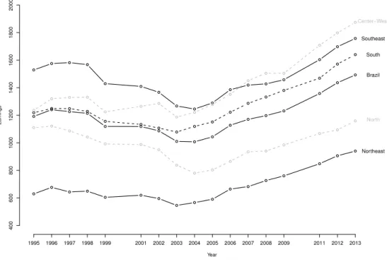
Although the debate about income inequality is well established among Brazilian scholars (see, among others,Barros & Mendonça,1995,Langoni,2005,Barros, Foguel, & Ulyssea,2006), the debate about in-come inequality with an emphasis on regional differences on earnings has received much less attention. Few papers likeReis & Barros(1990),Savedoff(1990),Savedoff(1995),Azzoni & Servo(2002),Queiroz & Golgher(2008), andFreguglia & Menezes-Filho(2012) treat in an explicitly manner the stark earnings differences among Brazilian regions, pointing out the important role that human capital unequal dis-tribution has on this inequality as well as other observed and unobserved individual heterogeneities.2 Table 1shows the evolution of the average monthly earnings between regions in Brazil.
Table 1andFigure 1show clearly that the Southeast region was the leader in labor productivity until 2007 (only surpassed by the Center-West mainly due to agricultural productiviy) and the North-east region remains at the last place. Also, the gap between SouthNorth-east and NorthNorth-east remains almost unchanged.
2However, some evidence point out to the fact that these differences are considerably reduced once we control for unobserved
Table 1.Average Monthly Earnings at main job of occupied population 16 years or older.
Region 2004 2005 2006 2007 2008 2009 2011
Brazil 1,007.68 1,043.71 1,127.58 1,170.46 1,197.75 1,231.56 1,357.84
North 780.41 803.42 865.49 934.61 940.49 985.38 1,067.22
Northeast 566.77 590.78 664.76 682.43 726.74 760.33 848.52
Southeast 1,245.6 1,289.6 1,385.48 1,419.14 1,427.75 1,457.84 1,603.35
South 1,119.33 1,151.6 1,222.12 1,286.72 1,332.61 1,380.37 1,468.88
Center-West 1,220.96 1,277.92 1,352.02 1,451.23 1,504.83 1,504.43 1,707.97
Note:R$ of 09/2013 – INPC. Source:IBGE/PNAD.
Figure 1.Mean Monthly Earnings at main job of occupied population 16 years or older.
Year
Ear
nings
Brazil
400
600
800
1000
1200
1400
1600
1800
2000
1995 1996 1997 1998 1999 2001 2002 2003 2004 2005 2006 2007 2008 2009 2011 2012 2013 North
Northeast Southeast
South Center−West
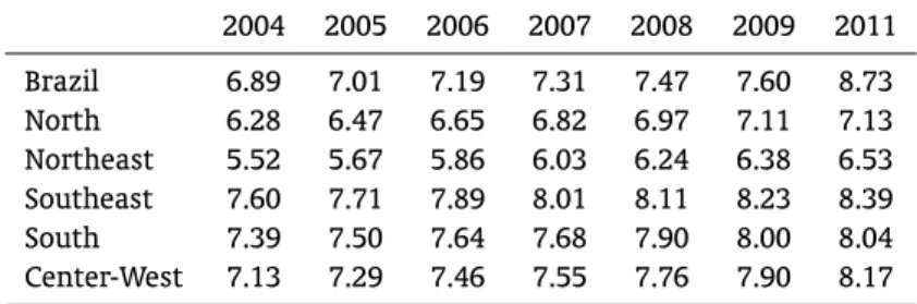
Many Brazilian authors suggest inequality of human capital distribution as the main explanation for that situation (see, among others,Reis & Barros,1990,Barros & Mendonça,1995,Duarte, Ferreira, & Salvato,2004, andBarros et al.,2006).Table 2presents the mean number of years of education by region. Overall, these figures support the human capital explanation for wage income inequality among regions. However, as many others have argued convincingly other explanations like unionization (Arbache,1999), quality of education (Behrman & Birdsall,1983), bargaining and mark-up power (Amadeo,1994), and individual unobserved heterogeneity (Freguglia & Menezes-Filho,2012) are important to understand wages differences.
2.2. Unemployment Rate Differences
Table 2.Mean Years of Education 16 years or older.
2004 2005 2006 2007 2008 2009 2011
Brazil 6.89 7.01 7.19 7.31 7.47 7.60 8.73
North 6.28 6.47 6.65 6.82 6.97 7.11 7.13
Northeast 5.52 5.67 5.86 6.03 6.24 6.38 6.53
Southeast 7.60 7.71 7.89 8.01 8.11 8.23 8.39
South 7.39 7.50 7.64 7.68 7.90 8.00 8.04
Center-West 7.13 7.29 7.46 7.55 7.76 7.90 8.17
Source:PNAD/IBGE.
Corseuil et al.(1997) presents an analysis of local and national unemployment rates. The authors attempt to measure how aggregate shocks in the Brazilian economy impact on regional labor markets. Corseuil et al.(1997) depart from three basic premises: the sensitivity of regional unemployment with respect to shocks at the national employment; decomposition of regional unemployment into aggregate, regional and industry factors; and fluctuations in regional unemployment.
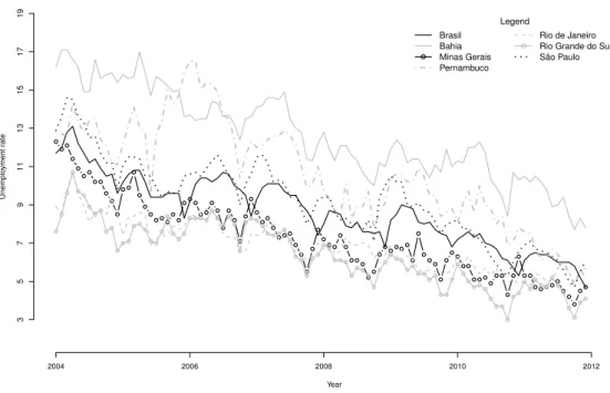
They draw to main conclusions: i) aggregate shocks are more important than structural regional shocks to explain unemployment dynamics; and ii) it is not easy to define in a clear and unambiguous way whose region has greater natural unemployment rate. So, althoughCorseuil et al.(1997) are a benchmark in the national literature about regional differences in unemployment dynamics, it falls short over achieving a clear regional explanation for unemployment dynamics. In light of this fact, we resort to more simple empirical evidence in order to have a glimpse on some sort of regional unemployment differences.Table 3andFigure 2give us some hints.
A first clear trend is the constant decline on unemployment rate over all regions under analysis. A second, and in a sense, dissapointing pattern, is the fact that for Bahia, Pernambuco (both at the Northeast region) and São Paulo (Southeast region), unemployment rates stay higher than the national level all over the years from 2004 up to 2010. So, this signals that any sort of regional disparity in unemployment rate would be a little hard to back up. Notwithstanding that, we could tentatively try to support a view that Southwestern states like Rio de Janeiro and Minas Gerais (with the exception of São Paulo) have lower unemployment rates than those states in the Northeast.
2.3. Productivity Differences
The 1990s brought an unprecedent period of structural change in Brazil’s economy. The process of openness of Brazilian economy prompted many changes in the industrial sector, bringing the neces-sary productive modernization and technological gains in order to be competitive at a global level (see, Feijó & Carvalho,2002,Galeano & Wanderley,2013a,2013b). In terms of labor productivity, at first we saw considerable gains overall. However, these initial gains faded away by the beginning of the 2000s. According toGaleano & Wanderley(2013a), the decrease in labor productivity that started around 1998– 2000 was due mainly to the considerable growth on the number of occupied workers.
The first decade of the 21st century witnesses, from 2002 on, first a fall in labor productivity driven by a decrease on the value of industrial transformation coupled with a increment on the number of occupied workers. From 2002 up to 2005, the growth rate of labor productivity was zero, although we saw a little recovery by the end of the decade. By 2007–2008, labor productivity reached the same value as of 1996. Such evidence of a falling labor productivity prompted some authors to question the very process of openness of Brazilian economy as a beneficial one (see, among others,Galeano & Wanderley, 2013a,2013b,Schettini & Azzoni,2013, andCavalcante & De Negri,2014).
Table 3. Unemployment Rate.
Metropolitan Area 2004 2005 2006 2007 2008 2009 2010 2011
Salvador – Bahia 16.03 15.38 13.57 13.43 11.36 11.37 10.79 9.23
Belo Horizonte – Minas Gerais 10.63 8.98 8.57 7.35 6.43 6.39 5.39 4.68
Recife – Pernambuco 12.68 13.41 13.96 11.78 8.97 9.84 8.46 6.20
Rio de Janeiro – Rio de Janeiro 9.03 7.81 7.83 7.09 6.75 5.96 5.53 5.30
Porto Alegre – Rio Grande do Sul 8.64 7.50 8.12 6.97 5.83 5.42 4.46 4.44
Sao Paulo – Sao Paulo 12.63 10.44 10.60 9.88 8.53 8.91 6.73 6.09
Brazil 11.48 9.83 9.98 9.29 7.89 8.08 6.74 5.98
Source:IpeaData.
Figure 2.Unemployment Rate.
2004 2006 2008 2010 2012
Year
Unemplo
yment r
ate
3
5
7
9
11
13
15
17
19
Legend Brasil
Bahia Minas Gerais Pernambuco
Rio de Janeiro Rio Grande do Sul São Paulo
regional impacts, say, spatial reallocation of industrial activity among regions of Brazil. The main effect was a deconcentration of industrial activity from the South and Southeast regions towards North and, mainly, Northeast regions. Actually, the growth rate of labor productivity from the Southeast region was lower than those of all other regions, contributing to slow down the process of regional inequality.
Notwithstanding that increase in labor productivity of all regionsvis a visthe more developed South-east region, with the exception of the North region (whose industry is driven mainly by a massive pro-gram of fiscal incentives and “Zona Franca de Manaus” in the state of Amazonas) there is an important gap on labor productivity (seeTable 4). Of course, a gap in labor productivity is well known for having deep impacts on growth and development and for posing an obstacle to regional development, since at leastKaldor(1970).
Table 4.Industrial Labor Productivity in 2010.
Extractive Industry
Transformation Industry
Brazil 145.64 26.97
North 448.44 37.21
Northeast 57.78 19.69
Southeast 156.84 30.81
South 18.15 21.87
Center-West 86.38 24.59
Notes:1,000 R$ of 1996.
Source:Galeano & Wanderley(2013b).
as our econometric estimation exercises shed light on the deep relationships brought by the modern search theory. Next section briefly digresses over the empirical implementation of equilibrium search models.
3. EMPIRICAL IMPLEMENTATION OF JOB SEARCH MODELS
We start by summarizing the two main different approaches that lead to wage dispersion in job search models as a response toDiamond(1971)’s degeneracy of the wage offer distribution. The first approach is represented by the model byAlbrecht & Axell(1984). The wage dispersion occurs atAlbrecht & Axell (1984) due to the fact that workers are heterogeneous with respect to the value attributed to leisure (or the opportunity cost of labor). Thus, workers differ in the value of reservation wage. By offering a higher wage, the firm increases the level of employment in steady state, but reduces the profit per worker. It is, then, possible that firms which offer different wages have equal profits, enabling the existence of an equilibrium with wage dispersion. Therefore, in this model, the support of the wage offer distribution is equal to a subset of the reservation wages of workers.
The second approach is based mainly onBurdett & Mortensen(1998). The main result ofBurdett & Mortensenis an equilibrium with wage dispersion even if workers and firms are identical. The disper-sion is produced by the possibility of on-the-job search. Firms can offer wages which are higher than the reservation wage because it would also attract more workers from other employers. That is, the labor supply curve for the firm is upward sloping. Thus, using the isoprofit assumption for firms that offer different wages, it is possible to get an equilibrium where the wage distribution is not degenerate on the common reservation wage, avoiding theDiamond(1971) paradox. Finally, the model byBurdett & Mortensen(1998) is characterized as a model of wage posting. In other words, firms unilaterally decide the wage offer and bargaining between workers and employers will not occur.
The study byvan den Berg & Ridder(1998) followsBurdett & Mortensen(1998) model. The authors consider that the labor market is segmented in relation to some characteristics of workers and, in turn, each segment can be considered a labor market. Thus, it is considered that in each segment workers and firms are homogeneous, but there is heterogeneity between markets. This heterogeneity is important to adjust the model to data. The analysis is performed from a panel data of employed and unemployed workers in the Netherlands. From the estimates of the theoretical model’s parameters, the authors es-timate the degree of monopsony in firms, effects of minimum wages variations and the factors that de-termine the wage dispersion. The degree of monopsony is estimated between 10% and 17%. Employed workers have a high arrival rate of wage offers that influences the competition by firms, reducing their power. Moreover, the results indicate that only 22% of the observed wage dispersion is explained by the friction in the labor market.
Bontemps et al.(2000) extend theBurdett & Mortensen(1998) model by assuming that firms are heterogeneous in terms of labor productivity and introduce a continuous distribution of firms’ produc-tivities. These authors argue that in reality firms use different technologies and that the assumption of identical firms generates a theoretical distribution of wages with an increasing density, which would be as opposed to data which shows that the highest wages occur at a low frequency. Moreover, the au-thors do not allow the workers to be heterogeneous due to the fact that, from the evidence ofEckstein & Wolpin(1990), this type of heterogeneity explains a small fraction of the variation in wages. Then, the wage dispersion is caused by search friction in the labor market and the difference in the firms’ productivity.
The model is estimated by a nonparametric method consisting of three stages and has the advan-tage of the frictional parameters being estimated consistently independent from the strategy that firms adopt. The model is estimated for some sectors of the French economy (transportation, food, equipment, etc.) using microdata from workers and confronting the results with data from employers. The results indicate that firms exploit friction in the labor market, implying a high monopsony power of firms (20% to 100%).
Sulis(2008) estimates the model developed inBontemps et al.(2000) using data from workers in Italy. The results indicate that the arrival rate of wage offers are higher for unemployed workers. Monopsony power is estimated to be considerably high, ranging between 50% to 100%.Kyyrä(2007) estimates vari-ous specifications of Burdett and Mortensen’s model from Finland’s microdata. The author estimates the pure homogeneity model, also considering the possibility of measurement error in wages, and the model with heterogeneity in firms’ productivity. In the latter case, the author considers the case of discrete and continuous dispersion in type of firms. The results indicate that the model without heterogeneity fits the data for wages only after the introduction of measurement error in wages.
Despite the advance of equilibrium models with wage posting,Mortensen(2003) finds evidence that rejects the model byBontemps et al.(2000) to Denmark. The productivity levels are overestimated, gen-erating a high level of monopsony for firms. Moreover, the theoretical restriction that the relationship between wages and productivity should be increasing is not satisfied, in other words, that more pro-ductive firms offer higher wages. Thus,Mortensen(2003) investigates the possibility that wages are formed through a process of bilateral bargaining. The author suggests this possibility because Denmark has a long history of collective bargaining. The results for this case are admissible for all wages and the estimated levels of productivity are plausible.
4. EMPIRICAL ANALYSIS
We use empirical data from six metropolitan areas that are covered by the Monthly Employment Survey (PME). From this data, the parameters of the theoretical models are estimated. Although our paper is an empirical one, it is necessary to summarize the theoretical support for the estimable econometric model. Our approach is based onBontemps et al.(2000), with the possibility of wage determination presented byMortensen(2003). The model is an extension ofBurdett & Mortensen(1998) model, where workers and firms are homogeneous.
4.1. Theoretical Background
Our approach is based on the model developed byBontemps et al.(2000), also incorporating the wage de-termination possibility described byMortensen(2003). The model is an extension ofBurdett & Mortensen (1998) model, where workers and firms are homogeneous. Bontemps et al.(2000) incorporate the pos-sibility of heterogeneity in the firms’ productivity as an attempt to obtain a better fit for the wage distribution. The assumptions of the model are:
A1. Workers and active firms are represented by a continuum of mass1andm, respectively; they are
homogeneous with respect to the ability and the firms are heterogeneous in terms of productivity; A2. Unemployed worker has a utility flow (discounted search costs) equal tob and workers receive
wage offers from a distributionF(w)(known) at a rateλ0andλ1when unemployed and employed,
respectively;
A3. The wage offer distribution,F(·), is independent of the worker’s state (employed or unemployed) and the support ofF is denoted bysupp(F), wherew=inf(supp(F))andw=supp(supp(F));
A4. An employed worker leaves the job to unemployment at rateδ, which is called the rate of em-ployment separation (quit rate) and workers and firms discount the future at a rateρ.
Once hypotheses are presented, the next step is to define the strategies used by workers and firms, and define the equilibrium of the model that serves as a basis for empirical analysis.
4.1.1. Workers
From the worker’s maximization problem and considering the previous assumptions, the value function for an employed worker,Ve(w), can be written as
ρVe(w)=w+λ1
∫ w
w (
Ve(w˜)−Ve(w))dF(w˜)+δ(Vu−Ve(w)), (1)
whereVu is the value to be unemployed. Basically, this equation relates with the value of the
employ-ment state to the wage that the worker is receiving, plus the additional expected value of a wage offer that exceeds the value of the current wage plus the expected value associated with the return to the state of unemployment, which is negative. Furthermore, we have:
∂Ve(w)
∂w =
1
ρ+δ+λ1(1−F(w))
>0, (2)
i.e.,Ve(w) is increasing inw.
The value flow for an unemployed worker is
ρVu=b+λ0
∫ w
0
SinceVe(w) is increasing, there is a reservation wage,wr, makingVe(wr) =Vu. That is, there is
a determined wage that makes the worker indifferent between accepting a job and remaining unem-ployed.3 Thus, from (1) and (3) we arrive at
wr =b+(k0−k1)
∫ w
wr
F(w˜)
β+1+k1F(w˜)
d ˜w, (4)
wherek0=λ0/δ,k1=λ1/δ,β =ρ/δ,F(x) ≡1−F(x). Note that in the definition of the reservation
wage, the worker takes into account not only the flow of utility to be unemployed, but the arrival rates of job offers, the separation rate and the wage distribution in the economy. Before presenting the firms’ strategy, it is necessary to comment on worker flows in steady state.
4.1.2. Steady-State Flows
Steady-state worker flows into and out of unemployment must be equal. Thus, we have that at any time λ0uworkers leave the unemployment state4and(1−u)δfall in unemployment, whereuis the measure
of unemployed workers. The dynamics of unemployment is given by
˙
u=(1−u)δ−uλ0. (5)
At steady state,u˙=0. So
uλ0=(1−u)δ ⇔ u= 1
1+k0
. (6)
Therefore, this equation relates the unemployment rate with the duration (λ0) and incidence (δ).
Moreover, the wage distribution in the stock of employed workers is denoted byG(·), whereE(w)=
(1−u)G(w)is the fraction of individuals receiving a wage less than or equal towin the stock of employed worker. The dynamics ofE(w) is
˙
E(w)=λ0F(w)u−δE(w)−λ1(1−F(w))E(w), (7)
whereλ0F(w)uis the fraction of unemployed workers who find a job and receive a wage less than or
equal tow,δE(w) is the fraction of employed workers receiving a wage less than or equal tow and
entering the unemployment state andλ1(1−F(w))E(w)is the fraction of employed workers who receive
a wage less than or equal tow and find another job that pays more thanw.
Again, at steady-stateE˙(w)=0, implying that
G(w)= F(w)
1+k1(1−F(w))
. (8)
Equation (8) establishes the structural relationship between the wages distribution earned by the stock of employed workers or earnings distribution,G(·), and the wage offer distribution,F(·).
Based on these relations, we can develop the analysis for the firm’s behavior. We will analyze two types of wage determination: i) wage posting, where the firm unilaterally sets the wage; and ii) Nash bargaining, where, after workers and firms meet in the market, they bargain over the wages to be paid by the firm.
3It is assumed that the worker accepts a job when he/she is indifferent.
4In equilibrium, no firm posts a wage below the reservation wage of the worker, which implies thatF(wr)
=0. Therefore, the
4.1.3. Wage Posting
In the wage posting setting, firms determine wages and, given these wages, each firm faces a labor supply curve,l(w). The employment level of a firm that offers a wagew is
l(w)=ϵlim→
0
1−u m
G(w)−G(w−ϵ)
F(w)−F(w−ϵ) =
1−u m
dG(w)
dF(w)
=1−u
m
1+k1
[
1+k1(1−F(w))]2
,
(9)
where (1−u)(
G(w)−G(w−ϵ)) is the fraction of employed workers who are receiving a wage in the range[w−ϵ,w], andm(F(w)−F(w−ϵ))is the fraction of firms offering a wage in the range[w−ϵ,w]. This equation says that the fraction of workers who receive a wageware uniformly distributed among
firms that offer these wages. Whenk1=0(no on-the-job search), all firms have the same work force in
equilibrium, which equals (1−u)/m.
Firms may differ in terms of labor productivityp, andp’s distribution is denoted byΓ0(p)withp0≥0
being the infimum of its support andpthe supreme. Assume thatEΓ0(p)<∞.
It is considered that a worker generates a revenue flow equal topand is independent of the number of workers in the firm. Thus,pis the labor productivity at the firm and the firm is of typep. The firm’s objective is to maximize the profit flow at steady state:
π(p,w)=(p−w)l(w). (10)
Bontemps et al.(2000) show that in the case of a continuous distribution of firms’ productivities, there is a function K that mapssupp(Γ) on supp(F) such that the set Kp is represented by a single point
K(p). So the first order condition for the profit maximization problem of the firm is
−[1+k1(1−F(w))
]
+2k1f(w)(p−w)=0, (11)
under the restriction thatw≥max{wr,w
min}, wherew=K(p). Firms with the lowest possible level of
productivity will offer a wagew. The second order condition is
f′(w)[1+k1(1−F(w))
]
−k1f(w)2<0, (12)
which is equivalent to saying that f(w)[1+k1(1−F(w))] is decreasing. This implies that the theory
can be tested. For the model to be admissible, a second order condition must be satisfied for all wages in the sample.
Bontemps et al.(2000) derive the following expression forK(p):
K(p)=p−(1+k1Γ(p)
)2∫ p w
dx
(
1+k1Γ(x)
)2. (13)
This is the fundamental equation of the model, because it defines the firms’ strategy. That is, the wage offer is a function that depends on the firm’s productivity, the level of friction in the labor market (k1)
and the distribution of active firms’ productivity. Using the structural relation betweenG(·) andF(·),
we can rewrite (13) as
K−1(w)=w+1+k1G(w)
2k1д(w)
. (14)
4.1.4. Nash Bargaining
Mortensen(2003) suggests that the hypothesis that wages are unilaterally determined by firms may not be admissible. Another feature of the wage posting model is to infer high levels of firms’ productivities (Shimer,2006). So another alternative for wage determination is the possibility that it might be the result of a Nash bargaining process between workers and firms. This process may occur as a result of the presence of unions and classes in the labor market, which is not a very unrealistic assumption for Brazilian labor markets. For example,Mortensen(2003) finds empirical evidence that the appropriate model for Danish data is the bargain. Obviously, this result does not necessarily apply to all economies.
The analysis is somewhat different from the previous problem. First, we can write the value function of a typep firm that pays a wage equal tow as
ρ J(p,w)=p−w−(δ+λ1F(w)
)
J(p,w). (15)
Note that it is assumed that the value of a vacant position not occupied is zero (free entry condition). Rewriting (15), we have
J(p,w)= p−w
ρ+δ+λ1F(w)
. (16)
The value functions for employed and unemployed workers remain the same as those insection 4.1.1. After workers and firms meet, the wage is defined as the Nash solution of the bilateral bargaining process in respect of the surplus value ofVe(w)−Vu, for workers andJ(p,w), for firms, since the value of staying with the position not occupied is zero for the firm. I.e.,
W(p)=arg max
w≥wr (
Ve(w)−Vu)αJ(p,w)1−α, (17)
whereα ∈ (0,1) represents the bargaining power of workers. Thus, the first order condition for an interior solution is
α V
e′
(w)
Ve(w)−Vu −(1−α)*
,
1
p−w −
λ1f(w)
ρ+δ+λ1F(w)
+
-=0, (18)
wherew ≡ W(p). Again,p=w, which implies thatW(p)=w since this is the only viable wage for
the firm that could be accepted by the worker. Note that the “external option” for the worker isVu,
independent of the individual being unemployed or employed. This is because the bargaining process is ex postand as soon as the worker accepted the job, the only external option is unemployment. In other words, workers cannot return to previous employment. Moreover, it is assumed that workers observe the firm’s productivity level when they find a job and thus can infer the resulting wages if they accept the job. Thus, ifW(p) is increasing, employed workers only change to more productive firms.
The inverse function,W−1(w), obtained from the wage offer function,W(p)can be derived from
(18) as
p≡ W−1(w)=w+ 1
α 1−α
Ve′
(w)
Ve(w)−Vu +
λ1f(w)
ρ+δ+λ1F(w)
. (19)
This function relates with the productivity levelp associated with a given wagew generated from (17).
Moreover, using the fact thatVe(wr) =Vu, it follows that from (2) the surplus that the worker
obtains from the matching is
Ve(w)−Vu=
∫ w
wr
1 ρ+δ+λ1F(w′)
Substituting (2) and (20) in (19), we arrive at
W−1(w)=w+
(1−α)(ρ+δ+λ1F(w))
∫ w
wr
1 ρ+δ+λ1F(w′)
dw′
α+λ1f(w)(1−α)
∫ w
wr
1 ρ+δ+λ1F(w′)
dw′
. (21)
Again, the model can be tested. AsMortensen(2003) andShimer(2006) asserted5the model is admissible if ∂W−1(w)
∂w >0.
So, after describing the two different mechanisms of wage determination, the following subsection details how the empirical analysis was performed. It is divided into the database and econometric analysis.
4.2. Data Set
Our analysis is carried out based on a longitudinal microdata from the Monthly Employment Survey (PME) of 2009,6 which is a database collected by the Brazilian Institute of Geography and Statistics (IBGE). This survey is conducted in six major metropolitan areas of Brazil, namely: Salvador, Recife, Belo Horizonte, São Paulo, Rio de Janeiro and Porto Alegre. The workers who were interviewed answer several questions related to the labor market and demographic characteristics. Some questions are fundamental to the analysis, as job search duration of an unemployed worker, employment duration, wages, labor market position (employed or unemployed).
The sub-sample is obtained after the initial selection of workers who answered all four consecutive interviews in 2009. Individuals who were out of the labor force were excluded because the model allows only two states, employment and unemployment. Individuals were selected from 16 to 55 years old. All workers who were working on some interviews in the public sector, as self-employed, employer or unpaid, or who were in jobs with working hours shorter than 30 hours were excluded from the subsample. Finally, in order to eliminate potential outliers, we excluded wages below R$300.00 (808 observations)7 and 1% higher wages (370 observations) from the subsample. After this cut the final subsample totaled 46,367 workers.
With respect to the generated variables, it was possible to observe that for unemployed workers we obtain the elapsed time of job search until the date of the first interview,8t
0b, and calculate the residual time in which the individual remained unemployed for the other three remaining interviews, t0f. If the worker leaves the state of unemployment to employment in this period, we observe the accepted wage,w0, which is a realization of the wage offer distribution, F(w). Furthermore, for individuals
who responded that they were seeking a job for 5 years or more,9the unemployment durations were treated as left censored,d0b=1and for those who remained unemployed in remaining interviews the
unemployment duration was considered as right censored,d0f =1. Thus, we haved0b=0on the date
of the first interview if the worker is unemployed for less than 60 months andd0f =0if the unemployed
worker leaves the state of unemployment in the three months after the date of the first interview. For employed workers, we observe the job durations on the date of the first interview, t1b, and wages,w1, which is a realization ofG(w). Likewise, the time that the worker remained employed in
5Note that the model byShimer(2006) differs fromMortensen(2003) model, but produces similar results.
6Menezes-Filho & Picchetti(2000) andPenido & Machado(2002) also use only one year to perform a duration analysis.
7As of January, 2009, the minimum wage was equal to R$415.00. After the adjustment in February, 2009, the minimum wage
rose to R$465.00.
8For the interested reader we can provide a diagram showing a detailed account for all possible types of labor market dynamics
sampled.
relation to other interviews,t1f, is computed. The worker can leave the current job to unemployment, v=1, or to another job,v =0. Both alternatives are considered and, if the worker stays unemployed
less than 1 month before going into another job, it is considered as a job-to-job transition, as it is done inSulis(2008). Moreover, if the worker remains in the same job during the remaining interviews, the employment duration is right censored,d1f =1.
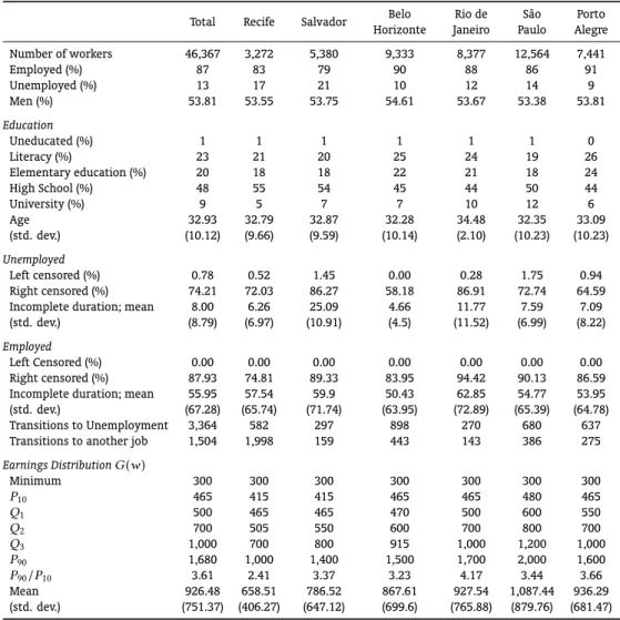
Table 5provides descriptive statistics regarding the final subsample. Included are some statistics related to demographic characteristics in order to provide an overview of the composition of each metropolitan market. All metropolitan areas have a male proportion between 53–54%. In terms of educational level, the structure is similar across regions, except for some differences. São Paulo has the largest proportion of workers with higher education, 12%, while in the metropolitan area of Recife, that proportion is only 5%. The mean age of workers is 33 years, and there is not a significant difference between regions.
Table 5.Descriptive statistics of subsample.
Total Recife Salvador HorizonteBelo JaneiroRio de PauloSão AlegrePorto
Number of workers 46,367 3,272 5,380 9,333 8,377 12,564 7,441
Employed (%) 87 83 79 90 88 86 91
Unemployed (%) 13 17 21 10 12 14 9
Men (%) 53.81 53.55 53.75 54.61 53.67 53.38 53.81
Education
Uneducated (%) 1 1 1 1 1 1 0
Literacy (%) 23 21 20 25 24 19 26
Elementary education (%) 20 18 18 22 21 18 24
High School (%) 48 55 54 45 44 50 44
University (%) 9 5 7 7 10 12 6
Age (std. dev.)
32.93 32.79 32.87 32.28 34.48 32.35 33.09
(10.12) (9.66) (9.59) (10.14) (2.10) (10.23) (10.23)
Unemployed
Left censored (%) 0.78 0.52 1.45 0.00 0.28 1.75 0.94
Right censored (%) 74.21 72.03 86.27 58.18 86.91 72.74 64.59
Incomplete duration; mean (std. dev.)
8.00 6.26 25.09 4.66 11.77 7.59 7.09
(8.79) (6.97) (10.91) (4.5) (11.52) (6.99) (8.22)
Employed
Left Censored (%) 0.00 0.00 0.00 0.00 0.00 0.00 0.00
Right censored (%) 87.93 74.81 89.33 83.95 94.42 90.13 86.59
Incomplete duration; mean (std. dev.)
55.95 57.54 59.9 50.43 62.85 54.77 53.95
(67.28) (65.74) (71.74) (63.95) (72.89) (65.39) (64.78)
Transitions to Unemployment 3,364 582 297 898 270 680 637
Transitions to another job 1,504 1,998 159 443 143 386 275
Earnings DistributionG(w)
Minimum 300 300 300 300 300 300 300
P10 465 415 415 465 465 480 465
Q1 500 465 465 470 500 600 550
Q2 700 505 550 600 700 800 700
Q3 1,000 700 800 915 1,000 1,200 1,000
P90 1,680 1,000 1,400 1,500 1,700 2,000 1,600
P90/P10 3.61 2.41 3.37 3.23 4.17 3.44 3.66
Mean (std. dev.)
926.48 658.51 786.52 867.61 927.54 1,087.44 936.29
(751.37) (406.27) (647.12) (699.6) (765.88) (879.76) (681.47)
4.66 months, and Rio de Janeiro has the largest, 11.77. For employed workers on the date of the first interview, the mean of employment duration (t1b+t1f) is 55.95 months. Rio de Janeiro has the highest mean, 62.85, while Belo Horizonte has the lowest, 50.43 months.
Regarding the wage distribution of employed workers on the date of the first interview, we observe a considerable difference between the metropolitan areas studied. The metropolitan region of São Paulo has the highest mean, R$1,087.44, and Recife has the lowest average, R$658.51, which represents only 60% of the state of São Paulo. Observing the ratio between the ninetieth and tenth percentiles, Recife also has a low-wage dispersion when compared to other metropolitan areas.
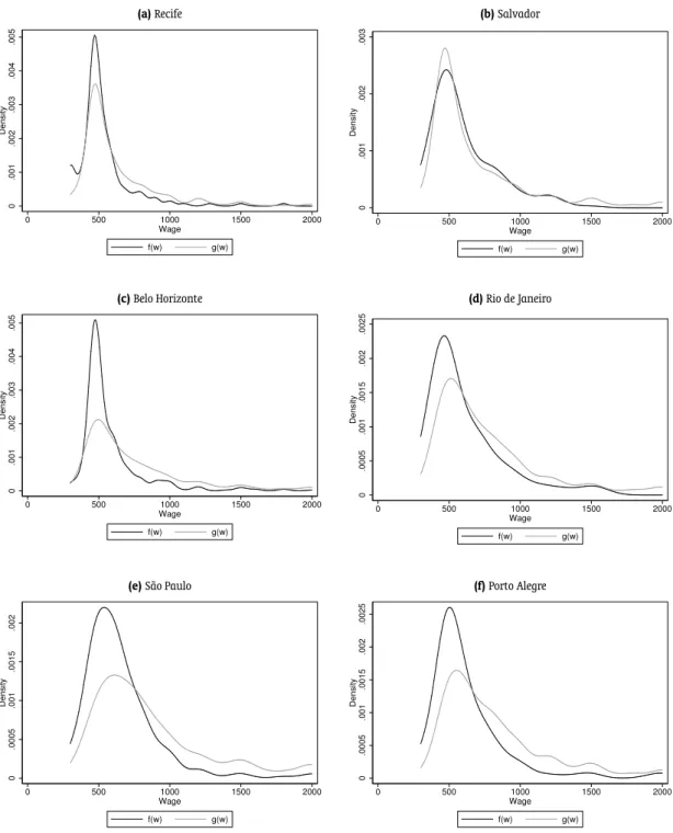
Finally,Figure 3shows kernel estimates of the density functions of the accepted wages distribution by workers who left the unemployment state during the survey, f(w) (wage offer distribution), and the wages distribution earned by workers who were employed at the date of the first interview,д(w)
(earnings distribution). Theory predicts that the wage offer distribution is dominated by the earnings distribution, due to the fact that the employed workers can migrate to jobs that pay higher wages. Referring toFigure 3, there is little difference between f(w) andд(w) for the metropolitan areas of
Recife and Salvador. However, for other regions, especially for São Paulo and Porto Alegre, there is a considerable difference between these distributions, which may be showing greater mobility of workers to jobs that pay better wages.
4.3. Structural Estimation
Job search models are usually estimated by maximum likelihood. In the case of the model in question, the wage offers distributionF(w)does not have an explicit form. Thus,Bontemps et al.(2000) proposed
a three-stage procedure to estimate the nonparametric model.
First, we need to specify the likelihood function. The model predicts that the unemployment duration is exponentially distributed with parameterλ0, due to the fact that the time between two events of a
Poisson process is exponentially distributed. The exponential distribution has the characteristic of being memoryless. Thus, this distribution has the property that the elapsed unemployment duration until the date of interview,t0b, and the residual unemployment duration(referring to remaining interviews),t0f, are independent and exponentially distributed10with parameter λ
0. The probability of sampling an
unemployed worker at the date of the first interview is equal to1/(1+k0)and if he/she receives a wage
offer,w0, this wage offer will be a realization ofF(·). Thus, we can write the likelihood function for an
unemployed worker as
Ld=λ 2−d0b−d0f
0
1+k0
exp[−λ0(t0b+t0f)]f(w0)(1−d0f), (22)
whered0b is equal to1ift0bis left censored, andd0f is equal to1ift0f is right censored.
The probability that an employed worker is observed is equal tok0/(1+k0)and the wage received
w1 is a realization of the earnings distribution, G(·). Job duration is exponentially distributed with
parameterθ, whereθ =δ+λ1F(w1), givenw1. The probability that a worker leaves the current job
to unemployment or to another job are equal toδ/(δ+λ1F(w1)) andλ1F(w1)/(δ+λ1F(w1)),
respec-tively. Again,t1b andt1f are the elapsed and residual job duration, respectively, and are assumed to be independent. The likelihood function for an employed worker is
Le=
k0
1+k0
д(w1)
(
δ+λ1F(w1)
)1−d1b exp
[
−(δ+λ1F(w1)
)
(t1b+t1f)
]
×
[
δv(λ1F(w1)
)1−v]1−d1f , (23)
whered1bis equal to1ift1bis left censored,d1f is equal to1ift1f is right censored, andvis equal to1 if the transition is to unemployment and0if it is to another job. Therefore, one can write the likelihood
Figure 3.Kernel estimates of wage distributions.
(a)Recife
0
.001
.002
.003
.004
.005
Density
0 500 1000 1500 2000
Wage f(w) g(w)
(b)Salvador
0
.001
.002
.003
Density
0 500 1000 1500 2000
Wage
f(w) g(w)
(c)Belo Horizonte
0
.001
.002
.003
.004
.005
Density
0 500 1000 1500 2000
Wage f(w) g(w)
(d)Rio de Janeiro
0
.0005
.001
.0015
.002
.0025
Density
0 500 1000 1500 2000
Wage
f(w) g(w)
(e)São Paulo
0
.0005
.001
.0015
.002
Density
0 500 1000 1500 2000
Wage
f(w) g(w)
(f)Porto Alegre
0
.0005
.001
.0015
.002
.0025
Density
0 500 1000 1500 2000
Wage
function for a sample of sizeN as
L=
N ∏
i=1
LdixLei(1−x), (24)
wherex is equal to1if the worker is unemployed at the time of the first interview and0if he/she is employed.
Moreover, using the relation betweenF(·) andΓ(·), we can generate the density function of firms’
productivities,γ(·). Thus, considering that the wage policy function11isw(p), the density function of firms’ productivity is
dΓ(p)
dp ≡γ(p)=f(w)w
′
(p). (25)
Using the inverse relationship withw(p), we can rewrite (25) as
γ(p)= f(w)
(w−1)′(w), (26)
where(w−1)′(w)
=∂w
−1(w)
∂w . Therefore, it becomes possible to obtain an expression forγ(p)for the two wage determination cases.
As already mentioned,F(w) does not have an explicit form, which makes the use of the likelihood
function alone impossible. Thus, we adopt the procedure proposed byBontemps et al.(2000). To esti-mate the bilateral bargaining model, we setρ=0. As it is also assumed inBurdett & Mortensen(1998)
in the wage posting model, due to the fact that this parameter cannot be identified from the data. We also setα=0.5andwDr=min{wi}Ni=1.
Note that by this procedure, the frictional parameters estimation (λ0,λ1 andδ), which is held in
the first two steps, is based only on worker’s behavior. Thus, it is expected that the estimatives of these parameters are consistent with different forms of firms’ behavior (Bontemps et al.,2000). Another important point is the fact that for the model not to be rejected by the data it must haveγ(p)>0. Then, from equation (26) wages and productivities must be positively related, which is a restriction generated by the theoretical model. For the estimation ofд(w), we use the Gaussian kernel function.
Finally, standard errors or confidence intervals ofλˆ0,λˆ1 andδˆ, are obtained using bootstrap repli-cations procedures, including the first stage. The bootstrap method is also useful to generate the confi-dence interval ofk1=λ1/δ, serving as an alternative to the delta method. The results follow.
5. RESULTS
This section presents the results of the structural estimation of the job search model. The results are divided into two sections. The first presents estimation results for the frictional parameters that are independent of the any wage setting behavior of firms. The second section presents the results for the estimated productivities distribution considering the two possibilities of wage determination.
5.1. Frictional Parameters
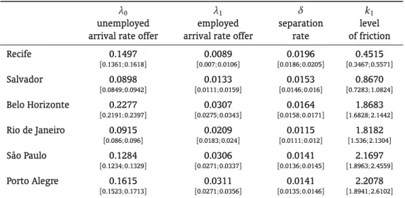
The frictional parameters are a measure of the search frictions present in the labor market that repre-sent the difficulty of workers and employers to establish working relationships. Table 6presents the estimatives for the six metropolitan areas that constitutes the PME.
First, the arrival rate of wage offers by unemployed workers,λ0, shows considerable heterogeneity
among the metropolitan areas studied. This rate in the metropolitan area of Belo Horizonte is 22.77%,
11In the case of wage posting models,w(p)≡K(p), and to the bilateral bargainw(p)
Table 6.Estimates of frictional parameters.
λ0
unemployed arrival rate offer
λ1
employed arrival rate offer
δ separation
rate
k1
level of friction
Recife 0.1497 0.0089 0.0196 0.4515
[0.1361;0.1618] [0.007;0.0106] [0.0186;0.0205] [0.3467;0.5571]
Salvador 0.0898 0.0133 0.0153 0.8670
[0.0849;0.0942] [0.0111;0.0159] [0.0146;0.016] [0.7283;1.0824]
Belo Horizonte 0.2277 0.0307 0.0164 1.8683
[0.2191;0.2397] [0.0275;0.0343] [0.0158;0.0171] [1.6828;2.1442]
Rio de Janeiro 0.0915 0.0209 0.0115 1.8182
[0.086;0.096] [0.0183;0.024] [0.0111;0.012] [1.536;2.1304]
São Paulo 0.1284 0.0306 0.0141 2.1697
[0.1234;0.1329] [0.0271;0.0337] [0.0136;0.0145] [1.8963;2.4559]
Porto Alegre 0.1615 0.0311 0.0141 2.2078
[0.1523;0.1713] [0.0271;0.0356] [0.0135;0.0146] [1.8941;2.6102]
Notes:2.5% and 97.5% percentiles of bootstrap distribution. 100 replications. Time unit: months.
while in Salvador this rate is only 8.98%, which implies an expected completed unemployment dura-tion12of approximately 11 months. This rate has a direct influence on unemployment rates, because the faster unemployed workers find jobs, the lower is the unemployment rate in the economy, given a level of destruction of employment relations (separation rate).
Compared to other studies, the estimated values ofλ0 in our paper are relatively higher. In
Bon-temps et al.(2000) this rate is on average 0.07 and inSulis(2008) this rate ranges between 0.04 to 0.07, but the author highlights the fact that the measure of unemployment duration used in the study is the time that the worker remains outside the administrative records used, which may be caused by unem-ployment, employment in public service, self-employment and inactivity. On the other hand, according toBontemps et al.(2000) the parameters estimated byKiefer & Neumann(1993) are two times higher than those estimated by the first authors, which would be closer to the values we have found here.
Regarding the arrival rate of wage offers for employed workers, λ1, we find that this rate is
con-siderably smaller thanλ0. This is in accordance with the international literature. Compared to other
metropolitan areas, Recife has a considerably low level of λ1, only 0.89%. São Paulo and Porto
Ale-gre have a rate approximately three times Ale-greater than Recife’s. This fact is already an indication that workers have greater mobility in these metropolitan areas, which implies higher competition among employers.
The separation rate is more homogeneous among the metropolitan areas. On average, approximately 1.5% of employed workers become unemployed per month. Rio de Janeiro has the lowest separation rate among the regions analyzed, indicating that the labor market in this region has a lower turnover. The results coming from the international literature are distinct. Van den Berg & Ridder (1998)and Bontemps et al.(2000) estimate a rate on average of 0.005 and 0.0061 for the Netherlands and France, respectively. On the other hand,Sulis(2008) estimated a rate of 0.0128 for Italy andBunzel et al.(2001) estimateδ between 0.01 to 0.02 for Denmark, which are closer to those estimated by us. Kyyrä(2007) found high values ofδ for Finland, estimatives ofδ in his work range from 0.05 to 0.01.
It is about the right place to deepen our analysis and try to connect our estimates with the prevalent regional inequalities in Brazilian labor markets described insection 2. We start by rationalizing regional
12As the duration of unemployment is assumed distributed exponentially with parameterλ
0, the expected full length is simply
inequalities on unemployment rates and the estimated deep parameters of our model, say,λ0,λ1andδ
onTable 6. Sinceδ is roughly homogenous, we focus on bothλ0andλ1. For instance, let us start with
Bahia, which presented in 2009, accordingly toTable 3, an unemployment rate of 11.37 and compare it to Porto Alegre (with a 5.42 unemployment rate). Do our structural estimates have a bite on that regional inequality? We think the answer is yes. While Salvador has the lowest rate of wage offer while unemployed (0.0898) and one of the lowest rate of wage offer while employed (0.013), ahead of Recife only, Porto Alegre has almost twice Salvador’s wage offer while unemployed (0.1615) and almost three times its rate of wage offer while employed (0.0311). So, no wonder Salvador and Porto Alegre occupy the extremes in terms of unemployment inequality in Brazil. More specifically, from an efficiency point of view any policy aiming improvements on Salvador’s unemployment rate must act on its very low arrival of wage offer while employed, something that has to do with its internal labor market.
If we want to draw a more regional explanation here, definitely we would look at the values of λ1, the arrival rate of wage offer while employed. The second column in6brings us an important
hint: metropolitan areas belonging to the South and Southeast regions have at least twice, sometimes three times, the correspondingλ1 of Recife and Salvador, both areas in the Northeast. In other words,
the scanty debate about regional differences in unemployment rate can be both backed up and, more importantly, can be deepened with our results, by noting that the inefficiency of internal labor markets in the Northeast is a driving force of that phenomena.
Fromλ1andδ one can obtaink1, which is a parameter of great importance in the model because
it is a measure of the level of friction in the labor market (van den Berg & van Vuuren,2003). This is becausek1 measures the number of expected job offers to be received by a worker during an episode
of employment, reflecting the level of competition among firms in the market. Hence, in a market that employed workers receive alternative offers at a higher rate, employers have incentives to offer better wages to reduce the outflow of workers. Besides this effect, of course, workers move more quickly into jobs that pay better wages, which implies that the earnings distribution,д(w), tends to dominate the wage offer distribution, f(w). Now, let us step into the regional inequality in wages appearing in Table 1.
The effect ofk1 on the distributions is evident atFigure 3(page87). It is observed that for the
metropolitan areas that have lowerk1 values, the distributions of f(w) andд(w) are closer, which is
the case of the metropolitan areas of Recife and Salvador. However, São Paulo and Porto Alegre have values ofk1, approximately four times higher than that of Recife and the effect is thatд(w)moves away
from f(w), i.e., workers have a faster wage growth in these regions. Thus, we got some evidence that
the higher the level of friction in the market (lowerk1) is, the more concentrated the wage distribution
is because workers have a low transition rate to jobs that pay better wages. Hence, our structural estimates corroborate past finds and, again, shed light on the debate: regional inequality in wages, besides being an outcome of its regional human capital distribution, can be rationalized as inequality of labor market search frictions.
How reasonable are our estimates? Table 7gives us some hints: it shows a comparison between our estimatives13and those estimated in other studies. The estimated value ofλ
0in our paper is
con-siderably higher than those on other studies, butCarvalho(2012) has a value close to that estimated in this study. As explained earlier, some authors make use of nonemployment durations, which include individuals who remained out of the workforce instead of using strictly unemployment duration data. Therefore, it is expected that the nonemployment duration mean be higher than the unemployment du-ration mean, which is calculated based on those workers who are actively seeking employment. There is also a chance of encountering a memory bias due to the fact that respondents underestimate the actual time they are searching for a job, which contribute to the estimation of high values ofλ0. As toλ1, our
estimatives are only slightly less than the estimated invan den Berg & Ridder(1998).
Table 7. Comparison of estimated values of frictional parameters.
Country λ0 λ1 δ k1
Our results Brazil – PME 0.129 0.022 0.015 1.467
Van den Berg & Ridder (1998) Netherlands 0.033 0.047 0.005 9.400
Bontemps et al.(2000) France 0.063 0.008 0.006 1.333
Bunzel et al.(2001) Denmark 0.028 0.010 0.015 0.235
Sulis(2008) Italy 0.043 0.006 0.013 0.462
Carvalho(2012) Brazil – PPV 0.137 0.005 0.005 1.000
By comparingk1, the value found here is close to the estimate for France byBontemps et al.(2000).
However, invan den Berg & Ridder(1998), the value ofk1 is estimated at about 9.40, which is
consid-erably high and the authors find a low level of monopsony power by firms. On the other hand,Sulis (2008) estimated a lowk1 which means high levels of monopsony power.
In the model with homogeneous firms, such asBurdett & Mortensen(1998), wage dispersion is caused only by search frictions. However, when we include heterogeneity in the firms’ productivity, the dispersion is also caused by differences of firms. The next section investigates the productivity distribution from the two possibilities of firms’ behavior assumed in this work and trace a parallel between that and regional differences in labor productivity.
5.2. Productivities Distribution
As we saw insection 2.3, the first decade of the 21st century witnesses a falling labor productivity all over Brazil. Here, we will try to give alternative explanations not for this decline but for the still prevalent regional differences in productivity. The productivity distribution is obtained from the third step of the estimation process (Bontemps et al.,2000). Such step is related to finding the productivity levels associated with observed wages in the sample, exploiting the first order conditions, given the frictional parameters estimated in previous steps. In addition, for each productivity level, we estimate the corresponding value of the density function,γ(p) associated to Γ(·) which is one of the model’s
primitive.
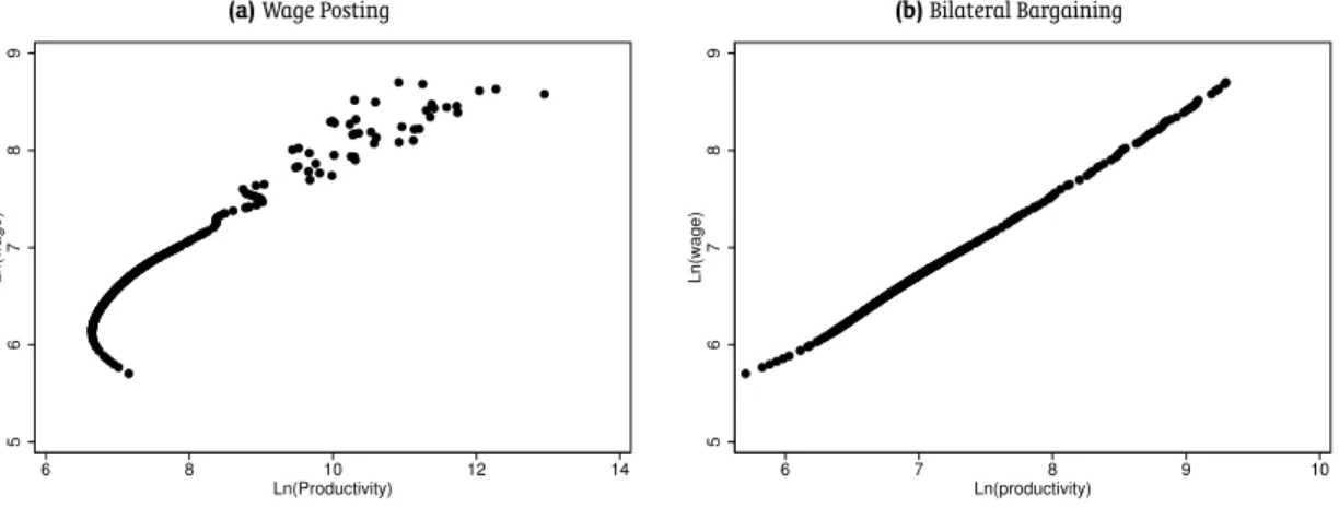
This step is performed for each possible wage determination analyzed: bilateral bargaining and wage posting. One of the restrictions shared by both wage determination mechanisms is to observe an increasing relationship between wages and productivities. This condition is satisfied for the bilateral bargaining case, but not wage posting. Mortensen(2003) finds the same result for the labor market in Denmark. This result14can be seen inFigure 4. In the wage posting case, the theory is rejected at lowest observed wages, where the relationship is decreasing, implying that those wages cannot be profits maximizing for firms. That is, the model does not explain the left tail of the wage distribution. The shape of the relationship between wages and productivity is similar to that found byMortensen (2003, p.103).
Besides the fact of not observing an increasing relationship between wages and productivity, the wage posting model generates implausible values for the firms’ productivity levels.Table 8shows the estimated productivity levels for the stock of employed workers on the date of the first interview. As the largest and most developed metropolis, it is expected that firms in São Paulo have the highest average productivity level. However, the metropolitan area of Recife has the highest average productivity level and after Recife, Salvador has the second highest. This may be due to the fact that estimated productivity
14It represents the relationship between wages and productivity for the metropolitan region of São Paulo. Other metropolitan
Figure 4.Relationship between wages e productivities.
(a)Wage Posting
5
6
7
8
9
Ln(wage)
6 8 10 12 14
Ln(Productivity)
(b)Bilateral Bargaining
5
6
7
8
9
Ln(wage)
6 7 8 9 10
Ln(productivity)
Table 8.Estimated productivities distribution: wage posting.
Minimum P10 Q1 Q2 Q3 P90 P90/P10 Mean
Recife 849.94 851.63 851.63 1,149.04 2,812.47 6,298.05 7.40 5,903.52
Salvador 730.30 748.52 748.52 1,109.06 2,308.59 8,190.00 10.94 5,350.19
Belo Horizonte 642.59 661.69 676.81 941.36 1,993.42 6,159.22 9.31 4,264.10
Rio de Janeiro 694.92 712.04 747.33 1,174.25 2,327.15 8,801.40 12.36 4,424.64
São Paulo 768.79 781.69 883.96 1,268.75 3,139.06 8,156.23 10.43 4,147.55
Porto Alegre 694.14 710.52 788.53 1,068.96 2,070.59 6,424.08 9.04 4,142.61
Note:P10,P90,Q1,Q2,Q3are percentiles e quartiles.
levels are too high for firms that pay the highest wages and are in the right tail of the distribution. Therefore, as the probability mass at the end of the distribution tends to zero, the estimated productivity level tends to be extremely high, inflating the mean. InFigure 3(on page87), we find that the density function of wages to Recife is closer to zero for higher wages than to São Paulo.
Shimer(2006) and Mortensen(2003) noted that the model with wage posting tends to estimate implausible productivity levels. Sulis(2008) also found high values for the estimated productivity and restricts its analysis to qualitative questions. Bontemps et al. (2000) argue that large differences in productivity and wages for some firms are due to the presence of the employer’s large capital stock, not treated in the model, which would generate a positive effect on labor productivity. Hence, from now on we stick to the bilateral bargaining model both on empirical grounds and on the Brazilian union structure described, for instance, inAmadeo(1994).
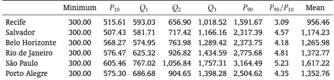
Table 9shows the estimated productivity distribution for employed workers, considering the case in which wages are determined as a result of a bilateral bargaining process. In this case, the metropolitan area of Recife has the lowest average productivity level, R$956.46. Now, São Paulo has, on average, the highest estimated labor productivity level, R$1,617.22, approximately 69% higher than Recife’s average. Note that the values are much smaller than those presented inTable 8. In terms of dispersion and considering the ratio between the ninetieth and tenth percentiles, São Paulo and Rio de Janeiro have the greatest productivity dispersion.