Rev. Bras. Econ. vol.68 número2

(1)

Exchange Rate Misalignments,

Interdependence, Crises, and Currency

Wars: An Empirical Assessment

∗

Emerson Fernandes Marçal

†

Contents: 1. Introduction; 2. Motivation; 3. Literature on exchange rate misalignment; 4. Econometric methodology; 5. Database description; 6. Results; 7. Comparison with the results of existing literature; 8. Conclusions; 9. Appendix A:;

10. Appendix B: Complementary Tables.

Keywords: Real effective exchange rate, Cointegration, Exchange rate misalignment JEL Code: E00; F31; C30.

This study aims to compare two different methodologies of calcula-ting exchange rate misalignment and test whether there is interdepen-dence among countries in determining the real effective exchange rate. Two different econometric approaches are used to achieve these go-als. The first one involves estimating a multivariate time series model that contains only country-specific variables and evaluating if this basic model can be improved by adding other countries’ variables. The study uses the algorithm suggested by Hendry and Krolzig (2005). to select the best model specification. The second strategy involves estimating long panel data with the real effective exchange rate and fundamentals for a group of countries and explicitly testing the interdependence hy-pothesis. The results suggest that the long-run exchange rate is mainly driven by its own fundamentals for most countries. The existence of interdependence is restricted to short-run dynamics.

Este trabalho tem por objetivo comparar metodologias distintas para cálculo de desalinhamento cambial além de testar a hipótese se as taxas de câmbio dos diversos países sofrem influencia apenas dos seus próprios fundamentos ou também da taxa de câmbio e dos fundamentos de outros países. Estas hipóteses consistem, respectivamente, na ausência ou na ex-istência de interdependência entre os diversos países. Para realizar tal tarefa utilizam-se duas estratégias empíricas. A primeira baseia-se em avaliar se

∗_{The author gratefully acknowledges financial support from BNDES and ANPEC. Any opinions expressed are those of the author}

and not those of BNDES and ANPEC.

(2)

244

Emerson Fernandes Marçal

um modelo multivariado de séries de tempo usualmente utilizada na liter-atura de desalinhamento cambial com dados apenas do próprio país em análise pode ser melhorado através da adição de variáveis relacionadas a outros países usando o algoritmo proposto por Hendry and Krolzig (2005). A segunda estratégia consiste em estimar um panel longo com as variáveis utilizadas para estimar desalinhamento cambial e testar formalmente a hipótese de ausência de interdependências. Os resultados sugerem que em ambas estratégias existe evidência de existência de interdependência. Esta ocorreria mais por conta de fatores ligados ao curto prazo, ou seja, o que explicaria o valor da taxa de câmbio de um país no longo prazo seriam seus próprios fundamentos enquanto no curto prazo fatores externos poderiam causar desvios.

1. INTRODUCTION

The exchange rate is an important macroeconomic variable and its variation affects global and sectorial economic activity, prices and interest rates, and trade flows. Large fluctuations of the exchange rate exacerbate debates regarding whether such movements are “excessive,” reflect “fundamentals,” or are “rational.”

Empirical literature on the exchange rate has advanced toward building models for assessing the long-term determinants of real exchange rates. Empirical strategies can be formulated based on models that use the doctrine of Purchasing Power Parity or an analysis based on fundamentals.1

Given this second approach, in this study, I estimate the long-term determinants of the real exchange rate of the G-20 as well as certain other selected countries. From these models, I construct the estimates of exchange rate misalignment for each country and test whether there is interdependence between various currency misalignments. The results suggest that the long-run exchange rate is mainly driven by its own fundamentals for most countries. The existence of interdependence is restricted to short-run dynamics.

The remainder of this paper is organized in the following manner. In the second section, I discuss the importance of exchange misalignment. In the third section, I conduct a non-exhaustive review of existing literature. In the fourth section, I discuss the econometric methodology employed in greater detail. In the fifth section, I present the results and compare them with those of similar studies in existing literature. In the last section, I present some conclusions.

2. MOTIVATION

The severity of the crisis in the US economy in 2008 brought the fear of a strong negative contagion in the rest of the world. Among other measures, the US authorities adopted an aggressive monetary policy with a strong reduction in nominal interest rates and monetary expansion. According to analysts, such measures generated strong pressure for US dollar depreciation against currencies of countries whose governments did not follow a similar monetary policy of lowering their domestic interest rates. If a country chooses not to follow such a reduction and opts to keep interest rates unchanged and accumulate reserves to prevent appreciation of its currency, it will eventually have to face inflation pressures. Some authors argue that the Federal Bank, after the sub-prime crisis, has been trying to use

1_{Clark and MacDonald (1998). Exchange rates and economic fundamentals: a methodological comparison of BEERs and FEERs,}

International Monetary Fund.

(3)

Exchange Rate Misalignments, Interdependence, Crises, and Currency Wars: An Empirical Assessment

monetary policy to generate a depreciation of the dollar rate to create an aggregate demand stimulus to speed up economic recovery. This policy has generated worldwide repercussions, and the possible disadvantages of such effects are a subject of debate.

One of the channels through which the monetary policy operates is real exchange rate depreciation. If the effect on other countries is deleterious, these countries could attempt to use available instruments to avoid the appreciation of their local currencies. This might configure a policy known in the literature as “beggar thy neighbor”.2_{Countries can adopt measures to prevent the appreciation of their currencies}

to avoid internalizing the costs of a deliberate expansionary monetary policy (“quantitative easing”).3 A cost-benefit analysis of this policy should be conducted not only for ascertaining its short-term effects but also for its long-term effect on output, inflation, and the welfare of countries. The countries’ strategic choice should aim to obtain short-term economic gains through an expansionary monetary policy despite being exposed to suffering some sort of retaliation from partners. It is also important to analyze the circumstances under which a country’s partners do not retaliate and accept the costs of appreciation as the best strategy.

For a small country, the strategy of attempting to retaliate is perhaps not the best as it is very difficult to cause significant damage to a leader country, thereby rendering such a policy ineffective. The main mechanism by which monetary policy would function is via devaluation of the exchange rate; however, for a small country, it would be difficult to counteract the effects of exchange rate appreciation by changing its own monetary policy. Turnovsky and Basar (1987) is an example of a study in which this strategic interaction is formally analyzed.

An expansionary monetary policy operates via the mechanism of excessive depreciation of currency. The degree and persistence of exchange rate misalignment is the mechanism by which net exports react in the short term and generate an increase in aggregate demand and smooth output fluctuations around its potential level. Some empirical questions can be formulated in this regard:

a) What is the extent to which monetary policy can generate a significant currency misalignment?

b) How long it will last?

c) Can significant misalignments of a country’s monetary policy be quickly offset by similar policies of relevant trading partners of the leader country?

d) What are the effects of such policies on the economic welfare of a country Turnovsky and Basar (1987)?

e) To what extent would the exchange rate policies of countries be the genesis of currency crises Glick and Rose (1998)?

3. LITERATURE ON EXCHANGE RATE MISALIGNMENT

The existing literature on the real exchange rate is vast. The classical doctrine and perhaps one of the oldest one is Purchasing Power Parity (PPP). Reference to this theory can be found in classical economics. Recently, some studies have collected evidence in favor of the validity of PPP for tradable goods, although the adjustment toward equilibrium can be very slow Froot and K. Rogoff (1995). Ahmad and Craighead (2010) analyzed monthly consumer price indexes for a secular American and British data set. The study showed strong evidence in favor of mean reversion, but with a high half-life. Their work follows Taylor’s guidelines Taylor (2001).

2_{Eichengreen and Sachs (1986). Exchange rates and economic recovery in the 1930s, National Bureau of Economic Research}

Cambridge, Mass., USA.

3_{Ugai (2007). “Effects of the quantitative easing policy: A survey of empirical analyses.” MONETARY AND ECONOMIC}

(4)

246 3.1. The economics of exchange rate misalignment

There is a theoretical discussion on the variables that drive the exchange rate in the long run. Two old but very important references are Edwards (1987) and Dornbusch (1976). The first analyzes economic misalignment, its causes, and consequences. The second is the classical model of flexible exchange rates. They analyze how monetary policy shocks can cause deviations from long-term PPP and the phenomena of under and over shooting.

Bilson (1979) and Mussa (1976) are also related classical studies. They are in keeping with the monetary approach to exchange rate. According to this approach, the exchange rate is linked primarily to the relative evolution of output and money supply among countries on the assumption that PPP and uncovered interest parity hold continuously and countries have stable money demand functions. However, Meese and Rogoff (1983) casts doubt on the explanatory power of this theory. The study showed that exchange rate forecasts that are constructed using this approach are not superior to a naive model such as a pure random walk with drift.

Stein (1995) proposes the natural rate of exchange approach (NATREX). According to the study, the equilibrium exchange rate level is determined at the point at which investment and savings generated by economic fundamentals are equal.

A classical reference to exchange rate misalignment is made by Williamson (1994). He defines equi-librium exchange rate as the level at which the country is able to maintain a certain desired level of deficit or surplus (seen as sustainable) in its external accounts. This is called the fundamental approach of the real exchange rate (FRER). Cline (2008) is another reference in this regard.

One source of criticism comes from the fact that there is a high degree of arbitrariness in choos-ing the desirable level of external accounts. Another source of criticism comes from the focus of the approach on flows and not on stocks.

Faruqee (1995) seeks to incorporate issues related to the evolution of stocks and builds a model in which there is an interaction between flows and stocks. Therefore, he shows that there must be a stable relationship between real exchange and the net foreign investment position between residents and non-residents. This is called the behavioral approach of the real exchange rate (BRER). The model was extended by Alberola and Cervero (1999). Further, Kubota (2009) developed a model with intertemporal consumption choice and capital accumulation. The model suggests that the real exchange rate is a function of relative terms of trade, net external position, and relative productivity of tradable and non-tradable sectors. This is the approach used in the current study.

The advantage of this approach is the low degree of subjectivity in the exchange rate misalignment estimate. The model connects the level of real exchange rate to a group of fundamentals obtained from a theoretical model. This approach is empirically implemented using an econometric model to decompose the series of real exchange rates into permanent and transitory components.

4. ECONOMETRIC METHODOLOGY

In this study, we propose to test whether the models estimated using a traditional approach to calculate currency misalignment from a list of fundamentals can be improved upon by modeling with long panel data that take into account a possible interdependence among different countries. In order to this, two testing strategies are used.

4.1. Testing Strategies

4.1.1. Strategy 1

The starting point is Larsson and Lyhagen’s model Larsson and Lyhagen (2007). It is a generalization of Johansen and Juselius’ procedure (Johansen (1988), Johansen (1995) and Juselius (2009)).

(5)

Letxit = [RERit F undamentalsit] be the vector that contains the real exchange rate and its

fundamentals at time t for countryi, and letXt= [x′lt...x′N t]′be the vector in which country data are

stacked.

The general model is given by the following equation:

∆Xt= Γ1∆Xt−1+...+ Γk∆Xt−k+ ΦDt+ABXt−1+εt (1)

whereεtrepresents random errors, andΩis its variance and covariance matrix of the shocks. Shocks

are assumed to be uncorrelated in time and cross-sectional dimensions. The vectorXt contains the

data series from all countries,Dtcontains deterministic terms, andθ= Γ1,...,Γk,Φ, A, Bdenotes the

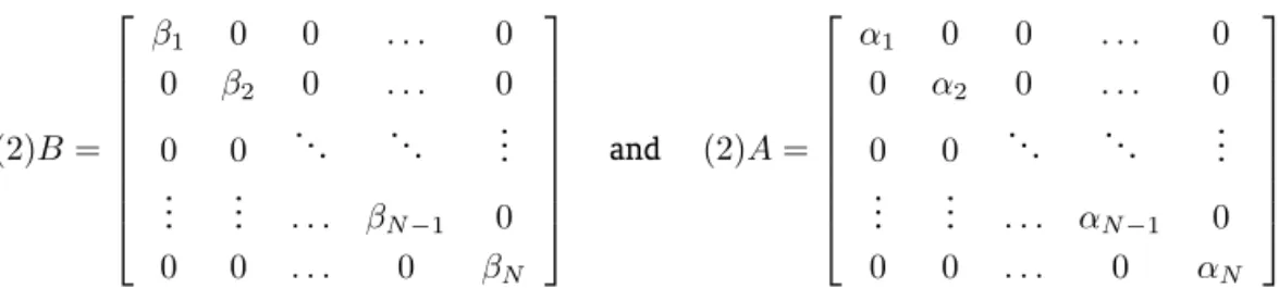
set of parameters to be estimated. In the general case, all the variables could cointegrate with each other,4_{but Larsson and Lyhagen (2007), for example, restrict their analysis to the case in which there}

can be cointegration only between variables of the same country. Then,

B=

        

β1 0 0 . . . 0

0 β2 0 . . . 0

0 0 . .. . .. ... ..

. ... . . . βN−1 0

0 0 . . . 0 βN

        

, (2)

whereβis a vector of dimensionpxri.

The matrix of load(A)has dimension(P XN)x(r1 +r2 + +rN)and noa prioriconstraint and enables all sorts of configuration, provided that the system is stable. One cointegrated vector that contains the variables of one country can generate not only part of the equation of that country but also other countries’ equations. It is precisely this possibility that makes this structure attractive for analyzing the problem considered in this work.

For example, it is possible to test if the cointegration vector, which represents the fundamentals of a country (e.g., US), is present in exchange rates and fundamentals variables’ equations. This hypothesis could be tested under the null hypothesis that certain elements of matrixAare zero. Larsson and Lyha-gen (2007) showed that after the rank of a long-run matrix is determined, the test can be implemented using a likelihood ratio test with an asymptotic chi-squared distribution. The authors also derived a test to determine the rank of cointegration; this test has no standard asymptotic distribution, and this distribution was tabulated. Among other interesting hypotheses, it is also possible to test jointly, for example, whether the net external investment position is one of the fundamentals for all analyzed countries.

One limitation of this structure is the untested assumption thatB is a diagonal matrix. Except for cases in which the temporal dimension of the database is sufficiently large, it is difficult to assess the validity of this hypothesis due to the curse of dimensionality. In order to circumvent this problem, we chose two different strategies. We estimated models with small sizes in relation to time and cross-sectional dimensions. We decided to estimate models for all combinations of countries taken as pairs for a sample with data from 1981 to 2011, and a model of higher dimension with five developed countries and Brazil using a larger sample (beginning in 1970).

The estimation of the model is done by using the algorithm of generalized reduced rank regression (GRRR) developed by Hansen (2003). All restrictions imposed on the general model can be tested using a likelihood ratio test with an asymptotic chi-squared distribution.

4_{The concept of cointegration has become widely used in empirical research with the seminal work of Engle e Granger (1987).}

(6)

248

The likelihood ratio procedure used in the study suffers from a serious size distortion. This encour-ages analysts to use a bootstrap technique to obtain appropriate critical values. Studies that discuss similar problems are Johansen (1999), Johansen et alii (2000), Gredenhoff and Jacobson (2001), and Swensen (2006). We chose to perform a bootstrap to simulate the appropriate distribution for the test statistic. The results suggest that the size distortion is actually severe.

4.1.2. Strategy 2

The second strategy for testing the existence of interdependence involves estimating multivariate models. First, a country-by-country analysis is done to obtain the long-term relationships that will be used as input for the construction of the exchange rate misalignment estimate. Then, the error correc-tion mechanisms obtained for all countries are included in each individual country model. Thereafter, their relevance is tested using the algorithm suggested by Santos and Hendry (2008) and Hendry and Krolzig (2005). This procedure was implemented using software Oxmetrics. If the final selected model contains only the series of the individual country, it can be concluded that there is no evidence for the interdependence hypothesis, whereas in the event that the final country model contains variables related to other countries, it can be concluded that there is some degree of interdependence.

4.2. Gonzalo and Granger’s decomposition

Many decomposition methods have been suggested for the decomposition of the process between permanent and transitory components.

The data generating process for a specific country is assumed to be a multivariate VECM model given by:

∆xit=ψi1∆xi,t−1+...+ψi1∆xi,t−k+1+φildit+αiβxi,t−1+vi,t (3)

wherevi,trepresents random errors, andθiis its variance and covariance matrix of the shocks. Shocks

are assumed to be uncorrelated in time. The vectorxi,t contains the data series for country i,di,t

contains deterministic terms, andθi =ψi1,..., ψi1,φi1,αi,βidenotes the set of parameters to be

esti-mated.

In general, the decomposition has the following form:5

xi,t=βi,⊥(c′βi,⊥)−

1

c′xi,t+c⊥(βi′c⊥)−

1

βi′xi,t (4)

The decompositions vary according the choice of vector c. A condition for the existence of the decomposition is that the matrix(β′

ic⊥)has full rank. However, this condition is not always satisfied.

Gonzalo and Granger (1995) propose thatc=αi,⊥.6This representation always exists for the case

of a VECM of zero order. Johansen (1995) proposes that . This decomposition exists in the system since there are variables whose order of integration is at most 1. Kasa (1992) proposes that . Another possibility is to generate forecasts from the VECM estimated for each point. The values for which the series converge are the fundamentals. In this study, I use the decomposition given by Gonzalo and Granger (1995).7

5_β_⊥_{denotes the vector orthogonal to}_β_{in such a manner that}_β′_⊥_β_{= 0}

6_{Gonzalo and Granger’s decomposition-Gonzalo, J. and C. W. J. Granger (1995). “Estimation of Common Long-Memory}

Compo-nents in Cointegrated Systems.” Journal of business and Economics Statistics 13(1).was implemented in Matlab software.

7_{In this case, the components of the deterministic model as constant and time trends should be restricted to the space of}

cointegration.

(7)

In Gonzalo and Granger’s decomposition, there is no Granger causality between transitory and permanent components in that the former do not8 _{cause a change in permanent components in the}

long run; in other words, the exchange rate misalignment, defined as the transitory component of the real exchange rate equation in a multivariate system, does not contain information that is relevant for predicting the change in the permanent components in the long run.9 _{Gonzalo and Granger’s}

decom-position is widely used in the literature of exchange rate misalignment. See, for example, Alberola and Cervero (1999). Their decomposition can be easily adapted if the data generating process is given by (1).

5. DATABASE DESCRIPTION

The data for this study were collected from the International Financial Statistics of the International Monetary Fund (IMF). The real exchange rate for each country is calculated from a basket of currencies that uses data from consumer price indexes. The data on net foreign investment position and reserves have been collected by the IMF from 2000 onward and those for previous years were collected on the basis of those given in Lane and Milesi-Ferretti (2007). The gross domestic product data were collected from the World Bank World Development Indicators available online.

The codes were run in Matlab and Oxmetrics software, and the frequency is annual. In many cases, data begins in 1970 and ends in 2010; in other cases, the sample begins in 1980 and ends in 2010. The countries that are analyzed are Australia, Brazil, Canada, Colombia, Denmark, Finland, France, Germany, Greece, India, Italy, Portugal, Ireland, Japan, Mexico, Netherlands, South Korea, South Africa, Singapore, Spain, Sweden, United Kingdom, Uruguay, Turkey, and the United States. Data from 1970 until 2012 is not available for all countries. However, all listed countries at least have information from 1980 onward.

6. RESULTS

As a first step, analysis tests were conducted using multivariate cointegration Johansen (1988). For countries that showed significant relationships, the error correction mechanisms were calculated. Table 20 contains the results of cointegration tests Johansen (1988), Shin (1994), and Engle e Granger (1987). The estimated error correction mechanism was used as input for strategy 2. Moreover, the error correction mechanisms were again estimated for strategy 1.

6.1. Results of Strategy 1

6.1.1. Long panel data (1970-2010): Australia, Brazil, Canada, the United States, Japan, and the United Kingdom

In order to investigate the existence of interdependence among exchange rate misalignments in the above countries, I estimated the model of equation (1). The model under the null hypothesis is given by

8_{For a rigorous definition of Granger causality, see Hendry (Hendry (1995). Dynamic Econometrics. Oxford, Oxford University}

Press).

9_{If the most appropriate VECM contains only the erroneous mechanism and deterministic terms, then Gonzalo and Granger’s}

(8)

250

(2)B=

        

β1 0 0 . . . 0

0 β2 0 . . . 0

0 0 . .. . .. ... ..

. ... . . . βN−1 0

0 0 . . . 0 βN

        

and (2)A=

        

α1 0 0 . . . 0

0 α2 0 . . . 0

0 0 . .. . .. ... ..

. ... . . . αN−1 0

0 0 . . . 0 αN

        

Except for the variance and covariance matrices of the shocks, there is no source of interdependence. In the alternative hypothesis, matrices A and B are completely unrestricted.

The results of this test are presented in Table 1. Based on the asymptotic value, the null hypothesis is easily rejected, but it is accepted if bootstrap critical values are used. Since the tests can suffer from size distortions, I tend to rely on the option of not rejecting the null.

Table 1: Results of the test for assessing the existence of interdependence based on misalignments in exchange rates

Likelihood Ratio Test:

Test Statistic 689,67

Number of restrictions 180

asymptoticalp-value 0,00%

bootstrap p-value* 28,10%

* 300 replications.

6.1.2. Peer analysis: Using data from 1980-2011 andN = 2

The second group of estimates was conducted using pairs of countries. The results are presented in Table 2. Again, the difference between the asymptotic critical and simulated critical values is large. As a general rule, the simulated critical values were consistently larger than the asymptotic critical values. The analysis in Table 2 suggests that there is an important interdependence across countries, and these findings are not in line with the evidence presented in section 6.1.1. For example, in the Brazilian case, there is evidence of interdependence with the United Kingdom, the United States, and Australia. The lack of interdependence between Brazil and Canada as well as Canada and Japan is confirmed. Interdependence was detected for the United States with Brazil, Canada, France, India, South Africa, South Korea, and the United Kingdom. However, there is no evidence of interdependence between the remaining countries and the United States. Further, there is strong evidence of interdependence among European countries, as expected.

(9)

Ex change Rate Misalignments, Inter dependence, Crises, and Curr ency W ars: An Empirical Assessment

Table 2: Dependence tests with models from pairs of countries: Short Panel

Australia Brazil canada Colombia Denmark finland france germany Greece India Ireland Japan Mexico Netherlands South Korea South Africa Singapore Spain Sweden UK Uruguay United States Austria Statistic 38,9 43,4 23,4 25,3 27,5 31,4 32,0 29,1 42,6 34,2 33,7 52,8 25,4 55,1 26,9 31,9 46,9 62,1 24,2 29,9 29,3 29,8

Asymptotic p-value 0,0% 0,0% 0,9% 0,5% 0,2% 0,1% 0,0% 0,1% 0,0% 0,0% 0,0% 0,0% 0,5% 0,0% 0,3% 0,0% 0,0% 0,0% 0,7% 0,1% 0,1% 0,1% Boostrap p-value 8,0% 4,0% 22,0% 48,0% 54,0% 30,0% 28,0% 36,0% 24,0% 10,0% 18,0% 0,0% 44,4% 4,0% 48,0% 22,0% 2,0% 8,0% 36,0% 18,0% 38,0% 46,0% Australia Statistic 58,9 47,0 36,4 40,6 44,8 13,1 21,8 18,9 34,0 21,8 24,0 31,8 24,2 23,6 40,6 33,4 22,5 35,3 29,9 16,5

Asymptotic p-value 0,0% 0,0% 0,0% 0,0% 0,0% 22,0% 1,6% 4,1% 0,0% 100,0% 1,6% 0,8% 0,0% 0,7% 0,9% 0,0% 0,0% 1,3% 0,0% 0,1% 8,6% Boostrap p-value 0,0% 6,0% 2,0% 10,0% 0,0% 42,0% 12,0% 60,0% 2,0% 38,0% 20,0% 2,0% 6,0% 24,0% 0,0% 4,0% 48,0% 2,0% 26,0% 46,0% Brazil Statistic 24,2 23,6 31,3 11,2 21,7 40,7 22,9 18,3 33,8 27,5 21,6 24,7 16,9 26,9 41,3 22,1 10,6 49,0 27,5 42,4

Asymptotic p-value 0,7% 0,9% 0,1% 34,4% 1,7% 0,0% 1,1% 4,9% 0,0% 0,2% 1,7% 0,6% 7,7% 0,3% 0,0% 1,5% 38,8% 0,0% 0,2% 0,0% Boostrap p-value 14,0% 52,0% 18,0% 68,0% 30,0% 12,0% 56,0% 64,0% 34,0% 30,0% 24,0% 14,0% 44,0% 14,0% 2,0% 56,0% 84,0% 4,0% 6,0% 2,0% canada Statistic 39,3 21,7 48,7 45,8 32,8 23,8 39,0 23,5 15,7 24,7 44,0 12,5 25,8 19,4 22,1 21,1 28,9 21,4 31,0 Asymptotic p-value 0,0% 1,7% 0,0% 0,0% 0,0% 0,8% 0,0% 0,9% 10,9% 0,6% 0,0% 25,4% 0,4% 3,6% 1,4% 2,0% 0,1% 1,9% 0,1% Boostrap p-value 10,0% 32,0% 0,0% 0,0% 16,0% 32,0% 0,0% 38,0% 70,0% 4,0% 2,0% 60,0% 12,0% 50,0% 26,0% 18,0% 28,0% 42,0% 4,0% Colombia Statistic 28,2 36,9 32,5 36,7 39,2 20,3 26,2 31,5 32,8 36,7 19,2 87,2 33,5 46,4 21,9 36,2 29,9 34,2 Asymptotic p-value 0,2% 0,0% 0,0% 0,0% 0,0% 2,6% 0,3% 0,0% 0,0% 0,0% 3,8% 0,0% 0,0% 0,0% 1,5% 0,0% 0,1% 0,0% Boostrap p-value 16,0% 0,0% 8,0% 12,0% 12,0% 24,0% 20,0% 22,0% 2,0% 12,0% 26,0% 0,0% 0,0% 0,0% 28,0% 6,0% 18,0% 8,0% Denmark Statistic 29,8 25,2 29,9 46,2 25,8 34,7 48,2 22,9 37,8 47,1 44,8 49,6 53,5 38,3 31,9 26,5 41,2 Asymptotic p-value 0,1% 0,5% 0,1% 0,0% 0,4% 0,0% 0,0% 1,1% 0,0% 0,0% 0,0% 0,0% 0,0% 0,0% 0,0% 0,3% 0,0% Boostrap p-value 28,0% 44,0% 24,0% 26,0% 52,0% 46,0% 12,0% 48,0% 24,0% 8,0% 6,0% 2,0% 6,0% 6,0% 26,0% 52,0% 22,0% finland Statistic 47,7 24,8 53,7 56,6 35,9 45,1 23,8 26,4 26,7 39,5 30,6 43,6 41,3 24,5 28,1 36,5

Asymptotic p-value 0,0% 0,6% 0,0% 0,0% 0,0% 0,0% 0,8% 0,3% 0,3% 0,0% 0,1% 0,0% 0,0% 0,6% 0,2% 0,0% Boostrap p-value 2,0% 26,0% 6,0% 0,0% 26,0% 10,0% 62,0% 46,0% 38,0% 10,0% 32,0% 6,0% 14,0% 78,0% 34,0% 18,0% france Statistic 28,2 18,2 27,9 21,6 50,9 38,9 18,4 24,3 26,1 16,9 52,9 35,5 38,9 24,3 53,4

Asymptotic p-value 0,2% 5,1% 0,2% 1,7% 0,0% 0,0% 4,9% 0,7% 0,4% 7,8% 0,0% 0,0% 0,0% 0,7% 0,0% Boostrap p-value 16% 84% 56,0% 36,0% 4,0% 4,0% 64,0% 64,0% 28,0% 70,0% 0,0% 8,0% 12,0% 50,0% 4,0% germany Statistic 42,7 55,1 38,1 38,3 48,3 40,8 35,1 16,1 26,6 32,7 33,8 30,0 45,8 41,2 Asymptotic p-value 0,0% 0,0% 0,0% 0,0% 0,0% 0,0% 0,0% 9,7% 0,3% 0,0% 0,0% 0,1% 0,0% 0,0% Boostrap p-value 12,0% 2,0% 28,0% 24,0% 0,0% 8,0% 8,0% 72,0% 34,0% 8,0% 14,0% 38,0% 2,0% 16,0% Greece Statistic 33,9 57,5 32,7 44,9 39,9 36,0 34,2 36,0 67,5 35,3 45,7 39,4 41,3

Asymptotic p-value 0,0% 0,0% 0,0% 0,0% 0,0% 0,0% 0,0% 0,0% 0,0% 0,0% 0,0% 0,0% 0,0% Boostrap p-value 44,0% 4,0% 64,0% 40,0% 20,0% 16,0% 48,0% 28,0% 0,0% 22,0% 16,0% 30,0% 22,0%

India Statistic 42,2 28,5 27,0 76,7 45,8 45,8 53,9 30,2 54,6 40,5 71,6

Asymptotic p-value 0,0% 0,1% 0,3% 0,0% 0,0% 100,0% 0,0% 0,0% 0,1% 0,0% 0,0% 0,0% Boostrap p-value 18,0% 30,0% 60,0% 2,0% 20,0% 20,0% 4,0% 62,0% 0,0% 10,0% 0,0%

Ireland Statistic 31,6 27,6 19,1 21,1 36,6 26,7 31,9 33,4 54,1 41,8 22,9

Asymptotic p-value 0,0% 0,2% 3,9% 2,0% 0,0% 0,3% 0,0% 0,0% 0,0% 0,0% 1,1%

Boostrap p-value 40,0% 52,0% 68,0% 62,0% 20,0% 56,0% 26,0% 24,0% 2,0% 18,0% 30,0%

Japan Statistic 28,5 27,0 27,0 76,7 44,5 44,5 31,9 40,7 47,5 45,1

Asymptotic p-value 0,1% 0,3% 0,3% 0,0% 0,0% 0,0% 0,0% 0,0% 0,0% 0,0%

Boostrap p-value 48,0% 60,0% 54,0% 2,0% 6,0% 18,0% 34,0% 20,0% 18,0% 2,0%

Mexico Statistic 25,4 32,0 33,9 51,9 33,6 34,5 23,8 33,6 47,5

Asymptotic p-value 0,5% 0,0% 0,0% 0,0% 0,0% 0,0% 0,8% 0,0% 0,0%

Boostrap p-value 40,0% 14,0% 24,0% 2,0% 24,0% 12,0% 46,0% 46,0% 12,0%

Netherlands Statistic 44,7 36,1 36,5 46,6 19,7 42,5 30,3 44,7

Asymptotic p-value 0,0% 0,0% 0,0% 0,0% 3,2% 0,0% 0,1% 0,0%

Boostrap p-value 12,0% 12,0% 8,0% 4,0% 58,0% 2,0% 38,0% 12,0%

Continued on Next Page. . .

(10)

252

Emerson

Fernandes

Mar

çal

Table 2 – Continued

Australia Brazil canada Colombia Denmark finland france germany Greece India Ireland Japan Mexico Netherlands South Korea South Africa Singapore Spain Sweden UK Uruguay United States

South Korea Statistic 30,5 58,7 37,7 36,4 34,6 36,7 38,2

Asymptotic p-value 0,1% 0,0% 0,0% 0,0% 0,0% 0,0% 0,0%

Boostrap p-value 46,0% 0,0% 6,0% 2,0% 18,0% 2,0% 2,0%

South Africa Statistic 54,1 59,4 32,7 33,4 34,2 44,7

Asymptotic p-value 0,0% 0,0% 0,0% 0,0% 0,0% 0,0%

Boostrap p-value 2,0% 0,0% 16,0% 34,0% 30,0% 4,0%

Singapore Statistic 26,9 52,2 29,7 29,2 49,5

Asymptotic p-value 0,3% 0,0% 0,1% 0,1% 0,0%

Boostrap p-value 46,0% 0,0% 48,0% 46,0% 8,0%

Spain Statistic 30,6 44,5 43,3 26,3

Asymptotic p-value 0,1% 0,0% 0,0% 0,3%

Boostrap p-value 8,0% 2,0% 8,0% 66,0%

Sweden Statistic 35,0 32,8 29,9

Asymptotic p-value 0,0% 0,0% 0,1%

Boostrap p-value 78,0% 14,0% 88,0%

UK Statistic 24,9 54,3

Asymptotic p-value 0,6% 0,0%

Boostrap p-value 66,0% 0,0%

Uruguay Statistic 43,5

Asymptotic p-value 0,0%

Boostrap p-value 14,0%

RBE

Rio

de

Janeiro

v.

68

n.

2

/

p.

243–276

Abr

-Jun

(11)

6.2. Results of Strategy 2

The results of a sequence of tests for assessing the existence of interdependence among different countries are reported in the following tables. Two models are estimated. The first one is a multivariate VECM model for each country, expanded with the cointegration vectors of the remaining countries. Thereafter, I used a simplification algorithm available at Oxmetrics. The second model is a multivariate model that is expanded not only with the error correction mechanisms but also with the first difference of the logarithm of the exchange rate and the ratio of Net Foreign Asset Position (NFA) on GDP, which is the indicator of the Balassa-Samuelson effect. In this case, this second option not only tests the existence of interdependence of misalignments (imbalances) but also tests the short-run dynamics of a specific country in relation to the short-run dynamics of other countries.

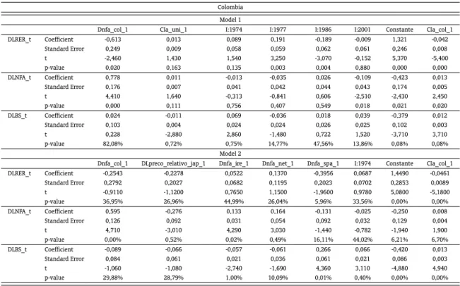
6.2.1. Brazil

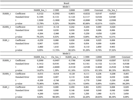
Table 3 presents the results of the multivariate model for Brazil. In the analysis of the extended model (model 1) using the cointegration vectors of other countries, The algorithm excluded the vari-ables of the Brazilian final model. Thus, the exchange rate misalignments elsewhere do not appear to cause large influences on the dynamics of the Brazilian series. The results from the search algorithm for outliers suggest three points of instability of the Brazilian model in 1999, 2008, and 2009. The last two are related to the recent developments of the international crisis. The first is related to the transition from an almost fixed exchange rate regime after the Real Plan to a floating exchange rate regime in 1999.

Table 3: Final model selected using the Ox algorithm: Brazil

Brazil Model 1

DLRER_bra_1 I:1999 I:2008 I:2009 Constant CIa_bra_1 DLRER_t Coefficient 0,2122 -0,3592 0,0651 -0,0232 0,0147 -0,0527

Standard Error 0,1395 0,1131 0,1125 0,1117 0,0184 0,0180 t 1,5200 -3,1800 0,5780 -0,2080 0,7990 -2,9300 p-value 13,78% 0,32% 56,69% 83,66% 43,01% 0,62% DLNFA_t Coefficient -0,013 -0,118 0,242 -0,204 0,000 -0,020 Standard Error 0,049 0,039 0,039 0,039 0,006 0,006 t -0,264 -2,980 6,180 -5,250 -0,050 -3,200 p-value 79,33% 0,53% 0,00% 0,00% 96,07% 0,31% DLBS_t Coefficient -0,259 0,088 0,028 -0,006 0,025 0,008 Standard Error 0,067 0,055 0,054 0,054 0,009 0,009

t -3,860 1,610 0,525 -0,110 2,850 0,903

p-value 0,05% 11,72% 60,32% 91,29% 0,74% 37,32% Model 2

DLRER_bra_1 CIa_bra_1 DLRER_usa_1 I:1999 I:2008 I:2009 Constant DLRER_t Coefficient 0,2090 -0,0497 -0,1766 -0,3490 0,0558 -0,0287 0,0132

Standard Error 0,1412 0,0191 0,3445 0,1161 0,1152 0,1134 0,0188 t 1,4800 -2,6000 -0,5130 -3,0100 0,4840 -0,2530 0,7040 p-value 14,87% 1,39% 61,16% 0,51% 63,16% 80,19% 48,63% DLNFA_t Coefficient -0,015 -0,018 -0,120 -0,111 0,236 -0,208 -0,001 Standard Error 0,049 0,007 0,119 0,040 0,040 0,039 0,006 t -0,309 -2,740 -1,010 -2,770 5,940 -5,320 -0,200 p-value 75,96% 0,99% 32,11% 0,94% 0,00% 0,00% 84,29% DLBS_t Coefficient -0,251 0,000 0,459 0,061 0,053 0,008 0,029

Standard Error 0,060 0,008 0,146 0,049 0,049 0,048 0,008

t -4,200 0,018 3,150 1,250 1,080 0,173 3,650

p-value 0,02% 98,58% 0,35% 22,20% 28,83% 86,39% 0,09%

(12)

254

Model 2 was obtained from the general model that contained not only the cointegration vectors of all the countries analyzed, but also the first difference from the logarithm of the variables collected for all countries. The final model suggests that the changes in the effective exchange rate in the United States influence the Brazilian economy. Either way, the dynamics of the Brazilian exchange rate do not appear to have been influenced directly by global factors. The only economy that appears to have influenced the Brazilian data is the US economy, and this was widely expected given the extent of trade and financial integration between the two countries.

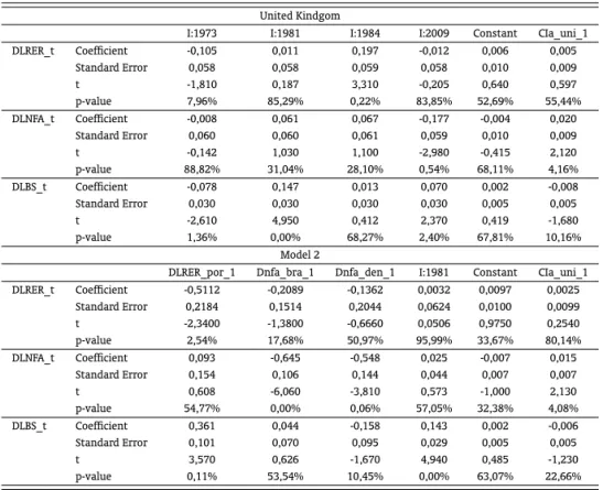
6.2.2. The United States

Table 5 presents the results of the tests of interdependence applied to the United States. The results suggest that the misalignment of other countries does not influence the dynamics of the model that contains US series. This result contrasts with the conclusions reported in section 6.1.2. Only the model with an extended information set provides evidence in favor of interdependence. The change in the real exchange rate of the Netherlands appears to be linked to United States data. This result is not intuitive and could have been due to the casual retention of unimportant variables. The results for the United States suggest that the US economy is barely influenced by changes in the economies of the rest of the world.

In the North American model, there were some points of instability-the years 1974, 1986, 2005, 2008, and 2009. The last two are associated with the recent financial crisis, while the first one is related to the oil crisis.

Table 4: Final model obtained from the selection made using the Ox algorithm: United States

United States Model 1

DLRER_usa_1 I:1974 I:1986 I:2005 I:2008 I:2009 Constant CIa_eua_1 DLRER_t Coefficient 0,5442 0,0502 -0,1537 0,0146 -0,0201 0,0513 -0,2004 0,0121757 Standard Error 0,1269 0,0446 0,0469 0,0429 0,0431 0,0436 0,1036 0,006329 t 4,2900 1,1300 -3,2800 0,3390 -0,4660 1,1800 -1,9300 1,92 p-value 0,02% 26,89% 0,26% 73,68% 64,48% 24,85% 6,22% 0,0636 DLNFA_t Coefficient -0,011 -0,014 0,011 0,078 -0,095 0,061 -0,043 0,002

Standard Error 0,070 0,025 0,026 0,024 0,024 0,024 0,057 0,003 t -0,152 -0,551 0,423 3,270 -3,980 2,530 -0,744 0,626 p-value 87,98% 58,53% 67,50% 0,26% 0,04% 1,68% 46,24% 53,62% DLBS_t Coefficient -0,175 0,358 0,109 0,038 0,020 -0,060 -0,203 0,012

Standard Error 0,151 0,053 0,056 0,051 0,051 0,052 0,124 0,008 t -1,150 6,720 1,950 0,745 0,386 -1,150 -1,640 1,550 p-value 25,75% 0,00% 5,98% 46,21% 70,20% 26,01% 11,04% 13,24%

Model 2

DLRER_net_1 I:1974 I:1986 I:2008 Constant CIa_eua_1 DLRER_t Coefficient -0,9557 0,0370 -0,1691 -0,0418 -0,1534 0,0095

Standard Error 0,2112 0,0424 0,0458 0,0413 0,0986 0,0060 t -4,5300 0,8720 -3,7000 -1,0100 -1,5600 1,5900 p-value 0,01% 38,92% 0,08% 31,91% 12,93% 12,18% DLNFA_t Coefficient 0,301 -0,026 0,022 -0,100 -0,076 0,004

Standard Error 0,136 0,027 0,029 0,027 0,064 0,004 t 2,210 -0,939 0,749 -3,760 -1,200 1,140 p-value 3,39% 35,47% 45,89% 0,07% 23,73% 26,30% DLBS_t Coefficient 0,085 0,368 0,103 0,028 -0,188 0,011

Standard Error 0,265 0,053 0,057 0,052 0,124 0,008 t 0,322 6,920 1,790 0,548 -1,520 1,430 p-value 74,96% 0,00% 8,31% 58,75% 13,75% 16,30%

Note: Cla denotes the cointegration vector.

(13)

6.2.3. Other Countries

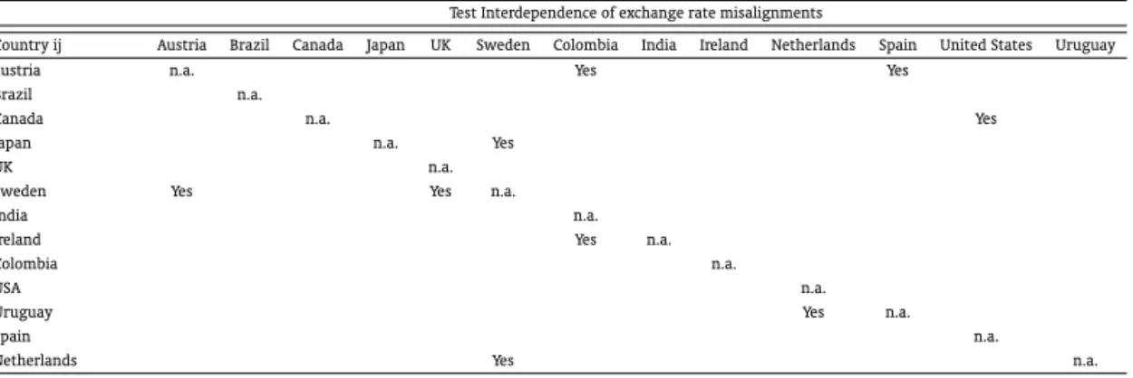
Detailed results for all countries are presented in the appendix (Table 9-Table 19). Table 5 presents the results of the evaluation of the hypothesis that the exchange rate misalignments of a country do not influence the variables in a different country. The country-specific model was expanded to include the misalignment of other countries and then subjected to a simplification algorithm using Oxmetrics. The results suggest that there is little evidence of interdependence via exchange rate misalignment. In other words, misalignments in a country should not generate, as a rule, long-term effects in other countries.

Table 5: Summary of the results of evaluating interdependence using exchange rate misalignment

Test Interdependence of exchange rate misalignments

Country ij Austria Brazil Canada Japan UK Sweden Colombia India Ireland Netherlands Spain United States Uruguay

austria n.a. Yes Yes

Brazil n.a.

Canada n.a. Yes

Japan n.a. Yes

UK n.a.

Sweden Yes Yes n.a.

India n.a.

Ireland Yes n.a.

Colombia n.a.

USA n.a.

Uruguay Yes n.a.

Spain n.a.

Netherlands Yes n.a.

n.a. - not applicable.

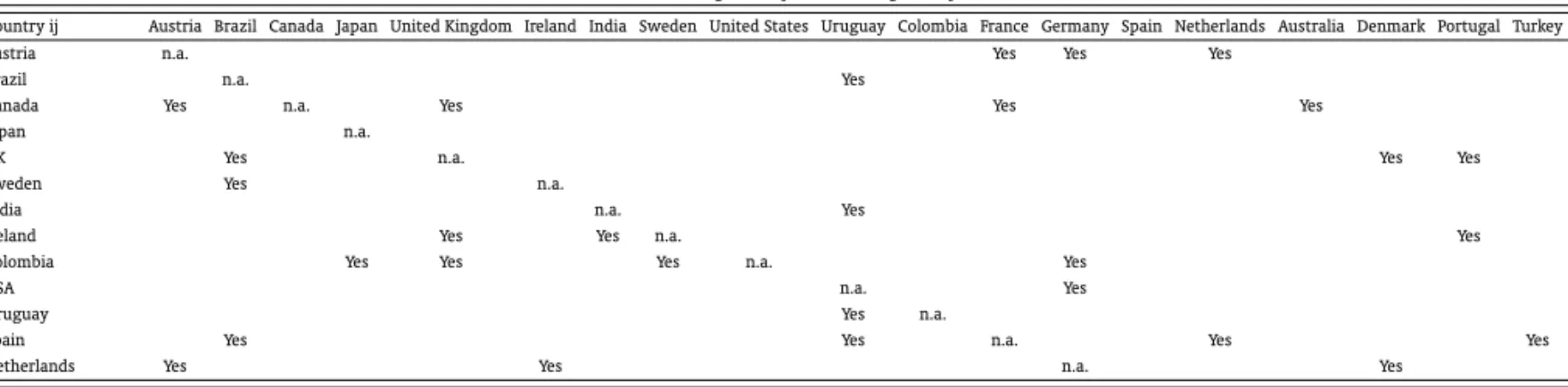
Table 6 presents the results of the strategy that contains the results of a data set that is expanded with not only misalignments but also the first differences of the various variables of other countries. In this case, the evidence for interdependence increases substantially. This finding suggests that in the long run, exchange rates would be simply explained by domestic fundamentals, while in the short run, events in larger economies like the United States or United Kingdom may generate a certain impact on other countries. There is also evidence of a strong regional interconnection among European countries, which was highly expected.

(14)

256

Emerson

Fernandes

Mar

çal

Table 6: Summary of the results of evaluating interdependence among countries using the expanded information data set

Evaluating interdependence using the expanded data set

Country ij Austria Brazil Canada Japan United Kingdom Ireland India Sweden United States Uruguay Colombia France Germany Spain Netherlands Australia Denmark Portugal Turkey

austria n.a. Yes Yes Yes

Brazil n.a. Yes

Canada Yes n.a. Yes Yes Yes

Japan n.a.

UK Yes n.a. Yes Yes

Sweden Yes n.a.

India n.a. Yes

Ireland Yes Yes n.a. Yes

Colombia Yes Yes Yes n.a. Yes

USA n.a. Yes

Uruguay Yes n.a.

Spain Yes Yes n.a. Yes Yes

Netherlands Yes Yes n.a. Yes

n.a. - not applicable.

RBE

Rio

de

Janeiro

v.

68

n.

2

/

p.

243–276

Abr

-Jun

(15)

Finally, the algorithm used permits the identification of the points of instability in the structure. Table 7 presents the points of instability in the expanded models obtained for each country. The findings reinforce the idea that the events in the oil market in the 1970s and the consequent large price increase of oil in international markets had a global impact. Recent events related to the US and European economic crisis also appear to have a global impact.

Table 7: Summary of identified points of instability in the estimated models using exchange rate mis-alignment

Points of Instability in the global model extended by exchange rate misalignment

Country i - Dummy 1973 1974 1975 1976 1977 1979 1980 1981 1983 1984 1985 1986 1993 1994 1999 2000 2001 2002 2003 2005 2006 2008 2009 2010

austria X X X X

Brazil X X X

Canada X

Japan X X X X X X

UK X X X X

Sweden X X X X

India

Ireland X X X X X

Colombia X X X X

USA X X X X X X

Uruguay X X X X X

Spain X X X X X

Netherlands X X X X

X - means significance.

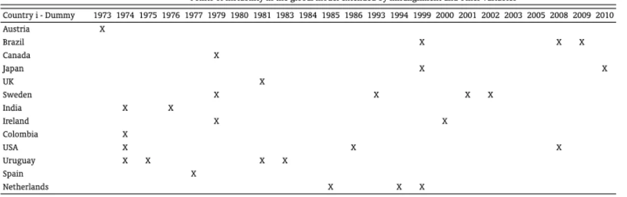
Table 8 presents the results for the expanded data set. The results suggest a smaller number of points of instability, particularly in terms of the events after the 2008 crisis. This suggests that the expanded data set is the most appropriate for explaining the data of several countries. Further, the results may also suggest that the spread of events that followed the 2008 crisis follow a traditional mechanism.

Table 8: Summary of identified points of instability in the estimated models-expanded by misalignment and remaining variables

Points of Instability in the global model extended by misalignment and other variables

Country i - Dummy 1973 1974 1975 1976 1977 1979 1980 1981 1983 1984 1985 1986 1993 1994 1999 2000 2001 2002 2003 2005 2008 2009 2010

Austria X

Brazil X X X

Canada X

Japan X X

UK X

Sweden X X X X

India X X

Ireland X X

Colombia X

USA X X X

Uruguay X X X X

Spain X

Netherlands X X X

(16)

258 6.3. Main findings

The following is a summary of the main conclusions of this study:

a) There is some evidence of interdependence among the analyzed countries in terms of exchange rate. The dynamics of the US data appear to affect a large number of countries. This is in line with the importance of this country in the global economy;

b) There is evidence of strong interdependence among European nations;

c) A shock can only affect the exchange rates of a specific country if it permanently affects its fundamentals;

d) The mechanism of interdependence is restricted mainly to short-term dynamics;

e) Since the error correction mechanisms of a particular country are not important in other coun-tries, there is no reason for not employing Gonzalo and Granger’s decomposition methodology, which is a usual method for estimating exchange rate misalignment.

7. COMPARISON WITH THE RESULTS OF EXISTING LITERATURE

Dufrenot and Mathieu (2006) do not use non-linear models for analyzing exchange rate misalign-ment, but the data set is restricted to data from the countries themselves. Pesaran and Smith (2006) and Pesaran and Smith (2005) attempt to model the phenomena using a global model, although they do not apply the methodology to exchange rate misalignment. The authors seek to identify global factors and assess the extent to which such factors help to improve individual models.

Camarero and Ordónez (2002) estimate exchange rate misalignment using different econometric methodologies:

a) multivariate cointegration of Johansen (1995);

b) panel cointegration techniques Pesaran and Shin (1999).

They obtain similar results in the two methods by analyzing data pertaining to the Euro and dollar. Further, Groen and Kleibergen (2003) conduct a similar analysis to that of Larsson and Lyhagen (2007) and are able to detect interdependence between the dollar and other currencies, as expounded in the monetary approach (Dornbusch (1976) and Mussa (1974) The hypothesis suggested by the monetary approach is not rejected in models in which panel data is used, which is in contrast with models that do not use panel data. In this regard, the results of the abovementioned studies are very close to those of the present study; the only difference lies in the fundamentals used.

Groen and Lombardelli (2004) is also similar to the current study, but their work is limited to model the relationship between the real exchange rate and the Balassa-Samuelson effect without considering the possible effect of the international investment position on the exchange rate.

8. CONCLUSIONS

The objective of this study was to compare different methodologies for determining exchange rate misalignment and test the hypotheses that the exchange rates of different countries are influenced by their own fundamentals as well variables related to the fundamentals of other countries. The second hypothesis is related to the existence of interdependence among countries.

The methodology applied in this study differs from the traditional methodology of calculating ex-change rate misalignment using models containing only variables of the particular country under study

(17)

in that the methodology used in this study permits the expansion of the set of variables to include in-formation related to other countries.

I employed two different empirical strategies for the purpose of such a comparison. The first one was based on evaluating whether a multivariate time series, which is usually used in the literature, containing exchange data pertaining only to the country in question can be improved by adding vari-ables related to other countries. The second strategy was to utilize a long panel data set that includes variables used to estimate exchange rate misalignment and formally test the hypothesis of no interde-pendence.

The results suggested that in both strategies there is some evidence of the existence of interdepen-dence. The source of interdependence appears to be most related to short-term factors. However, it must be noted that the generation of long-term effects of the competitive devaluations in one country on the exchange rate of other countries would imply changing these fundamentals.

BIBLIOGRAPHY

Ahmad, Y. & Craighead, W. D. (2010). Temporal Aggregation and Purchasing Power Parity Persistence.

Journal of International Money and Finance, 30(5):817–830.

Alberola, E. & Cervero, S. (1999). Global Equilibrium exchange rate: Euro, Dolar,“Ins”, “Outs” and other major currencies in a Panel Cointegration Framework. Working Paper 99–175, Washington, IMF.

Beveridge, S. & Nelson, D. B. (1981). A new approach to decomposition of economic time series into permanent and transitory components with particular attention to measuremente of the business cycle. Journal of Monetary Economics, 7(2):151–174.

Bilson, J. F. (1979). Recent developments in monetary models of exchange rate determination. IMF Staff Paper, 26(2):201–223.

Camarero, M. & Ordónez, J. (2002). The euro-dollar exchange rate: is it fundamental? Working paper 798, Venice, CESIFO.

Cavaliere, G. & Rahbek, A. (2008). Testing for Co-Integration in Vector Autoregressions with Non-Stationary Volatility. Journal of Econometrics, 158(10):23.

Clark, P. B. & MacDonald, R. (1998). Exchange rates and economic fundamentals: a methodological comparison of BEERs and FEERs. International Monetary Fund.

Cline, W. R. (2008). Estimating consistent fundamental equilibrium exchange rate. Working paper Series 1–26, Washington, Peterson Institute for International Economics.

Dornbusch, R. (1976). Expectations and Exchange Rate Dynamics. Journal of Political Economy, 84(6):1161–1176.

Dufrenot, G. & Mathieu, L. (2006). Persistent misalignments of the European exchange rates: some evidence from non-linear cointegration. Applied Economics, 38:203–229.

Edwards, S. (1987). Exchange rate misaligment in developing countries. Working paper 442, NBER.

Eichengreen, B. & Sachs, J. D. (1986). Exchange rates and economic recovery in the 1930s. National Bureau of Economic Research Cambridge, Mass, USA.

(18)

260

Faruqee, H. (1995). Long-run determinants of the real exchange rate: A stock Flow Perspective.IMF Staff Paper, 42:80–107.

Froot, K. A. & K. Rogoff, E. (1995). Perspectives on PPP and Long-run Real exchange rates. Handbook of International Economics. Amsterdam, North-Holland.

Glick, R. & Rose, A. K. (1998). Contagion And Trade: Why Are Currency Crises Regional? Working Paper 6806, Washington, NBER.

Gonzalo, J. & Granger, C. W. J. (1995). Estimation of Common Long-Memory Components in Cointegrated Systems. Journal of business and Economics Statistics, 13(1):27–35.

Gredenhoff, M. & Jacobson, T. (2001). Bootstrap Testing Linear Restrictions on Cointegrating Vectors.

Journal of Business & Economic Statistics, 19(1):63–72.

Groen, J. & Lombardelli, C. (2004). Real exchange rates and the relative prices of non-traded and traded goods: an empirical analysis. Working Paper 223, Bank of England.

Groen, J. J. J. & Kleibergen, F. (2003). Likelihood-Based Cointegration Analysis in Panels of Vector Error-Correction Models.Journal of Business & Economic Statistics, 21:295–318.

Hansen, P. R. (2003). Structural changes in the cointegrated vector autoregressive model. Journal of Econometrics, 114:261–295.

Hendry, D. & Krolzig, H. M. (2005). The Properties of Automatic Gets Modelling. Economic Journal, 115:32–61.

Hendry, D. F. (1995). Dynamic Econometrics. Technical report, Oxford, Oxford University Press.

Johansen, S. (1988). Statistical Analysis of cointegration vectors. Journal of Economic Dynamics and Control, 12(2):231–254.

Johansen, S. (1995). Likelihood-based inference in cointegrated vector autoregressive models. Technical report, Oxford, Oxford University Press.

Johansen, S. (1999). A Bartlett correction factor for tests on the cointegrating relations. Technical report, Florence, European University Institute.

Johansen, S. (2000). A small sample correction of the test for cointegrating rank in the vector autore-gressive model. Technical report, Florence, European University Institute.

Juselius, K. (2009). The Cointegrated VAR Model Methodology and Applications Oxford. Technical report, Oxford University Press.

Kubota, M. (2009). Real Exchange Rate Misalignments: Theoretical modelling and empirical evidence. Discussion papers in economics, York, University of York.

Lane, P. R. & Milesi-Ferretti, G. M. (2007). The external wealth of nations mark II: Revised and extended estimates of foreign assets and liabilities, 1970-2004. Journal of International Economics, 73(2):223– 250.

Larsson, R. & Lyhagen, J. (2007). Inference in Panel Cointegration Models with long Panels. Journal of Business and Economic Statistics, 25(4):473–483.

Meese, R. A. & Rogoff, K. (1983). Empirical Exchange models of the seventies: Do they fit out of the sample? Journal of International Economics, 14:3–24.

(19)

Mussa, M. (1974). A Monetary Approach to Balance-of-Payments Analysis. Journal Of Money, Credit And Banking, 6(3):333–351.

Mussa, M. (1976). The exchange rate, the balance of payments and monetary policy under a regime of controlled floating.Scadinavian Journal Of Economics, 78:228–248.

Pesaran, M. H. & Shin, Y. (1999). Pooled Mean Group Estimation of Dynamic Heterogenous Panels.

Journal of American Statistical Association, 94(446):621–634.

Pesaran, M. H. & Smith, L. V. (2005). What if the UK had Joined the Euro in 1999? An Empirical Evaluation using a Global VAR. Technical report, Cambridge, University of Cambridge Faculty of Economics.

Pesaran, M. H. & Smith, R. (2006). Macroeconomic modelling with a global perspective. Technical report, Cambridge, Faculty of Economics University of Cambridge.

Santos, C. & Hendry, D. (2008). Automatic selection of indicators in a fully saturated regression. Compu-tational Statistics, 23(2):317–335.

Shin, Y. (1994). A residual-based test of the null of cointegration against the alternative of no cointegra-tion.Econometric Theory, 10(01):91–115.

Stein, J. (1995). The Fundamental Determinants of the Real Exchange Rate of the U.S. Dollar Relative to Other G-7 Currencies. Working Paper 95–81, IMF.

Swensen, A. R. (2006). Bootstrap algorithms for testing and determining the cointegration rank in VAR models.Econometrica, 74(6):1699–1714.

Taylor, A. M. (2001). Potential Pitfalls for the Purchasing-Power-Parity Puzzle? Sampling and Specifica-tion Biases in Mean-Reversion Tests of the Law of One Price. Econometrica, 69(2):473–498.

Turnovsky, S. J. & Basar, T. (1987). Dynamic Strategic Monetary Policies and Coordination in Interdepen-dent Economies. Working Paper 2467, Washington, NBER.

Ugai, H. (2007). Effects of the quantitative easing policy: A survey of empirical analyses. Monetary And Economic Studies-Bank Of Japan, 25:1–47.

(20)

262 9. APPENDIX A:

In this Appendix, we present the algorithm of the generalized reduced rank regression used to estimate panel VECM parameters and a wild bootstrap procedure to test linear restrictions on panel VECM parameters.

Estimating a panel VECM using generalized reduced rank regression

Defining the following variables and arrays:

Z0t= ∆Xt

Z1t=Xt−1 (5)

Z2t= [∆Xt. . .∆Xt−kDt]

C= (Γ1, . . . ,Γk−1,Φ) (6)

yields

Z0t=AB′Z1t+CZ2t+εt (7)

Hansen (2003) shows how to estimate the process given in (5). Some definitions are now necessary:

vec(B) =Hϕ+h, (8)

where H is known,ϕcontains free parameters,his a tool for normalization, and vec is an operator that transforms a matrix in a column vector.10

vec(A,C) =GΨ (9)

where G is known, andΨcontains free parameters.

Using (6), (7), and (8) to (11), it is possible to estimate the model parameters (see Hansen (2003) for details):

vec(A,b Cb) =G

" G′ T X t=1 " b

B′_Z

1tZ1′tBbBb′Z1tZ2′t

Z2tZ1′tB Zb 2tZ2′t

!

⊗Ω(b t)−1 #

G

#−1

x

xG′

T

X

t=1

vec(Ω(b t)−1

Z0t(Z1′tB,Zb 2′t)) (10)

vec(Bb) =H

"

H′

T

X

t=1

(Ab′Ω(b t)−1_b

A⊗Z1tZ1′t)H

#−1

x xH′ " H′ T X t=1

vec(Z1t(Z0t−CZb 2t)′Ω(b t)−1Ab)− T

X

t=1

vec(Ab′Ω(b t)−1_b

A⊗Z1tZ1′t)h

#

+h (11)

10_{Further details regarding the properties of such an operator can be found in a more advanced book of econometrics. For}

example Hendry (1995). Dynamic Econometrics. Oxford, Oxford University Press., or Lutkepohl, H. (2007). New introduction to multiple time series analysis, Springer.

(21)

Ω = (T)−1

T

X

t=1 b

εtεb′t, (12)

b

εt=Zot−AbBb′Z1t+CZb 2t. (13)

After convergence is attained according to some established criterion, the likelihood function can be calculated. Based on the values of the restricted and unrestricted general model, it is possible to calculate a likelihood ratio test with an asymptotic chi-squared distribution Larsson and Lyhagen (2007).

Testing linear restrictions on panel VECM parameters

The likelihood ratio procedure described in the previous section suffers from a serious distortion. This encourages analysts to use a bootstrap technique to obtain appropriate critical values. Studies that discuss similar problems are Johansen (1999), Johansen et alii (2000), Gredenhoff and Jacobson (2001), and Swensen (2006). We chose to perform a bootstrap to simulate the appropriate distribution for the test statistic. The results suggest that the size distortion is actually severe.

The procedure used is a wild bootstrap similar to that used in Cavaliere and Rahbek (2008):11

Step 1: Estimate the model given by equation (3) under the null and alternative hypothesis and calcu-late the statistic likelihood ratio.

Step 2: Save the model parameters estimated under the null hypothesis and check the stability of the system. If the system is stable, proceed to Step 3. If not, abort the procedure.

Step 3: Construct the errors for generating artificial data using equation (12) below from the parame-ters estimated with the model constraints on the null hypothesis:

b

ut≡bεtwt, (14)

whereεbtis defined as in (11) andwt∼N I(0,1).,

Step 4: Generate the Q series with the sample size T from equation (1) with the parameter structure of the null hypothesis.

Step 5: Perform the likelihood ratio test described in Step 1 for all artificially generated samples. The values of the test statistics are retained. Calculate the p-value by dividing the total number of times the value of the likelihood ratio statistic obtained with the real sample data is greater than value of the likelihood ratio statistic obtained with artificial data divided by the number of runs.

(22)

264 10. APPENDIX B: COMPLEMENTARY TABLES

Table 9: Final model selected using the Ox algorithm: Canada.

Canada

Model 1

CIa_spa_1 I:1973 I:1979 I:1986 I:2008 Constant CIa_canada_1 DLRER_t Coefficient -0,0405 -0,0635 0,3249 -0,1633 -0,0680 -6,6033 0,0386

Standard Error 0,0112 0,0503 0,0492 0,0504 0,0489 1,6940 0,0105 t -3,6200 -1,2600 6,6000 -3,2400 -1,3900 -3,9000 3,6700

p-value 0,10% 21,61% 0,00% 0,28% 17,37% 0,05% 0,09%

DLNFA_t Coefficient 0,011 0,053 -0,035 0,001 0,069 1,259 0,000 Standard Error 0,008 0,036 0,036 0,036 0,035 1,224 0,008

t 1,390 1,470 -0,993 0,036 1,960 1,030 -0,025

p-value 17,44% 15,13% 32,82% 97,15% 5,86% 31,12% 98,02% DLBS_t Coefficient 0,021 -0,041 0,003 0,050 -0,012 3,522 -0,021

Standard Error 0,006 0,025 0,025 0,025 0,024 0,843 0,005

t 3,830 -1,630 0,111 2,010 -0,482 4,180 -4,020

p-value 0,06% 11,31% 91,25% 5,29% 63,27% 0,02% 0,03% Model 2

CIa_spa_1 DLRER_aus_1 DLRER_aut_1 DLRER_uni_1 I:1979 Constant CIa_canada_1 DLRER_t Coefficient -0,0258 0,1455 0,2499 -0,0034 0,3392 -4,5778 0,0312

Standard Error 0,0105 0,3660 0,3413 0,1256 0,0514 1,6300 0,0106 t -2,4500 0,3980 0,7320 -0,0269 6,6000 -2,8100 2,9300 p-value 1,99% 69,36% 46,93% 97,87% 0,00% 0,84% 0,61% DLNFA_t Coefficient 0,005 -0,156 0,238 -0,240 -0,025 0,309 0,004 Standard Error 0,007 0,234 0,218 0,080 0,033 1,043 0,007

t 0,685 -0,668 1,090 -2,990 -0,766 0,297 0,569

p-value 49,85% 50,90% 28,49% 0,54% 44,91% 76,87% 57,35% DLBS_t Coefficient 0,022 -0,231 0,053 0,074 0,002 3,582 -0,021

Standard Error 0,005 0,170 0,158 0,058 0,024 0,756 0,005

t 4,470 -1,360 0,335 1,270 0,074 4,740 -4,280

p-value 0,01% 18,28% 74,00% 21,37% 94,15% 0,00% 0,02%

Note: Cla denotes the cointegration vector

(23)

Table 10: Final model selected using the Ox algorithm: Austria.

Austria Model 1

CIa_india_1 CIa_uru_1 I:1973 I:1985 I:1986 I:2009 Constant CIa_austria_1 DLRER_t Coefficient -0,0268 -0,0081 0,0712 -0,2013 -0,1515 -0,0859 1,8263 0,0175

Standard Error 0,0088 0,0115 0,0517 0,0582 0,0601 0,0535 0,8268 0,0099 t -3,0600 -0,7050 1,3800 -3,4600 -2,5200 -1,6100 2,2100 1,7700 p-value 0,46% 48,59% 17,84% 0,16% 1,71% 11,85% 3,47% 8,65% DLNFA_t Coefficient 0,007 -0,002 0,005 -0,033 -0,002 0,087 -1,647 -0,020 Standard Error 0,006 0,008 0,035 0,039 0,041 0,036 0,558 0,007 t 1,130 -0,281 0,157 -0,843 -0,057 2,400 -2,950 -3,050 p-value 26,67% 78,04% 87,64% 40,54% 95,46% 2,25% 0,60% 0,47% DLBS_t Coefficient -0,003 0,006 -0,071 0,016 -0,015 -0,047 0,537 0,006 Standard Error 0,002 0,002 0,011 0,012 0,012 0,011 0,168 0,002 t -1,970 2,350 -6,740 1,350 -1,190 -4,330 3,190 3,070 p-value 5,83% 2,52% 0,00% 18,54% 24,18% 0,01% 0,32% 0,44%

Model 2

DLpreco_relativo_ger_1 DLRER_net_1 Dnfa_spa_1 I:1973 Constant U CIa_austria_1 DLRER_t Coefficient -0,7996 0,8636 -0,4571 0,0417 -0,3130 -0,0042

Standard Error 0,6591 0,2869 0,1603 0,0584 0,7003 0,0095 t -1,2100 3,0100 -2,8500 0,7140 -0,4470 -0,4370 p-value 23,37% 0,50% 0,75% 48,02% 65,79% 66,46% DLNFA_t Coefficient 0,3231 0,2349 -0,0607 0,0124 -1,1899 -0,0160 Standard Error 0,4181 0,1820 0,1017 0,0370 0,4442 0,0060 t 0,7730 1,2900 -0,5970 0,3350 -2,6800 -2,6600 p-value 44,52% 20,57% 55,45% 74,00% 1,14% 1,19% DLBS_t Coefficient 0,273 0,060 -0,121 -0,059 0,240 0,003 Standard Error 0,139 0,061 0,034 0,012 0,148 0,002

t 1,960 0,987 -3,570 -4,820 1,620 1,680

p-value 5,82% 33,06% 0,11% 0,00% 11,38% 10,27%

(24)

266

Table 11: Final model selected using the Ox algorithm: Colombia.

Colombia Model 1

Dnfa_col_1 CIa_uni_1 I:1974 I:1977 I:1986 I:2001 Constante CIa_col_1 DLRER_t Coefficient -0,613 0,013 0,089 0,191 -0,189 -0,009 1,321 -0,042

Standard Error 0,249 0,009 0,058 0,059 0,062 0,061 0,246 0,008

t -2,460 1,430 1,540 3,250 -3,070 -0,152 5,370 -5,400

p-value 0,020 0,163 0,135 0,003 0,004 0,880 0,000 0,000

DLNFA_t Coefficient 0,778 0,011 -0,013 -0,035 0,026 -0,109 -0,423 0,013 Standard Error 0,176 0,007 0,041 0,042 0,044 0,043 0,174 0,005

t 4,410 1,640 -0,313 -0,841 0,606 -2,510 -2,430 2,450

p-value 0,000 0,111 0,756 0,407 0,549 0,018 0,021 0,020

DLBS_t Coefficient 0,024 -0,011 0,069 -0,036 0,018 0,039 -0,379 0,012 Standard Error 0,103 0,004 0,024 0,024 0,026 0,025 0,102 0,003

t 0,228 -2,880 2,860 -1,480 0,722 1,520 -3,710 3,710

p-value 82,08% 0,72% 0,75% 14,77% 47,56% 13,86% 0,08% 0,08% Model 2

Dnfa_col_1 DLpreco_relativo_jap_1 Dnfa_ire_1 Dnfa_net_1 Dnfa_spa_1 I:1974 Constante CIa_col_1 DLRER_t Coefficient -0,2543 -0,2278 0,0522 0,1370 -0,3956 0,0687 1,4490 -0,0461

Standard Error 0,2792 0,2027 0,0682 0,1195 0,2023 0,0702 0,2853 0,0089 t -0,9110 -1,1200 0,7650 1,1500 -1,9600 0,9780 5,0800 -5,1800 p-value 36,95% 26,96% 44,99% 26,04% 5,96% 33,56% 0,00% 0,00% DLNFA_t Coefficient 0,595 -0,276 0,133 0,164 -0,131 -0,025 -0,250 0,008 Standard Error 0,126 0,092 0,031 0,054 0,092 0,032 0,129 0,004

t 4,710 -3,010 4,290 3,030 -1,440 -0,782 -1,940 1,900

p-value 0,00% 0,52% 0,02% 0,49% 16,11% 44,02% 6,21% 6,70% DLBS_t Coefficient -0,089 -0,066 -0,057 -0,061 0,266 0,066 -0,420 0,013 Standard Error 0,084 0,061 0,021 0,036 0,061 0,021 0,086 0,003

t -1,060 -1,080 -2,740 -1,690 4,360 3,110 -4,880 4,940

p-value 29,88% 28,79% 1,00% 10,09% 0,01% 0,40% 0,00% 0,00%

(25)

Table 12: Final model selected using the Ox algorithm: United Kingdom.

United Kindgom

I:1973 I:1981 I:1984 I:2009 Constant CIa_uni_1 DLRER_t Coefficient -0,105 0,011 0,197 -0,012 0,006 0,005

Standard Error 0,058 0,058 0,059 0,058 0,010 0,009

t -1,810 0,187 3,310 -0,205 0,640 0,597

p-value 7,96% 85,29% 0,22% 83,85% 52,69% 55,44% DLNFA_t Coefficient -0,008 0,061 0,067 -0,177 -0,004 0,020

Standard Error 0,060 0,060 0,061 0,059 0,010 0,009

t -0,142 1,030 1,100 -2,980 -0,415 2,120

p-value 88,82% 31,04% 28,10% 0,54% 68,11% 4,16% DLBS_t Coefficient -0,078 0,147 0,013 0,070 0,002 -0,008 Standard Error 0,030 0,030 0,030 0,030 0,005 0,005

t -2,610 4,950 0,412 2,370 0,419 -1,680

p-value 1,36% 0,00% 68,27% 2,40% 67,81% 10,16% Model 2

DLRER_por_1 Dnfa_bra_1 Dnfa_den_1 I:1981 Constant CIa_uni_1 DLRER_t Coefficient -0,5112 -0,2089 -0,1362 0,0032 0,0097 0,0025

Standard Error 0,2184 0,1514 0,2044 0,0624 0,0100 0,0099 t -2,3400 -1,3800 -0,6660 0,0506 0,9750 0,2540 p-value 2,54% 17,68% 50,97% 95,99% 33,67% 80,14% DLNFA_t Coefficient 0,093 -0,645 -0,548 0,025 -0,007 0,015

Standard Error 0,154 0,106 0,144 0,044 0,007 0,007

t 0,608 -6,060 -3,810 0,573 -1,000 2,130

p-value 54,77% 0,00% 0,06% 57,05% 32,38% 4,08% DLBS_t Coefficient 0,361 0,044 -0,158 0,143 0,002 -0,006 Standard Error 0,101 0,070 0,095 0,029 0,005 0,005

t 3,570 0,626 -1,670 4,940 0,485 -1,230

p-value 0,11% 53,54% 10,45% 0,00% 63,07% 22,66%

(26)

268

Table 13: Final model selected using the Ox algorithm: India

India Model 1

Dnfa_ind_1 I:1974 I:1976 I:1993 I:2009 Constant U CIa_india_1 U DLRER_t Coefficient 0,726 0,135 -0,117 0,124 -0,074 0,539 -0,0284

Standard Error 0,435 0,057 0,056 0,061 0,059 0,174 0,0087

t 1,670 2,380 -2,080 2,030 -1,250 3,100 -3,2700

p-value 10,49% 2,35% 4,60% 5,11% 22,18% 0,40% 0,26% DLNFA_t Coefficient 0,720 -0,006 0,027 0,063 -0,009 -0,011 0,000 Standard Error 0,132 0,017 0,017 0,019 0,018 0,053 0,003

t 5,460 -0,367 1,580 3,380 -0,473 -0,216 0,186

p-value 0,00% 71,58% 12,47% 0,19% 63,97% 83,07% 85,34% DLBS_t Coefficient -0,041 -0,074 -0,020 -0,021 0,056 -0,162 0,008

Standard Error 0,109 0,014 0,014 0,015 0,015 0,043 0,002

t -0,374 -5,240 -1,410 -1,360 3,790 -3,720 3,880

p-value 71,08% 0,00% 16,88% 18,31% 0,06% 0,08% 0,05% Model 2

Dnfa_ind_1 DLpreco_relativo_usa Dnfa_usa_1 I:1974 I:1976 Constant CIa_india_1 DLRER_t Coefficient 0,6724 -0,2451 0,4215 0,1345 -0,1429 0,3377 -0,0181

Standard Error 0,4217 0,1161 0,2970 0,0560 0,0559 0,1555 0,0078 t 1,5900 -2,1100 1,4200 2,4000 -2,5600 2,1700 -2,3300 p-value 12,06% 4,27% 16,56% 2,23% 1,55% 3,74% 2,61% DLNFA_t Coefficient 0,673 -0,049 -0,031 -0,010 0,022 -0,070 0,004 Standard Error 0,149 0,041 0,105 0,020 0,020 0,055 0,003

t 4,530 -1,210 -0,297 -0,492 1,120 -1,290 1,290

p-value 0,01% 23,63% 76,86% 62,59% 26,91% 20,78% 20,78% DLBS_t Coefficient -0,040 0,071 -0,355 -0,078 -0,008 -0,074 0,004

Standard Error 0,082 0,022 0,057 0,011 0,011 0,030 0,002

t -0,486 3,160 -6,180 -7,250 -0,710 -2,460 2,640

p-value 63,03% 0,34% 0,00% 0,00% 48,27% 1,96% 1,27%

(27)

Table 14: Final model selected using the Ox algorithm: Ireland.

Ireland Model 1

CIa_india_1 I:1974 I:1979 I:2000 I:2003 I:2009 Constant CIa_ire_1 DLRER_t Coefficient -0,011 -0,006 0,170 -0,053 0,084 -0,067 -0,0160 -0,00377426

Standard Error 0,006 0,038 0,038 0,038 0,038 0,041 0,4208 0,007132 t -1,860 -0,145 4,450 -1,400 2,200 -1,640 -0,0381 -0,529 p-value 7,31% 88,55% 0,01% 17,17% 3,57% 11,17% 96,99% 0,6004 DLNFA_t Coefficient 0,013 -0,022 -0,019 -0,584 -0,007 -0,197 -3,921 -0,056 Standard Error 0,021 0,131 0,131 0,130 0,130 0,139 1,436 0,024 t 0,613 -0,169 -0,143 -4,500 -0,050 -1,420 -2,730 -2,290 p-value 54,44% 86,70% 88,74% 0,01% 96,02% 16,57% 1,03% 2,92% DLBS_t Coefficient 0,019 0,027 0,261 -0,019 -0,004 0,015 0,761 0,017 Standard Error 0,006 0,137 0,082 0,105 0,035 0,044 0,364 0,006 t 3,370 0,199 3,170 -0,180 -0,110 0,337 2,090 2,790 p-value 0,20% 84,39% 0,34% 85,85% 91,34% 73,87% 4,49% 0,90%

Model 2

CIa_india_1 Dnfa_den_1 Dnfa_gre_1 Dnfa_uni_1 I:1979 I:2000 Constant CIa_ire_1 DLRER_t Coefficient -0,010 -0,355 -0,154 0,117 0,168 -0,020 -0,3820 -0,00872603

Standard Error 0,006 0,136 0,081 0,104 0,034 0,043 0,3596 0,006191 t -1,690 -2,620 -1,890 1,130 4,880 -0,456 -1,0600 -1,41 p-value 10,09% 1,36% 6,78% 26,66% 0,00% 65,15% 29,63% 0,1686 DLNFA_t Coefficient 0,022 0,471 -0,042 -0,861 0,034 -0,566 -4,107 -0,056 Standard Error 0,019 0,450 0,269 0,344 0,114 0,143 1,193 0,021 t 1,160 1,050 -0,157 -2,500 0,297 -3,950 -3,440 -2,710 p-value 25,69% 30,28% 87,66% 1,80% 76,82% 0,04% 0,17% 1,10% DLBS_t Coefficient 0,028 -0,109 0,007 0,007 -0,085 0,131 0,440 0,015 Standard Error 0,004 0,023 0,023 0,023 0,023 0,025 0,256 0,004 t 7,390 -4,650 0,290 0,318 -3,650 5,290 1,720 3,520 p-value 0,00% 0,01% 77,41% 75,26% 0,10% 0,00% 9,61% 0,14%

(28)

270

Table 15: Final model selected using the Ox algorithm: Japan.

Japan Model 1

CIa_swe_1 I:1975 I:1999 I:2005 I:2010 Constant CIa_jap_1 DLRER_t Coefficient 0,0366 -0,0370 0,1298 -0,0916 -0,0024 2,7562 -0,0093

Standard Error 0,0151 0,0938 0,0933 0,0946 0,1027 1,1780 0,0153 t 2,4200 -0,3940 1,3900 -0,9690 -0,0237 2,3400 -0,6050 p-value 2,14% 69,63% 17,38% 33,98% 98,13% 2,57% 54,92% DLNFA_t Coefficient -0,014 0,045 -0,153 -0,088 -0,083 -0,806 -0,012 Standard Error 0,004 0,024 0,024 0,024 0,027 0,305 0,004 t -3,630 1,860 -6,350 -3,620 -3,120 -2,650 -3,020 p-value 0,10% 7,28% 0,00% 0,10% 0,38% 1,25% 0,49% DLBS_t Coefficient -0,021 -0,119 -0,087 0,056 0,253 -1,707 0,013 Standard Error 0,008 0,052 0,051 0,052 0,057 0,649 0,008 t -2,510 -2,310 -1,700 1,080 4,470 -2,630 1,520 p-value 1,74% 2,77% 9,95% 28,72% 0,01% 1,30% 13,78%

Model 2

DLpreco_relativo_1 I:1999 I:2010 Constant CIa_jap_1 DLRER_t Coefficient -0,1842 0,0926 0,0111 -0,0954 0,0073

Standard Error 0,2031 0,0966 0,1069 0,2191 0,0143 t -0,9070 0,9580 0,1030 -0,4350 0,5070 p-value 37,07% 34,48% 91,82% 66,60% 61,57% DLNFA_t Coefficient 0,033 -0,133 -0,068 0,207 -0,012 Standard Error 0,068 0,032 0,036 0,073 0,005 t 0,480 -4,130 -1,920 2,830 -2,610 p-value 63,40% 0,02% 6,34% 0,77% 1,32% DLBS_t Coefficient -0,158 -0,067 0,227 -0,043 0,001 Standard Error 0,118 0,056 0,062 0,128 0,008 t -1,330 -1,190 3,640 -0,333 0,103 p-value 19,19% 24,20% 0,09% 74,13% 91,82%