Assessing Interdependence Among Countries’
Fundamentals and its Implications for Exchange
Rate Misalignment Estimates: An Empirical
Exercise Based on GVAR
*
Emerson Fernandes Marçal†, Beatrice Zimmermann‡, Diogo de Prince§, Giovanni Merlin¶
Contents
1. Introduction ...429 2. A short review of exchange
rate misalignment
literature ...430 3. Methodologies to calculate
exchange rate
misalignment...432 4. Results ...436 5. Final remarks ...446
Keywords
Real effective exchange rate, cointegration, global VAR
JEL Codes
C52, F31, F37
Abstract·Resumo
Exchange rates are important macroeconomic prices and changes in these rates affect economic activity, prices, interest rates, and trade flows. Methodologies have been developed in empirical exchange rate misalignment studies to evaluate whether a real effective exchange is overvalued or undervalued. There is a vast body of literature on the determinants of long-term real exchange rates and on empirical strategies to implement the equilibrium norms obtained from theoretical models. This study seeks to contribute to this literature by showing that the global vector autoregressions model (GVAR) proposed byPesaran, Schuermann, and Weiner(2004) can add relevant information to the literature on measuring exchange rate misalignment. Our empirical exercise suggests that the estimate exchange rate misalignment obtained from GVAR can be quite different to that using the traditional cointegrated time series techniques, which treat countries as detached entities. The differences between the two approaches are more pronounced for small and developing countries. Our results also suggest a strong interdependence among eurozone countries, as expected.
1. Introduction
The exchange rate is an important macroeconomic price and changes in these rates affect economic activity, prices, interest rates, and trade flows. Large changes in an exchange rate always generate debate on whether the movements are “excessive”, reflect “fundamentals”, or are “rational”. Empirical studies have developed models to assess the long-term determinants of real exchange rates. Empirical strategies are then formulated based on these models, using the doctrine of purchasing power parity (PPP), or based on a fundamentals analysis.
*The authors acknowledge the comments from the participants of the first International Annual Applied Econometric Conference, fourth Emerging Market Group Conference, fourteenth OxMetrics User Conference. The authors also acknowledge Joseph Gagnon, Luis Catão, Irineu Evangelista, Pedro Valls, Megumi Kubota, Cesar Calderon, Aluisio de Lima Campos and Vera Thorstensen for helpful comments on a very preliminary version of this work. All remaining errors are the responsibility of the authors.
†Fundação Getulio Vargas, Escola de Economia de São Paulo, Centro de Macroeconomia Aplicada (FGV/EESP/CEMAP). Rua Itapeva 286, 10º andar, São Paulo, SP, CEP 01332-000, Brasil. This author acknowledges partial financial support received from CNPQ (Grant number 311044/2013-1) and from WTO Chair Project.
‡World Bank, DIME. Setor Comercial Norte, Quadra 2, Lote A, Edifício Corporate Financial Center, 7° andar, Brasília, DF, CEP 70712-900, Brasil.
§Universidade Federal de São Paulo, Escola Paulista de Política, Economia e Negócios (Unifesp/EPPEN). Address: Rua Angélica,100, Jd. das flores, Osasco, SP, 06110-295, Brazil.
¶PhD in Economics at Escola de Economia de São Paulo. Dorfstrasse 9, 8800, Thalwil, Switzerland.
[email protected] [email protected] [email protected] [email protected]
This is an open-access article distributed under the terms of the Creative Commons Attribution License.
Many studies have attempted to construct more accurate estimates of the magnitude and sign of exchange rate misalignment. Exchange rate misalignment is defined as the difference between a measure of the real exchange rate and some equilibrium norm. Discussions on exchange rate misalignment can be divided into two levels. The first focuses on which is the best norm to use to evaluate exchange rate equilibrium. Economic models give a better understanding of the determinants of the real exchange rate. These models attempt to determine the best set of fundamentals that explain real effective exchange rates in the long run. The second level of debate revolves around the best empirical strategy to measure exchange rate equilibrium norms. This is an econometric debate.
Empirical studies also need to choose between a time series or panel approach. The time series approach has the advantage of allowing a particular structure to be estimated for each country. However, the approach does not allow a broader set of variables to be analyzed at the same time because the available macroeconomic samples are not long enough. Panel techniques allow analysts to enlarge the spectrum of variables, but at the cost of imposing untested similarities between the parameters of different countries’ models. Hossfeld(2010) reviews exchange rate misalignment literature, and evaluates the benefits and limits of the time series and panel approaches.
This study seeks to contribute to the current body of literature by showing that the global vector autoregressions model (GVAR) proposed byPesaran, Schuermann, and Weiner(2004) can be used to model the interdependence between countries. In addition, the model can add relevant information to the literature on measuring exchange rate misalignment. As far as the authors are aware, this approach has not been applied to exchange rate misalignment estimation.
This paper is divided into five sections. The first is this introduction.Section 2provides a brief review of current literature on exchange rate misalignment determinants and describes the challenges faced by empirical studies in trying to determine whether a country’s exchange rate is overvalued or undervalued.Section 3presents the global vector autoregressive model and explains how to adapt Gonzalo and Granger’s methodology to this framework.Section 4 describes the results of an empirical exercise that models real effective exchange rates for a selected group of countries. Here, we also present a comparative analysis of the traditional time series approach and the GVAR approach to exchange rate misalignment. Our results suggest that the GVAR approach is worth considering.section 5applies the limits and the merits of the GVAR approach to the exchange rate misalignment problem and suggests possible extensions to our work. This section also concludes the paper.
2. A short review of exchange rate misalignment literature
The literature on real exchange rates is extensive (Froot & Rogoff,1995). The classical doctrine, and perhaps the oldest one on real exchange rate determinants is that of purchasing power parity (PPP). Reference to this theory can be found in classic studies. Recent studies confirm the validity of PPP for tradable goods, although the adjustment towards equilibrium is quite slow.Ahmad and Craighead(2011) obtained strong evidence of a mean reversion with a high half-life using a secular consumer price index dataset for the United States and United Kingdom. Their work investigates the point made byTaylor(2001) on the effects of temporal aggregation on PPP tests.
the causes and consequences of exchange rate misalignment, andDornbusch(1976), who developed the classic flexible exchange rate model approach under which monetary policy shocks cause deviations from PPP fundamentals.
The studies ofBilson(1979) andMussa(1976) are also classics. These are key references for the monetary approach to exchange rates. Under this approach, the exchange rate would be primarily driven by two fundamentals: the difference between domestic and foreign income, and the money supply. The approach assumes that PPP and uncovered interest parity (UIP) hold continuously, and that the demand for money is stable in all countries. However, the research byMeese and Rogoff(1983) casts doubt on the explanatory power of this theory by showing that the predictions of this approach are not superior to a “naive” forecast model for exchange rates, such as a pure random walk.Rossi(2013) shows that the random walk can be outperformed by an econometric model that uses information based on net foreign investment position. “Predictability is most apparent when one or more of the following hold: the predictors are Taylor rule and net foreign assets fundamentals; the model is linear; and a small number of parameters are estimated”Rossi(2013).
Stein(1995) formulated the natural exchange rate approach (NATREX). According to the author, the equilibrium exchange rate is one that is equal to the level of investment and savings generated by economic fundamentals.
Williamson(1994) had a significant impact on exchange rate misalignment theory. Here, the equilibrium exchange rate is the one that allows a country to sustain a desirable result in its external accounts. This is referred to as the fundamental real exchange rate approach (FRER). A more recent reference to this approach is that ofCline and Williamson(2008). A limitation of this approach is that choosing the target of foreign accounts is highly arbitrary and subjective. As a result, the results may not be robust to different targets. In addition, this approach focuses on flows, not stocks.
Faruqee(1995) incorporates the evolution of stocks and constructed a model that allows flows and stocks to interact. Thus, there must be a stable relationship between the real exchange rate and the net foreign asset position between residents and non-residents. This is referred to as the behavioral real exchange rate (BRER) approach. The model was subsequently extended byAlberola, Cervero, Lopez, and Ubide(1999).
Kubota(2009) includes a representative agent who maximizes intertemporal consump-tion and accumulates capital. This study indicates that the real exchange rate is a funcconsump-tion of terms of trade, net external position, and the relative productivity of the tradable and non-tradable sectors. This approach seeks to reduce the degree of subjectivity when estimating exchange rate misalignment. To this end, she establishes a link between the real exchange rate and a set of fundamentals derived from a theoretical model. She then decomposes the series of real exchange rates into transitory and permanent components using the time series econometric technique.
Recently, the International Monetary Fund (IMF) began to systematically disseminate its research efforts into measuring the exchange rate misalignment in several of its member countries (IMF,2013). Two documents were recently released. These works are an important advance towards transparency. The codes and dataset used to calculate the exchange rate misalignment are available on the IMF website, and the results are easy to replicate. The methodology is also a step forward in incorporating the role of policy gaps in exchange rate misalignment estimates.
real effective exchange rate (REER) indices.1 The basic idea is that the REER can be written
as a function of the output gap, real interest rate differential, and factors that may affect saving, investment, current account, capital flows, and changes in foreign currency reserves.
The explanatory variables included in the EBA model are the commodity terms of trade, trade openness, share of administered prices, VIX,2 the share of own currency in
world reserves, financial home bias, population growth, expected GDP growth over the next five years, productivity, and changes in foreign reserves. The following policy-related regressors are also included: health expenditure to GDP, foreign exchange interventions, real short-term interest rate differential, private credit to GDP, and capital controls. Most of the variables described are relative to the country’s trade partners. They use the same weights as the REER calculation and/or interact with capital account openness. In addition, some variables are lagged to control for endogeneity. The sample data covers 40 countries over the period 1990–2010. The model includes countries fixed effects. To guarantee multilateral consistency in the results, the exchange rate misalignment must be adjusted.
Given the results of the estimation, the “Total REER Gap” can be calculated as the sum of the regression residual and the “Total Policy Gap”. The policy gap is a measure of a cyclical gap (over a benchmark) in six policy areas: fiscal balance, capital controls, social spending, foreign exchange market intervention, financial policies, and monetary policy. The gap is calculated as the difference between the actual level of the variable and its “desirable” level, multiplied by the value of the estimated coefficient. The “desirable” levels are supplied by the desk of each IMF country.
3. Methodologies to calculate exchange rate misalignment
3.1 Traditional time series approach
The analysis starts with an estimation of a vector error correction model (VECM), as suggested byJohansen(1988,1995). The model is given by equation (1):
Δ𝑥𝑖𝑡= 𝛼𝑖𝛽𝑖′𝑥𝑖,𝑡−1+ Γ𝑖1Δ𝑥𝑖,𝑡−1+ ⋯ + Γ𝑖,𝑘−1Δ𝑥𝑖,𝑡−𝑘+1+ Φ𝑖𝐷𝑡+ 𝜀𝑖𝑡, (1)
where𝜀𝑖𝑡are not correlated random errors. The vector𝑥𝑖𝑡contains the variables for the real
exchange rate and the fundamentals (e.g., net foreign investment position, etc.) and has dimension𝑝;𝐷𝑡contains deterministic terms; and𝜃 = {𝛼𝑖, 𝛽𝑖, Γ𝑖1, … , Γ𝑖,𝑘−1, Φ𝑖}is the set
of parameters to be estimated.
The Gonzalo and Granger decomposition
Several decompositions have been proposed to decompose the series into transitory and permanent components. The decomposition ofGonzalo and Granger(1995) is widely used in exchange rate misalignment empirical literature.3 In their decomposition, the transitory
components do not cause changes in the permanent component in the long term. In other words, exchange rate misalignment — defined as the transitory component of the real exchange rate in a multivariate equation system — does not contain relevant information for predicting the changes of the permanent components in the long term.
1A full description of the methodology, data, and routines are available athttp://www.imf.org/external/np/spr/
2013/esr/
2Chicago Board Options Exchange Market Volatility Index.
Using the parameters from (1), it is possible to calculate the transitory component (𝑇𝑖𝑡)
and the permanent component (𝑃𝑖𝑡) from the following equations:
𝑃𝑖𝑡= 𝛽𝑖(𝛼𝑖⟂′ 𝛽𝑖⟂)−1𝛼𝑖⟂′ 𝑥𝑖𝑡, (2)
𝑇𝑖𝑡= 𝛼𝑖(𝛽′
𝑖𝛼𝑖)−1𝛽𝑖′𝑥𝑖𝑡. (3)
The estimate of exchange rate misalignment is the component associated with the position of the real exchange rate in vector𝑥𝑖𝑡. Assuming that the real exchange rate is in the first position of the vector, and using the value of the error correction mechanism centered on their own means, one can calculate the misalignment using the following equation:
mis𝑖𝑡≡ [1 0 ⋯ 0] 𝛼𝑖(𝛽𝑖′𝛼𝑖)−1(𝛽′
𝑖𝑥𝑖𝑡−𝔼[𝛽𝑖′𝑥𝑖𝑡]). (4)
3.2 Motivation for a global model
The severity of the U.S. economic crisis in 2008 brought the fear of a strong negative contagion to the rest of the world. The U.S. authorities have subsequently adopted an aggressive monetary policy with a strong reduction in nominal interest rates and monetary expansion, among other measures. Some analysts may argue that this policy could have generated strong pressure to depreciate the U.S. dollar against currencies whose domestic interest rates did not follow the same movement. Countries that did not follow such a reduction and opted to accumulate reserves to prevent the appreciation of their currency could have faced inflationary pressures. Some authors argue that the United States was using its monetary policy to depreciate its currency, thereby fostering aggregate demand to reduce the intensity and duration of the economic slowdown. This policy may have generated repercussions around the world. There is much discussion about the extension of these effects and whether they are deleterious.
We construct a global model to assess the magnitude of effects, similar to those discussed in the previous paragraph. In this context, the GVAR appears to be an interesting option, as the relevance and magnitude of global factors, vis-a-vis domestic components, can be explicitly and properly evaluated and tested.
3.2.1 GVAR model
In this study, we apply the GVAR methodology to ascertain whether there is any external factor affecting the real exchange rate in the long or short run for a group of selected countries. In this sense, the measure of exchange rate misalignment may have two components. The first is related to domestic fundamentals and the second to global factors. The GVAR explains the source of external influences on the domestic economy by including external variables in VARX.4External variables are usually assumed to be weakly exogenous for each country,
as defined inEngle, Hendry, and Richard(1983) andHendry(1995).
In general, the GVAR can be described as a two-step approach. In the first step, a specific model for each country is estimated using the variables of the country and the trading partners weighted average of external variables. Then, all individual models are stacked and grouped into a system of equations, which are solved. Once this is done, the model provides options for different types of analyses, such as the forecast evaluation and impulse response
analysis. Overall, there is a set of individual models represented as VARX that are combined to obtain the GVAR.
Following the notation ofPesaran et al.(2004), we restrict our discussion to the spec-ification with first-order dynamics, as represented by VAR(1, 1). We consider a set of𝑁
countries and the VAR(1, 1)below:
𝑥𝑖𝑡= 𝑎𝑖,0+ 𝑎𝑖,1𝑡 + Φ𝑖𝑥𝑖,𝑡−1+ Λ𝑖,0𝑥∗𝑖,𝑡+ Λ𝑖,1𝑥∗𝑖,𝑡−1+ 𝜀𝑖𝑡, (5)
where𝑥𝑖𝑡is a vector of𝑘𝑖× 1specific variables for each country; 𝑥∗𝑖,𝑡is a vector of𝑘∗𝑖 × 1
foreign variables, 𝑖 = 1, 2, … , 𝑁, 𝑡 = 1, 2, … , 𝑇; Λ𝑖,0 andΛ𝑖,1 are respectively matrices
with parameters of the contemporaneous and lagged terms; 𝑎𝑖,0is a vector containing the constant; and𝑎𝑖,1is the coefficient associated with the time trend. The term𝜀𝑖𝑡is a vector
of idiosyncratic shocks for each country.
We construct the external variables using the trade weights,𝑤,
𝑥∗𝑖𝑡=∑𝑁
𝑗=1𝑤𝑖,𝑗𝑥𝑗𝑡,
(6)
where∑𝑁𝑗=1𝑤𝑖𝑗= 1with𝑗 = 1, … , 𝑁and𝑤𝑖𝑖= 0with𝑖 = 1, … , 𝑁. From (5), we can see that the domestic variable,𝑥𝑖𝑡, depends on the external variable𝑥∗𝑖𝑡. The system from
equation (5) needs to be solved for all domestic variables. We can obtain the global VAR defining𝑧𝑖𝑡= (𝑥𝑥𝑖𝑡∗
𝑖𝑡)and we rewrite (5) as
𝐴𝑖𝑧𝑖𝑡= 𝑎𝑖0+ 𝑎𝑖1𝑡 + 𝐵𝑖𝑧𝑖,𝑡−1+ 𝜀𝑖𝑡, (7) where 𝐴𝑖 = (𝐼𝑘𝑖, −Λ𝑖0), and 𝐵𝑖 = (Φ𝑖, Λ𝑖1). The terms 𝐴𝑖 and 𝐵𝑖 have dimension
𝑘𝑖× (𝑘𝑖+ 𝑘∗
𝑖), and𝐴𝑖has full column rank,𝑘𝑖.
We can define the external variables as
𝑧𝑖𝑡= 𝑊𝑖𝑧𝑡, (8)
where𝑊𝑖 is a weight matrix with dimension (𝑘𝑖+ 𝑘∗𝑖) × 𝑘, where 𝑘 = ∑𝑁𝑖=1𝑘𝑖. The
matrix𝑊𝑖reflects the relationship between countries and allows us to unify the model into a complete global model. Using (8) and (7), we obtain
𝐴𝑖𝑊𝑖𝑧𝑡= 𝑎𝑖0+ 𝑎𝑖1𝑡 + 𝐵𝑖𝑊𝑖𝑧𝑡−1+ 𝜀𝑖𝑡, (9) where𝐴𝑖𝑊𝑖and𝐵𝑖𝑊𝑖have dimension𝑘𝑖× 𝑘. Finally, the stacked equations can be written
as a GVAR(1):
𝐺𝑧𝑡= 𝑎0+ 𝑎1𝑡 + 𝐻𝑧𝑡−1+ 𝜀𝑡, (10)
where𝑎𝑜= [ 𝑎10 𝑎20 ⋮
𝑎𝑁0],𝑎1= [
𝑎11 𝑎21 ⋮
𝑎𝑁1],𝜀𝑡= [
𝜀1𝑡
𝜀2𝑡 ⋮
𝜀𝑁𝑡],𝐺 =[ 𝐴1𝑊1 𝐴2𝑊2 ⋮
𝐴𝑁𝑊𝑁]
,𝐻 = [
𝐵1𝑊1 𝐵2𝑊2 ⋮
𝐵𝑁𝑊𝑁]
.
Assuming that𝐺is not singular and has dimension𝑘 × 𝑘, the reduced form of (10) can be rewritten as:
𝑧𝑡= 𝑏0+ 𝑏1𝑡 + 𝐹 𝑧𝑡−1+ 𝑣𝑡, (11)
where𝐹 = 𝐺−1𝐻, 𝑏
0= 𝐺−1𝑎0, 𝑏1= 𝐺−1𝑎1 and 𝑣𝑡= 𝐺−1𝜀𝑡.
3.2.2 The GVAR and Gonzalo and Granger decomposition
For the remainder of the paper, we will rewrite the GVAR as the global vector error correction model (GVECM). Both are equivalent, but the GVECM allows us to deal with permanent and transitory decompositions.
Assuming the following GVECM and stacking the models, we obtain that
Δ𝑋𝑡= 𝐴𝐵′𝑍𝑡−1+ ̃Γ1Δ𝑍𝑡−1+ ⋯ + ̃Γ𝑘−1Δ𝑍𝑡−𝑘+1+ ̃Φ𝐷𝑡+ ̃Γ0,1Δ ̄𝑋𝑡+ ̃𝜀𝑡, (12)
where
𝐴 =⎡⎢⎢ ⎣
̃
𝛼1 0 ⋯ 0 0
0 ̃𝛼2⋯ 0 0
⋮ ⋮ ⋱ ⋮ ⋮
0 0 ⋯ ̃𝛼𝑁−1 0
0 0 ⋯ 0 𝛼̃𝑁
⎤ ⎥ ⎥
⎦; 𝐵 = ⎡ ⎢ ⎢ ⎢ ⎣
̃
𝛽1 0 ⋯ 0 0
0 ̃𝛽2⋯ 0 0
⋮ ⋮ ⋱ ⋮ ⋮
0 0 ⋯ ̃𝛽𝑁−1 0
0 0 ⋯ 0 𝛽𝑁̃
⎤ ⎥ ⎥ ⎥ ⎦ ;
̃𝜀
𝑡are random errors, not time correlated;
𝑋′
𝑡 = [𝑋1,𝑡′ 𝑋2,𝑡′ ⋯ 𝑋𝑁−1,𝑡′ 𝑋𝑁,𝑡′ ]′;
𝑍𝑖𝑡−1′ = [𝑥1𝑖,𝑡−1 ̄𝑥1
𝑖,𝑡−1 ⋯ ⋯ 𝑥𝑝𝑖,𝑡−1 ̄𝑥𝑝𝑖,𝑡−1]′;
and ̄𝑥𝑗𝑖,𝑡−1is the average of variable𝑥𝑗for country𝑖.
Using𝑍𝑡= 𝑊 𝑋𝑡, we can now write the Global VECM as
Δ𝑋𝑡= 𝐴𝐵′𝑊 𝑋
𝑡−1+ ̃Γ1Δ𝑍𝑡−1+ ⋯ + ̃Γ𝑘−1Δ𝑍𝑡−𝑘+1+ ̃Φ𝐷𝑡+ ̃Γ0,1Δ ̄𝑋𝑡+ ̃𝜀𝑡. (13)
DefiningΓ∗
0,1𝑊Δ𝑋𝑡≡ ̃Γ0,1Δ ̄𝑋𝑡, and after some algebra, we obtain equation (14):
[𝐼 − Γ0,1∗ 𝑊]Δ𝑋𝑡= 𝐴𝐵′𝑊 𝑋𝑡−1+ ̃Γ1Δ𝑍𝑡−1+ ⋯ + ̃Γ𝑘−1Δ𝑍𝑡−𝑘+1+ ̃Φ𝐷𝑡+ ̃𝜀𝑡. (14)
Now, assume that we can calculate the inverse of matrix[𝐼 − Γ0,1∗ 𝑊], we define
𝐴∗= [𝐼 − Γ0,1∗ 𝑊]−1𝐴, ̃Γ∗
𝑙 = [𝐼 − Γ0,1∗ 𝑊]
−1 ̃Γ
𝑙, 𝑙 = 1, … , 𝑘 − 1,
and
̃𝜀
∗
𝑡 = [𝐼 − Γ0,1∗ 𝑊] −1
̃𝜀
𝑡.
Then, we can solve the global model, yielding the solution to the global VECM, as shown in (15):
Δ𝑋𝑡= 𝐴∗𝐵′𝑊 𝑋𝑡−1+ ̃Γ1∗Δ𝑍𝑡−1+ ⋯ + ̃Γ𝑘−1∗ Δ𝑍𝑡−𝑘+1+ ̃Φ∗𝐷𝑡+ ̃𝜀∗𝑡. (15)
So we obtain the transitory component as
𝑇GVAR
𝑡 = 𝐴∗(𝐵′𝑊 𝐴∗)−1𝐵′𝑊 𝑋𝑡−𝔼[𝐴∗(𝐵′𝑊 𝐴∗)−1𝐵′𝑊 𝑋𝑡]. (16)
The permanent component is defined as the difference between the actual values of the series and the transitory component given in (16). The matrix given by (17) contains the weights that each cointegrated relationship will contribute to the transitory component:
The exchange rate misalignment can be calculated for country𝑖by picking the country’s real exchange rate in vector𝑋𝑡,
misGVAR
𝑖,𝑡 ≡ [0 ⋯ 0𝑝(𝑖−1) 1 0 ... 0] 𝑇𝑡GVAR. (18)
In the following section, we estimate the exchange rate misalignment of equations (4) and (18), and we compare the misalignment measures.
4. Results
4.1 Dataset
The database of this study is annual and covers the period from 1970 to 2012. The foreign trade figures were collected from the IMF Direction of Trade Statistics (DOTS-IMF). We use these weights to calculate the external variables in the GVAR model. We collect the real effective exchange rate from the IMF’s International Financial Statistics (IFS-IMF). We obtain the values of net foreign assets fromLane and Milesi-Ferretti(2007) and the IFS-IMF. The full sample consists of 33 countries, but we only analyze countries with data for all series and years during 1970 to 2012. This restricts the sample to 27 countries. Finally, we opt to work with end-of-period figures to avoid problems caused by data aggregation. In certain contexts, the temporal aggregation can cause significant distortions (Ghysels & Miller,2015; Taylor,2001).
4.2 Is there evidence of cointegration between real exchange rates and fundamen-tals?
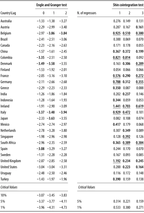
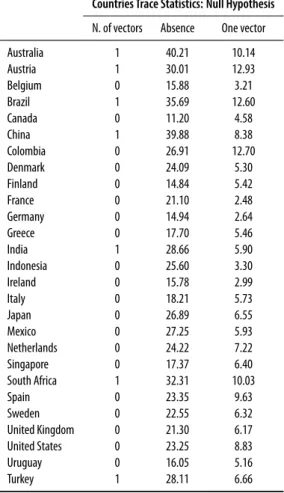
To assess the existence of cointegration between variables, we run the following cointegration tests:Engle and Granger(1987),Shin(1994), andJohansen(1988). The first two tests are univariate whereas the third is multivariate. The null hypothesis of the first test is absence of cointegration and alternative hypothesis is existence of cointegration. Second test is a confirmatory procedure whre the null hypothesis is existence of cointegration and alternative hypothesis is no cointegration. Trace and maximum eigenvalue tests proposed by Johansen if and how many cointegration relationships may exist.
Table 1.Results of univariate cointegration test.
Engle and Granger test Shin cointegration test
Country\Lag 0 1 2 N. of regressors 1 2 3
Australia -1.33 -1.38 -3.27 0.276 0.149 0.131
Austria -2.29 -2.99 -3.40 0.287 0.167 0.161
Belgium -2.97 -3.86 -3.84 0.925 0.510 0.380
Brazil -2.41 -2.51 -3.06 0.300 0.069 0.070
Canada -2.23 -2.16 -2.63 0.171 0.178 0.055
China -1.57 -1.61 -2.45 0.367 0.372 0.199
Colombia -3.35 -2.51 -2.50 0.821 0.814 0.092
Denmark -3.49 -3.58 -3.55 0.163 0.306 0.289
Finland -1.53 -1.92 -2.01 0.054 0.066 0.066
France -2.05 -3.16 -3.10 0.576 0.290 0.272
Germany -2.11 -2.66 -2.68 0.788 0.312 0.355
Greece -2.29 -2.23 -2.33 0.350 0.087 0.088
India -1.26 -1.86 -1.84 0.202 0.237 0.146
Indonesia -1.28 -1.64 -1.93 0.344 0.059 0.053
Ireland -1.91 -2.90 -3.09 1.441 0.703 0.619
Italy -3.37 -3.48 -3.94 0.929 0.472 0.101
Japan -2.33 -3.63 -3.55 0.082 0.108 0.074
Mexico -2.74 -2.74 -2.97 0.417 0.179 0.068
Netherlands -2.78 -3.28 -3.80 0.307 0.349 0.089
Singapore -1.98 -2.96 -2.98 0.128 0.392 0.126
South Africa -2.96 -2.35 -2.59 0.365 0.389 0.384
Spain -3.08 -3.29 -3.27 0.244 0.170 0.070
Sweden -1.31 -2.28 -2.28 0.167 0.093 0.085
United Kingdom -2.87 -2.85 -2.58 1.192 0.234 0.245
United States -3.04 -3.04 -3.31 0.200 0.223 0.164
Uruguay -2.48 -2.50 -2.46 0.116 0.172 0.148
Turkey -1.43 -1.97 -1.96 0.390 0.159 0.138
Critical Values Critical Values
10% -3.07 -3.45 -3.83
5% -3.37 -3.77 -4.11 5% 0.314 0.221 0.159
Table 2.Results of multivariate cointegration test.
Countries Trace Statistics: Null Hypothesis
N. of vectors Absence One vector
Australia 1 40.21 10.14
Austria 1 30.01 12.93
Belgium 0 15.88 3.21
Brazil 1 35.69 12.60
Canada 0 11.20 4.58
China 1 39.88 8.38
Colombia 0 26.91 12.70
Denmark 0 24.09 5.30
Finland 0 14.84 5.42
France 0 21.10 2.48
Germany 0 14.94 2.64
Greece 0 17.70 5.46
India 1 28.66 5.90
Indonesia 0 25.60 3.30
Ireland 0 15.78 2.99
Italy 0 18.21 5.73
Japan 0 26.89 6.55
Mexico 0 27.25 5.93
Netherlands 0 24.22 7.22
Singapore 0 17.37 6.40
South Africa 1 32.31 10.03
Spain 0 23.35 9.63
Sweden 0 22.55 6.32
United Kingdom 0 21.30 6.17
United States 0 23.25 8.83
Uruguay 0 16.05 5.16
Turkey 1 28.11 6.66
The specification may be improved by adding other variables. For example, a variable that controls the possible Balassa–Samuelson effect may alter the results towards finding stronger evidence of cointegration.5
4.3 Is there evidence of global effects?
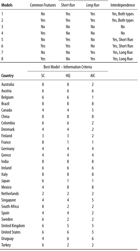
This section attempts to answer the question of whether the model with external factors is better than the model without these factors. We compare eight different specifications. We consider models with complete interdependence, in other words, that have external factors, in the short and long term dynamics, similar to the equation (12). There are models in which interdependence is allowed only in the long term. In another specification, we allow interdependence only on short-term dynamics. Finally, there are models in which no interdependence is allowed. We estimate the models also allowing a structure with or without
5In this study, we could have analyzed a broader set of information using variables to control for the
common cycles.6 We compare these eight models using the Schwarz (SC), Hannan-Quinn
(HQ), and Akaike information criteria (AIC).
Table 3presents a detailed description of the models and all information criteria. Options 3 and 4 consist of models with no interdependence. The evidence in favor of interdependence varies between countries. According to all information criteria, there is no evidence of interdependence for the following countries: Australia, Ireland, India, Netherlands, and Turkey. For other countries, there is evidence of interdependence in the short and/or long term. Thus, we can conclude that statistical evidence corroborates the hypothesis of interdependence for a large group of countries. The next step in the analysis is to assess the relevance of global and domestic factors to exchange rate misalignment estimate.
4.4 Calculating exchange rate misalignment using the GVECM
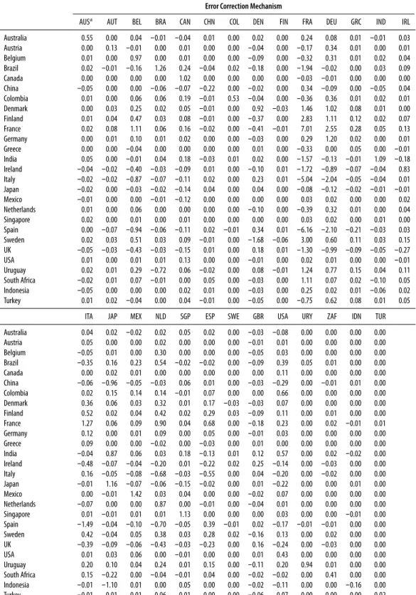
This section describes the results of the GVECM estimation. Table 6shows the estimated cointegrated vectors for each country. Table 4shows the results of the estimate loading factor given by (17) for real exchange rate equation. The value in line 𝑖 and column 𝑗
represents the weight of the error correction mechanism of country 𝑗 that will be used to calculate the misalignment for country 𝑖. For example, we can check that the United States and Germany columns contain many non-zero terms. This suggests strong linkages between these economies and others economies analyzed in the sample. In the case of Germany, there seems to be a strong effect in eurozone countries. Brazil is an example of the opposite case. Here, the Brazilian exchange rate misalignment causes minor effects on all countries other than Uruguay. Although Brazil is a large economy, its global share is relatively small. Intuitively, the Brazilian economy is affected by others countries’ disequilibrium, but its own disequilibrium does not affect others countries. The United States exchange rate misalignment may generate quite small effects on eurozone countries.
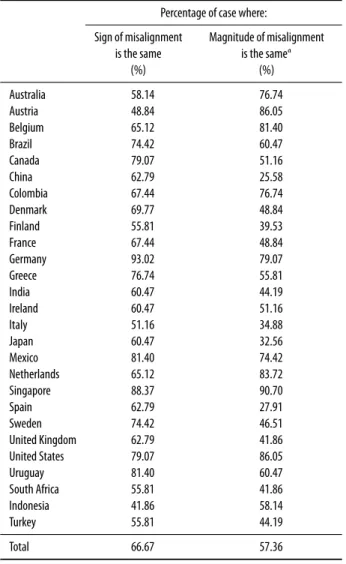
Table 5compares the results of the exchange rate misalignment using the traditional and GVAR methodologies. In general, the estimate misalignment tends to have the same sign for almost 67% of the sample. There are 1,161 (27×43) estimate of exchange rate misalignments, across all countries and periods. For the United States, the results are virtually the same in terms of sign and magnitude. The overall picture does not change when the comparison is made using the magnitude rather than the sign of the exchange rate misalignment. We compute the proportion of each case out of the total, where the estimate misalignments for both models have the same sign and absolute value above 10%, or different signs but absolute an below 10%. In the 57% of cases, these criteria were satisfied. However, in about 43% of cases, the estimates are not the same. The results inTable 5suggest that quite different results can be obtained from the GVAR. The dynamics of real exchange rates in these countries cannot be seen as detached from the rest of world, or at least from their main trading partners.Table 6shows the estimates of all parameters necessary to solve the GVAR.
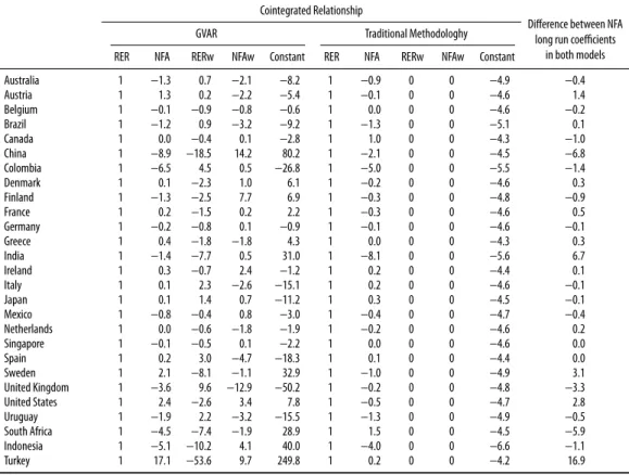
Table 7 provides information about the source of the differences between the two methodologies. First, the coefficient of the NFA variable changes quite significantly for many countries. This may explain part of the change in the results and highlights the importance of investigating the main drivers of real exchange rates in the long run. However, there are countries where the coefficient hardly changes at all, but the external variables cause
6SeeHecq, Palm, and Urbain(2000) andHecq, Palm, and Urbain(2002) for a common cycle definition, a
Table 3.Results of the tests for interdependence.
External Variables in the Model
Models Common Features Short Run Long Run Interdependence
1 No Yes Yes Yes, Both types
2 Yes Yes Yes Yes, Both types
3 No No No No
4 Yes No No No
5 No Yes No Yes, Short Run
6 Yes Yes No Yes, Short Run
7 No No Yes Yes, Long Run
8 Yes No Yes Yes, Long Run
Best Model – Information Criteria
Country SC HQ AIC
Australia 8 8 2
Austria 6 6 6
Belgium 6 6 1
Brazil 8 8 8
Canada 4 4 5
China 8 8 8
Colombia 6 6 2
Denmark 4 4 2
Finland 3 3 2
France 8 1 1
Germany 4 4 4
Greece 4 4 4
India 8 8 8
Ireland 6 6 6
Italy 8 8 8
Japan 6 1 1
Mexico 4 8 8
Netherlands 2 2 2
Singapore 4 4 5
South Africa 8 2 2
Spain 4 4 2
Sweden 6 2 2
United Kingdom 6 5 5
United States 6 6 5
Uruguay 4 6 6
Table 4.Loading factor for calculating exchange rate misalignment from the GVAR model.
Error Correction Mechanism
AUS𝔞 AUT BEL BRA CAN CHN COL DEN FIN FRA DEU GRC IND IRL
Australia 0.55 0.00 0.04 -0.01 -0.04 0.01 0.00 0.02 0.00 0.24 0.08 0.01 -0.01 0.03
Austria 0.00 0.13 -0.01 0.00 0.01 0.00 0.00 -0.04 0.00 -0.17 0.34 0.01 0.00 0.01
Belgium 0.01 0.00 0.97 0.00 0.01 0.00 0.00 -0.09 0.00 -0.32 0.31 0.01 0.02 0.04
Brazil 0.02 -0.01 -0.16 1.26 0.24 -0.04 0.02 -0.18 0.00 -1.94 -0.02 0.00 0.03 0.09
Canada 0.00 0.00 0.00 0.00 1.02 0.00 0.00 0.00 0.00 -0.03 -0.01 0.00 0.00 0.00
China -0.05 0.00 0.00 -0.06 -0.07 -0.22 0.00 -0.02 0.00 0.34 -0.09 0.00 -0.05 0.04
Colombia 0.01 0.00 0.06 0.06 0.19 -0.01 0.53 -0.04 0.00 -0.36 0.36 0.01 0.02 0.01
Denmark 0.00 0.03 0.25 0.02 0.05 -0.01 0.00 0.92 -0.03 1.46 1.02 0.08 0.01 0.00
Finland 0.01 0.04 0.47 0.03 0.08 -0.01 0.00 -0.37 0.00 2.83 1.11 0.12 0.02 0.07
France 0.02 0.08 1.11 0.06 0.16 -0.02 0.00 -0.41 -0.01 7.01 2.55 0.28 0.05 0.13
Germany 0.00 0.01 0.10 0.01 0.02 0.00 0.00 -0.03 0.00 0.29 1.20 0.02 0.00 0.01
Greece 0.00 0.00 -0.04 0.00 0.00 0.00 0.00 0.01 0.00 -0.33 0.00 0.05 0.00 -0.01
India 0.05 0.00 -0.01 0.04 0.18 -0.03 0.01 0.02 0.00 -1.57 -0.13 -0.01 1.09 -0.18
Ireland -0.04 -0.02 -0.40 -0.03 -0.09 0.01 0.00 -0.10 0.01 -1.72 -0.89 -0.07 -0.04 0.83 Italy -0.02 -0.02 -0.87 -0.07 -0.11 0.02 0.00 0.23 0.01 -5.04 -2.04 -0.05 -0.04 0.01 Japan -0.02 0.00 -0.03 -0.02 -0.14 0.04 0.00 0.04 0.00 -0.08 -0.12 -0.02 -0.01 -0.01
Mexico -0.01 0.00 0.00 -0.01 -0.12 0.00 0.00 0.00 0.00 0.03 0.02 0.00 0.00 0.02
Netherlands 0.01 0.00 0.06 0.00 0.00 0.00 0.00 -0.10 0.00 -0.39 0.32 0.01 0.00 0.04
Singapore 0.02 0.00 0.01 0.00 0.01 0.00 0.00 0.00 0.00 0.03 0.02 0.00 0.01 0.00
Spain 0.00 -0.07 -0.94 -0.06 -0.11 0.02 -0.01 0.34 0.01 -6.16 -2.10 -0.21 -0.03 0.03
Sweden 0.02 0.03 0.51 0.03 0.09 -0.01 0.00 -1.68 -0.06 3.00 0.60 0.11 0.03 0.15
UK -0.05 -0.03 -0.43 -0.03 -0.15 0.01 0.00 0.18 0.01 -1.30 -0.99 -0.09 -0.05 -0.27
USA 0.01 0.00 0.01 0.01 0.13 0.00 0.00 -0.01 0.00 0.02 0.01 0.00 0.00 -0.01
Uruguay 0.02 0.01 0.29 -0.72 0.06 -0.02 0.00 0.08 -0.01 1.24 0.77 0.15 0.04 0.11
South Africa -0.02 0.01 0.07 -0.01 0.00 0.05 0.00 -0.03 0.00 1.11 0.07 0.02 -0.10 0.05
Indonesia -0.05 0.00 0.00 0.00 0.02 0.01 0.00 -0.03 0.00 0.25 0.02 0.01 -0.06 0.02
Turkey 0.01 0.02 -0.04 0.00 0.04 -0.01 0.00 -0.05 0.00 -0.75 0.62 0.08 0.01 0.05
ITA JAP MEX NLD SGP ESP SWE GBR USA URY ZAF IDN TUR
Australia 0.04 0.02 -0.02 0.02 0.05 0.02 0.00 -0.03 -0.08 0.00 0.00 0.00 0.00
Austria 0.05 0.00 0.00 0.02 0.00 0.00 0.00 -0.01 0.01 0.00 0.00 0.00 0.00
Belgium -0.05 0.01 0.00 0.30 0.00 0.00 0.00 -0.05 0.03 0.00 0.00 0.00 0.00
Brazil -0.35 0.16 0.23 0.54 -0.02 -0.02 0.00 -0.09 0.39 0.05 0.01 0.00 0.00
Canada 0.00 0.02 0.01 0.00 0.00 0.00 0.00 0.00 0.11 0.00 0.00 0.00 0.00
China -0.06 -0.96 -0.05 -0.03 0.06 0.01 0.00 -0.03 -0.29 0.00 -0.01 0.01 0.00
Colombia 0.02 0.15 0.14 0.14 -0.01 0.07 0.00 0.00 0.66 0.00 0.00 0.00 0.00
Denmark 0.36 0.06 0.03 0.32 0.01 0.17 -0.03 -0.03 0.07 0.00 0.00 0.00 0.00
Finland 0.52 0.02 0.04 0.42 0.02 0.29 0.03 -0.09 0.11 0.00 0.01 0.00 0.00
France 1.27 0.06 0.09 0.90 0.04 0.68 0.00 -0.18 0.23 0.00 0.02 -0.01 0.01
Germany 0.12 0.00 0.01 0.09 0.00 0.05 0.00 -0.01 0.03 0.00 0.00 0.00 0.00
Greece 0.09 0.00 0.00 -0.02 0.00 -0.03 0.00 0.01 0.00 0.00 0.00 0.00 0.00
India -0.04 0.87 0.06 0.03 0.18 -0.13 0.01 0.12 0.57 0.00 0.02 -0.02 0.00
Ireland -0.48 -0.07 -0.04 -0.20 0.01 -0.22 0.02 0.25 -0.14 0.00 -0.03 0.00 0.00 Italy 0.16 -0.05 -0.08 -0.68 -0.03 -0.55 0.00 0.04 -0.20 0.00 -0.02 0.00 0.00
Japan -0.01 1.16 -0.07 -0.06 -0.15 -0.02 0.00 0.01 -0.22 0.00 0.00 0.01 0.00
Mexico 0.00 -0.01 1.42 0.03 0.04 0.00 0.00 -0.02 0.07 0.00 0.00 0.00 0.00
Netherlands -0.07 0.00 0.00 0.87 0.00 -0.01 0.00 -0.04 0.01 0.00 0.00 0.00 0.00
Singapore 0.01 -0.01 0.01 0.01 1.13 0.00 0.00 0.00 0.03 0.00 0.00 -0.01 0.00
Spain -1.49 -0.04 -0.10 -0.70 -0.05 0.39 -0.01 0.02 -0.17 -0.01 -0.01 0.00 0.00
Sweden 0.42 -0.04 0.05 0.38 0.03 0.28 0.02 -0.16 0.13 0.00 0.02 0.00 0.00
UK -0.39 -0.09 -0.06 -0.43 -0.03 -0.23 0.00 0.16 -0.24 0.00 -0.03 0.00 0.00
USA 0.01 0.03 0.06 0.00 -0.01 0.00 0.00 0.01 0.43 0.00 0.00 0.00 0.00
Uruguay 0.20 0.10 0.04 0.24 0.01 0.15 0.00 -0.11 0.20 0.94 0.01 0.00 0.00
South Africa 0.15 -0.22 0.00 -0.04 -0.01 0.04 0.00 -0.02 -0.02 0.00 0.41 0.00 0.00 Indonesia -0.01 -1.10 0.01 0.00 0.05 0.00 0.00 -0.02 -0.11 0.00 0.00 -0.16 0.00
Turkey -0.01 0.01 0.01 0.06 0.01 0.00 0.00 -0.06 0.07 0.00 0.00 0.00 0.02
𝔞ISO alpha-3 country codes: AUS (Australia), AUT (Austria), BEL (Belgium), BRA (Brazil), CAN (Canada), CHN (China), COL (Colombia),
Table 5.Comparing exchanges rate misalignment estimates.
Percentage of case where:
Sign of misalignment is the same
(%)
Magnitude of misalignment is the same𝔞
(%)
Australia 58.14 76.74
Austria 48.84 86.05
Belgium 65.12 81.40
Brazil 74.42 60.47
Canada 79.07 51.16
China 62.79 25.58
Colombia 67.44 76.74
Denmark 69.77 48.84
Finland 55.81 39.53
France 67.44 48.84
Germany 93.02 79.07
Greece 76.74 55.81
India 60.47 44.19
Ireland 60.47 51.16
Italy 51.16 34.88
Japan 60.47 32.56
Mexico 81.40 74.42
Netherlands 65.12 83.72
Singapore 88.37 90.70
Spain 62.79 27.91
Sweden 74.42 46.51
United Kingdom 62.79 41.86
United States 79.07 86.05
Uruguay 81.40 60.47
South Africa 55.81 41.86
Indonesia 41.86 58.14
Turkey 55.81 44.19
Total 66.67 57.36
𝔞If both estimates give a value of misalignment above 10% in modulus or
below 10% in modulus simultaneously.
changes in the magnitude of the exchange misalignment estimate. Brazil is a good example. Although there is a minor change in the NFA coefficient when external variables are included in the model, they add relevant information to the long run level of the exchange rate. The misalignment of the exchange rate for both models is different after introducing foreign variables.
Table 6.Coefficient estimates for each country model used to solve the GVAR.
Loading Matrix Cointegrated Vectors Contemporaneous Effect
Country 𝛼𝑖1 𝛼𝑖2 𝛽𝑖,RER 𝛽𝑖,NFA 𝛽𝑖,RERw 𝛽𝑖,NFAw 𝛽𝑖,Constant 𝐶𝑖,11 𝐶𝑖,12 𝐶𝑖,21 𝐶𝑖,22
Australia −0.45 0.27 1 −1.34 0.71 −2.07 −8.21 −0.55 0.55 0.54 −0.66
Austria −0.07 −0.37 1 1.31 0.23 −2.25 −5.43 0.90 −0.10 −0.04 0.06
Belgium −0.39 −0.03 1 −0.13 −0.86 −0.77 −0.60 1.11 −0.23 −0.29 0.47
Brazil −0.89 −0.18 1 −1.19 0.85 −3.21 −9.18 −0.25 2.74 0.82 −0.44
Canada −0.16 −0.03 1 0.00 −0.37 0.11 −2.79 −0.02 1.22 0.10 −0.49
China 0.06 0.04 1 −8.88 −18.54 14.25 80.15 0.42 0.10 −0.39 0.41
Colombia −0.08 0.01 1 −6.45 4.47 0.48 −26.80 0.39 1.58 0.10 −0.14
Denmark −0.05 0.29 1 0.10 −2.26 1.03 6.12 −0.01 0.46 −1.09 −0.78
Finland 0.00 0.41 1 −1.27 −2.48 7.74 6.92 0.62 0.47 0.41 5.56
France −0.82 0.59 1 0.18 −1.49 0.18 2.24 1.15 −0.62 0.42 −0.52
Germany −0.45 −0.18 1 −0.15 −0.80 0.14 −0.89 0.52 −0.96 0.33 0.15
Greece 0.00 −0.31 1 0.36 −1.84 −1.81 4.28 0.61 −0.25 −0.49 −0.69
India −0.32 −0.03 1 −1.42 −7.74 0.49 31.01 1.87 0.63 0.09 −0.27
Ireland −0.52 0.17 1 0.30 −0.68 2.44 −1.19 −0.44 −0.90 0.75 −4.21
Italy −0.46 0.14 1 0.09 2.25 −2.56 −15.09 −0.17 0.62 −0.39 −0.01
Japan −0.48 −0.11 1 0.14 1.41 0.70 −11.19 −1.36 −1.91 −0.19 −0.53
Mexico −1.05 −0.40 1 −0.83 −0.41 0.84 −2.95 0.98 0.42 0.06 −0.13
Netherlands −0.21 −0.55 1 0.00 −0.56 −1.85 −1.94 1.33 −0.05 −1.37 1.72
Singapore −0.20 −0.45 1 −0.05 −0.51 0.08 −2.19 0.64 0.24 −0.80 −2.65
Spain −0.36 −0.17 1 0.16 2.97 −4.67 −18.32 0.29 0.82 −0.88 1.40
Sweden −0.04 −0.27 1 2.07 −8.08 −1.09 32.92 0.59 −0.23 2.26 0.13
UK −0.04 0.09 1 −3.56 9.64 −12.90 −50.20 −2.27 1.22 −0.10 −2.19
USA −0.12 −0.06 1 2.35 −2.59 3.40 7.75 −0.25 0.46 0.59 −0.68
Uruguay −0.42 0.02 1 −1.85 2.16 −3.16 −15.47 −0.60 −0.53 0.09 1.19
South Africa −0.41 0.14 1 −4.45 −7.39 −1.89 28.86 1.98 −3.85 −0.72 −0.32
Indonesia 0.05 0.07 1 −5.11 −10.19 4.05 39.97 −1.60 −0.59 −1.94 −3.51
Turkey −0.02 −0.05 1 17.13 −53.64 9.75 249.77 1.10 0.88 1.42 −1.75
Table 7.Comparing the cointegrated coefficient of the GVAR and traditional methodologies.
Cointegrated Relationship
Difference between NFA long run coefficients
in both models
GVAR Traditional Methodologhy
RER NFA RERw NFAw Constant RER NFA RERw NFAw Constant
Australia 1 −1.3 0.7 −2.1 −8.2 1 −0.9 0 0 −4.9 −0.4
Austria 1 1.3 0.2 −2.2 −5.4 1 −0.1 0 0 −4.6 1.4
Belgium 1 −0.1 −0.9 −0.8 −0.6 1 0.0 0 0 −4.6 −0.2
Brazil 1 −1.2 0.9 −3.2 −9.2 1 −1.3 0 0 −5.1 0.1
Canada 1 0.0 −0.4 0.1 −2.8 1 1.0 0 0 −4.3 −1.0
China 1 −8.9 −18.5 14.2 80.2 1 −2.1 0 0 −4.5 −6.8
Colombia 1 −6.5 4.5 0.5 −26.8 1 −5.0 0 0 −5.5 −1.4
Denmark 1 0.1 −2.3 1.0 6.1 1 −0.2 0 0 −4.6 0.3
Finland 1 −1.3 −2.5 7.7 6.9 1 −0.3 0 0 −4.8 −0.9
France 1 0.2 −1.5 0.2 2.2 1 −0.3 0 0 −4.6 0.5
Germany 1 −0.2 −0.8 0.1 −0.9 1 −0.1 0 0 −4.6 −0.1
Greece 1 0.4 −1.8 −1.8 4.3 1 0.0 0 0 −4.3 0.3
India 1 −1.4 −7.7 0.5 31.0 1 −8.1 0 0 −5.6 6.7
Ireland 1 0.3 −0.7 2.4 −1.2 1 0.2 0 0 −4.4 0.1
Italy 1 0.1 2.3 −2.6 −15.1 1 0.2 0 0 −4.6 −0.1
Japan 1 0.1 1.4 0.7 −11.2 1 0.3 0 0 −4.5 −0.1
Mexico 1 −0.8 −0.4 0.8 −3.0 1 −0.4 0 0 −4.7 −0.4
Netherlands 1 0.0 −0.6 −1.8 −1.9 1 −0.2 0 0 −4.6 0.2
Singapore 1 −0.1 −0.5 0.1 −2.2 1 0.0 0 0 −4.6 0.0
Spain 1 0.2 3.0 −4.7 −18.3 1 0.1 0 0 −4.4 0.0
Sweden 1 2.1 −8.1 −1.1 32.9 1 −1.0 0 0 −4.9 3.1
United Kingdom 1 −3.6 9.6 −12.9 −50.2 1 −0.2 0 0 −4.8 −3.3
United States 1 2.4 −2.6 3.4 7.8 1 −0.5 0 0 −4.7 2.8
Uruguay 1 −1.9 2.2 −3.2 −15.5 1 −1.3 0 0 −4.9 −0.5
South Africa 1 −4.5 −7.4 −1.9 28.9 1 1.5 0 0 −4.5 −5.9
Indonesia 1 −5.1 −10.2 4.1 40.0 1 −4.0 0 0 −6.6 −1.1
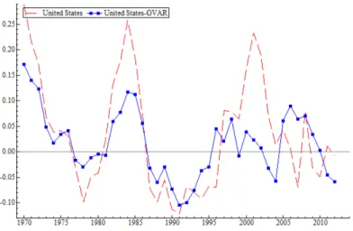
Figure 1.Real exchange rate misalignment estimate – GVAR versus traditional methodology – United States.
Figure 2.Real exchange rate misalignment estimate – GVAR versus traditional methodology – Brazil.
In a recent paper,Ericsson and Reisman(2012) proposes a refinement of the GVAR approach using a model selection procedure calledAutometrics.7 This refinement allows one
to search for points of instability and structural changes in the modeling process. It is also possible to incorporate a wider range of information sets in each country model. However, this must occur within a rigorous general-to-specific econometric modeling approach in the spirit of the London School of Economics (LSE) tradition developed by David Hendry. This reduces the possibility of criticism that a time series analysis can only manage a few real exchange rate determinants at a time, as compared to panel models. By using the GVAR refinement proposed byEricsson and Reisman(2012), it is possible, for example, to match the merits of the IMF approach, with its wide range of variables, to a panel with the merits of a global model. One can opt to model different set fundamentals for each country.
The interdependence among countries is introduced in GVAR by adding trade weighted foreign variables in the model of each specific country. We opt to useAutometricssearch algorithm to check if these variables explain the dynamics of each country models. The traditional methodology can be extended in many directions. The GVAR is one possible way but not the only one. We decide to construct indicators functions (impulse, step and time trend dummies) to allow for structural change in mean of the process. We also run principal components analysis on all first differences of the logarithm of real effective exchange rate and net foreign assets and use the factors as possible regressors. The rationality for this relies on possible existence of another global factor not well captured by GVAR averages variables.
In order to evaluate the GVAR we must compare it to a more general model. We opt to include others sources of interdependence and structural change in the mean parameters of the model. This general model nests the GVAR structure. We run theAutometricsin two steps.
In the first step the general unrestricted model (GUM) is given by the following equation:
Δ𝑥𝑖,𝑡=∑𝑞 ℎ=1
𝜃1
1ℎ𝑉ℎ𝑡𝑖 +
𝑇𝑖
∑ ℎ=1
𝜃1
2ℎIS(𝑇ℎ) +
𝑇𝑖
∑ ℎ=1
𝜃1
2ℎDS(𝑇ℎ) +
𝑇𝑖
∑ 𝑖=1
𝜃1
3ℎDT(𝑇ℎ) + 𝑢1𝑖, (19)
where
IS(𝑇𝑖) = {1,
if 𝑡 = 𝑇𝑖,
0, if 𝑡 ≠ 𝑇𝑖; DS(𝑇𝑖) ={1,
if 𝑡 ≥ 𝑇𝑖,
0, if 𝑡 < 𝑇𝑖; DT(𝑇𝑖) ={𝑡,
if 𝑡 ≥ 𝑇𝑖,
0, if 𝑡 < 𝑇𝑖;
and𝑉𝑖= 𝑉1𝑖, 𝑉2𝑖, … , 𝑉𝑞𝑖contains all GVAR’s country𝑖variables. The superscript denotes
the step.
In the second step the general unrestricted model contains the variables of the final model in the first step and broader set of variables:
Δ𝑥𝑖,𝑡= 𝑞 ∑
ℎ=1𝜃
2
1𝑖FM𝑖𝑡+
𝑁 ∑ ℎ=1 𝑘𝑖 ∑ 𝑗=1𝜃 2
2𝑖𝑗Δ𝑥ℎ,𝑡−𝑗+
𝑁 ∑ ℎ=1 𝑘𝑖 ∑ 𝑗=1𝜃 2
3𝑖𝑗Δ𝑥∗ℎ,𝑡−𝑗
+ ∑𝑁 ℎ=1,ℎ≠𝑗
𝜃2
4𝑖𝑗ecmℎ,𝑡−1+
2∗𝑁 ∑ ℎ=1 𝑘𝑖 ∑ 𝑗=1 𝜃2
3𝑖𝑗PCℎ,𝑡−𝑗+ 𝑢2𝑖, (20)
whereFM denotes the variables in the final model of step 1 andPCdenotes the principal components of all RER and NFA variables,ecmdenotes error correction mechanism and the remainder variables were defined previously in the paper.
The GUM of the first step in our exercise contains a total of TOT1= 𝑇 ∗3+2∗6+2+1
variables. In our application TOT1 equals 75 = 30 ∗ 3 + 12 + 2 + 1. The GUM in the second step will contain at least TOT2variables (2 ∗ [𝑁 + (𝑁 − 1)] + 2 ∗ [𝑁 + (𝑁 − 1)] + (𝑁 − 1) + 2 ∗ 𝑁). In our example the number of countries is 27 and TOT2equals 292. The GUM upper limit will be292 + 75 = 367. TheAutometricswill retain under the null that all coefficients are zero an average of irrelevant regressors given by TOT = (TOT1+TOT2)
Autometrics allows us to check whether the GVAR approach is a congruent statistical model and a rival model that contains broader information set can encompass the GVAR. If the final model contains only the variables of the traditional approach it is reasonable to conclude that neither GVAR nor the broader GUM are worth taking.
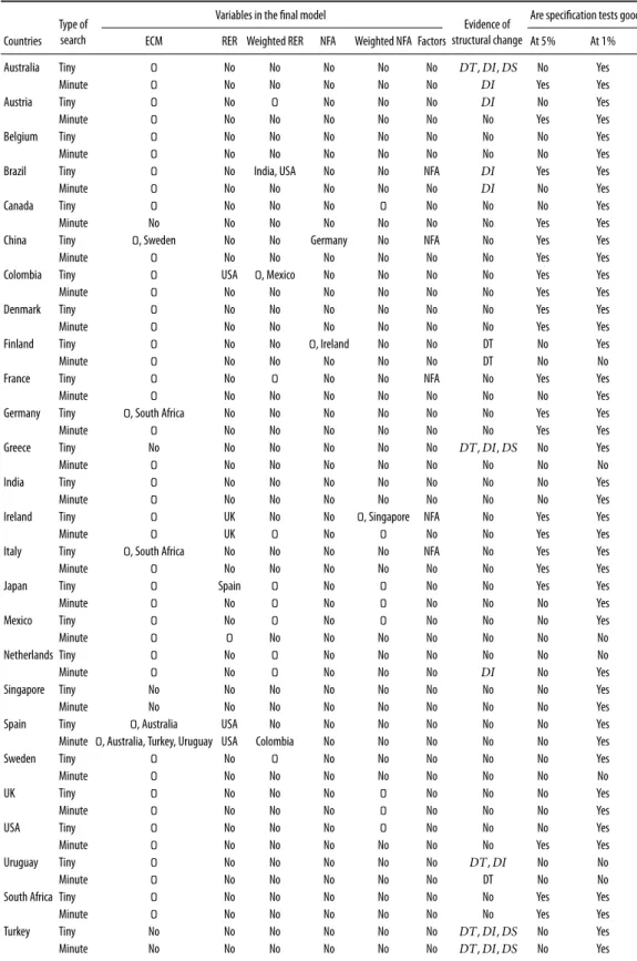
Table 8provides information on each country final model chosen byAutometricssearch algorithm. In some case there is evidence of structural change (e.g. Australia, Greece, Uruguay, Turkey). In these cases, a closer look to other domestic variables can be an alternative. For some countries our evidence suggests that the GVAR can not capture all possible sources of interdependence. For example, in the case of Ireland, a closer link to the dynamics of United Kingdom’s real effective exchange was revealed. However the foreign NFA weigthed variable seems to explain the dynamics in United Kingdom and United States cases quite well. These countries have the leading financial centers of the world, and GVAR is probably capturing this interdependence channel. In many countries the final model selected byAutometricscontains the foreign trade weighted variable. This results suggest that GVAR improves of our understanding on the dynamics real exchange rate and net foreign asset. The principal components variables were selected only in some few models. For some countries, the results ofAutometricsusing minute instead of tiny significance level seems more intuitive (e.g. Brazil or Germany). Spain is the only country thatAutometrics results are not easy to rationalize.
4.5 Discussion, limitations and possible extensions
The previous discussion on the merits and limitations of the time series and panel approaches is addressed in this section, as well as whether the GVAR model can be a bridge linking both approaches. The time series approaches allow little room to introduce fundamentals because of the sample size available in macroeconomic datasets. The panel approach allows a more flexible structure and the inclusion of a larger group of fundamentals in the analysis. However, this approach must limit heterogeneity to a manageable level. It is not clear to what extent this can lead to distortions, since the main goal is to make assertions on specific units, not to assess the relevance of a group of variables in explaining real exchange rate movements and their average effect. A GVAR model can reconcile the merits of the two approaches, allowing us to map directly the effect of trading partner shocks on a country.
In the same way, it is possible to adapt the decomposition ofGonzalo and Granger(1995) to the GVAR environment. The same can be done for a Beveridge and Nelson decomposition, as shown in the work ofProietti(1997), under a VECM framework. The development of a model for the eurozone is a natural extension of our work. A regional factor can be easily added to the GVAR to map directly the interdependence between countries in the region. To the best of our knowledge, this has not been done before. Although we did not do so, our GVAR model was able to capture a strong interdependence effect among eurozone countries.
Even the IMF approach does not directly tackle the question of interdependence between countries. However, the IMF approach does have the benefit of considering a wide range of fundamentals, and incorporates the role of policy gaps in determining the misalignment.
5. Final remarks
Table 8.Summary of Autometrics results.
Type of search
Variables in the final model
Evidence of structural change
Are specification tests good?
Countries ECM RER Weighted RER NFA Weighted NFA Factors At 5% At 1%
Australia Tiny O No No No No No DT,DI,DS No Yes
Minute O No No No No No DI Yes Yes
Austria Tiny O No O No No No DI No Yes
Minute O No No No No No No Yes Yes
Belgium Tiny O No No No No No No No Yes
Minute O No No No No No No No Yes
Brazil Tiny O No India, USA No No NFA DI Yes Yes
Minute O No No No No No DI No Yes
Canada Tiny O No No No O No No No Yes
Minute No No No No No No No Yes Yes
China Tiny O, Sweden No No Germany No NFA No Yes Yes
Minute O No No No No No No Yes Yes
Colombia Tiny O USA O, Mexico No No No No Yes Yes
Minute O No No No No No No Yes Yes
Denmark Tiny O No No No No No No Yes Yes
Minute O No No No No No No Yes Yes
Finland Tiny O No No O, Ireland No No DT No Yes
Minute O No No No No No DT No No
France Tiny O No O No No NFA No Yes Yes
Minute O No No No No No No No Yes
Germany Tiny O, South Africa No No No No No No Yes Yes
Minute O No No No No No No Yes Yes
Greece Tiny No No No No No No DT,DI,DS No Yes
Minute O No No No No No No No No
India Tiny O No No No No No No No Yes
Minute O No No No No No No No Yes
Ireland Tiny O UK No No O, Singapore NFA No Yes Yes
Minute O UK O No O No No Yes Yes
Italy Tiny O, South Africa No No No No NFA No Yes Yes
Minute O No No No No No No Yes Yes
Japan Tiny O Spain O No O No No Yes Yes
Minute O No O No O No No No Yes
Mexico Tiny O No O No O No No No Yes
Minute O O No No No No No No No
Netherlands Tiny O No O No No No No No No
Minute O No O No No No DI No Yes
Singapore Tiny No No No No No No No No Yes
Minute No No No No No No No No Yes
Spain Tiny O, Australia USA No No No No No No Yes
Minute O, Australia, Turkey, Uruguay USA Colombia No No No No No Yes
Sweden Tiny O No O No No No No No Yes
Minute O No No No No No No No No
UK Tiny O No No No O No No No Yes
Minute O No No No O No No No Yes
USA Tiny O No No No O No No No Yes
Minute O No No No No No No Yes Yes
Uruguay Tiny O No No No No No DT,DI No No
Minute O No No No No No DT No No
South Africa Tiny O No No No No No No Yes Yes
Minute O No No No No No No Yes Yes
Turkey Tiny No No No No No No DT,DI,DS No Yes
Minute No No No No No No DT,DI,DS No Yes
able to find evidence in favor of interdependence in both the short and long run for some countries. In only a few cases in the sample could the null hypothesis of no interdependence not be rejected.
We also discussed the impact that the GVAR may have on exchange rate misalignment estimates. Here, we adapted the Gonzalo and Granger decomposition to a GVAR framework and conducted an empirical exercise to try to explain the relevance of global effects to exchange rate misalignment estimates. Our findings show that the effects are greater for small or developing countries, because they tend to be more affected by global economy conditions.
Our global model was also capable of detecting important linkages between eurozone countries, as expected. The United States and Germany, two leading economies in the world, seem to have an effect on the real exchange rate of other countries. However, their exchange rate misalignment estimates are only marginally affected in terms of magnitude and sign when both models’ estimates are compared. The reason for this has to do with the dynamics of their real effective exchange rates, which are almost not affected by others countries’ variables.
Finally, possible extensions to our approach include improving on country-specific models by using recent advances in time series model selection to investigate the role of a broader set of domestic variables. We can access not only the statistical significance of external factors but their relative importance in relation to domestic factors.
References
Ahmad, Y., & Craighead, W. D. (2011). Temporal aggregation and purchasing power parity
persistence.Journal of International Money and Finance,30(5), 817–830.
http://dx.doi.org/10.1016/j.jimonfin.2011.05.008
Alberola, E., Cervero, S. G., Lopez, H., & Ubide, A. (1999). Global
equilib-rium exchange rate: Euro, dolar, “ins”, “outs,” and other major currencies in a panel cointegration framework (IMF Working paper No. 175). International
Mone-tary Fund. https://www.imf.org/en/Publications/WP/Issues/2016/12/30/Global-Equilibrium
-Exchange-Rates-Euro-Dollar-Ins-Outs-and-Other-Major-Currencies-in-a-Panel-3369
Bilson, J. F. O. (1979). Recent developments in monetary models of exchange rate determination. Staff Papers (International Monetary Fund),26(2), 201–223.
http://dx.doi.org/10.2307/3866509
Cline, W. R., & Williamson, J. (2008). Estimates of the equilibrium exchange rate of the renminbi:
Is there a consensus and if not, why not? In M. Goldstein & N. R. Lardy (Eds.),Debating
China’s exchange rate policy (pp. 131–168). Peterson Institute for International Economics.
https://piie.com/publications/chapters_preview/4150/04iie4150.pdf
Doornik, J. A. (2009). Autometrics. In J. L. Castle & N. Shephard (Eds.),The methodology and
practice of econometrics: A Festschrift in honour of David F. Hendry.Oxford University Press.
Dornbusch, R. (1976). Expectations and exchange rate dynamics. Journal of Political Economy,
84(6), 1161–1176.https://www.jstor.org/stable/1831272
Edwards, S. (1989). Exchange rate misalignment in developing countries.The World Bank Research
Observer, 4(1), 3–21. http://documents.worldbank.org/curated/en/737331468739271547/ Exchange-rate-misalignment-in-developing-countries
Edwards, S. (1991).Real exchange rates, devaluation, and adjustment: Exchange rate in developing
Engle, R. F., & Granger, C. W. J. (1987). Co-integration and error correction: Representation,
estimation, and testing.Econometrica,55(2), 251–276. http://dx.doi.org/10.2307/1913236
Engle, R. F., Hendry, D. F., & Richard, J.-F. (1983). Exogeneity.Econometrica,51(2), 277–304.
http://dx.doi.org/10.2307/1911990
Ericsson, N. R., & Reisman, E. L. (2012). Evaluating a global vector autoregression for forecasting. International Advances in Economic Research,18(3), 247–258.
http://dx.doi.org/10.1007/s11294-012-9357-0
Faruqee, H. (1995). Long-run determinants of the real exchange rate: A stock-flow perspective. IMF Staff Papers,42(1), 80–107. http://dx.doi.org/10.2307/3867341
Froot, K. A., & Rogoff, K. (1995). Perspectives on PPP and long-run real exchange rates. In
G.M.Grossman&K.Rogoff(Eds.),Handbookofinternationaleconomics(Vol.3,pp.1647–1688).
North Holland.
Ghysels, E., & Miller, I. J. (2015). Testing for cointegration with temporally aggregated and
mixed-frequency time series.Journal of Time Series Analysis,36(6), 797–816.
http://dx.doi.org/10.1111/jtsa.12129
Gonzalo, J.,&Granger, C. (1995). Estimationofcommonlong-memorycomponentsincointegrated
systems.Journal of Business & Economic Statistics,13(1), 27–35.
http://dx.doi.org/10.2307/1392518
Hecq, A., Palm, F. C., & Urbain, J.-P. (2000). Permanent-transitory decomposition in VAR models
with cointegration and common cycles. Oxford Bulletin of Economics and Statistics,62(4),
511–532. http://dx.doi.org/10.1111/1468-0084.00185
Hecq, A., Palm, F. C., & Urbain, J.-P. (2002). Separation, weak exogeneity, and P-T decomposition
in cointegrated VAR systems with common features.Econometric Reviews,21(3), 273–307.
http://dx.doi.org/10.1081/ETC-120015785
Hendry, D. F. (1995). Dynamic econometrics. Oxford University Press.
Hossfeld, O. (2010). Equilibrium real exchange rates and real exchange rate misaligments: Time
series vs. panel estimates(Tech. Rep. No. 65). FIW – Forschungsschwerpunkt Internationale
Wirtschaft.http://hdl.handle.net/10419/121070 (Working Paper)
IMF – International Monetary Fund. (2013). 2013 pilot external sector report. Washington,
DC:InternationalMonetaryFund.https://www.imf.org/en/Publications/Policy-Papers/Issues/
2016/12/31/2013-Pilot-External-Sector-Report-PP4789
Johansen, S. (1988). Statistical analysis of cointegration vectors. Journal of Economic Dynamics
and Control,12(2-3), 231–254. http://dx.doi.org/10.1016/0165-1889(88)90041-3
Johansen, S. (1995). Identifying restrictions of linear equations with applications to simultaneous
equations and cointegration.Journal of Econometrics,69(1), 111–132.
http://dx.doi.org/10.1016/0304-4076(94)01664-L
Kubota, M. (2009).Real exchange rate misaligments(PhD Thesis). University of York, York, North
Yorkshire.
Lane, P. R., & Milesi-Ferretti, G. M. (2007). The external wealth of nations mark II: Revised
and extended estimates of foreign assets and liabilities, 1970–2004. Journal of International
Economics,73(2), 223–250. http://dx.doi.org/10.1016/j.jinteco.2007.02.003
Meese, R. A., & Rogoff, K. (1983). Empirical exchange rate models of the seventies: Do they fit out
of sample? Journal of International Economics,14(1-2), 3–24.
http://dx.doi.org/10.1016/0022-1996(83)90017-X
Mussa, M. (1976). The exchange rate, the balance of payments and monetary and fiscal policy
under a regime of controlled floating.The Scandinavian Journal of Economics,78(2), 229–248.
Pesaran, H. M., Schuermann, T., & Weiner, S. M. (2004). Modeling regional interdependencies
using a global error-correcting macroeconometric model. Journal of Business & Economic
Statistics,22(2), 129–162. http://dx.doi.org/10.1198/073500104000000019
Proietti, T. (1997). Short-run dynamics in cointegrated systems.Oxford Bulletin of Economics and
Statistics,59(3), 405–422. http://dx.doi.org/10.1111/1468-0084.00073
Rossi, B. (2013). Exchange rate predictability.Journal of Economic Literature,51(4), 1063–1119.
http://dx.doi.org/10.1257/jel.51.4.1063
Shin, Y. (1994). A residual-based test of the null of cointegration against the alternative of no
cointegration.Econometric Theory,10(1), 91–115.
http://dx.doi.org/10.1017/S0266466600008240
Stein, J. L. (1995). The fundamental determinants of the real exchange rate of the U.S. dollar
relative to other G-7 currencies(IMF Working Paper No. 95/81). International Monetary Fund.
https://papers.ssrn.com/sol3/papers.cfm?abstract_id=883229
Taylor, A. M. (2001). Potential pitfalls for the purchasing-power-parity puzzle? Sampling and
specification biases in mean-reversion tests of the Law of One Price. Econometrica, 69(2),
473–498. https://www.jstor.org/stable/2692239
Williamson, J. (Ed.). (1994). Estimating equilibrium exchange rates. Peterson Institute for