Braz. J. Phys. vol.39 número1

On a possible connection between Chandler wobble and dark matter

Oyanarte Portilho∗

Instituto de F´ısica, Universidade de Bras´ılia, 70919-970 Bras´ılia–DF, Brazil

(Received on 17 july, 2007)

Chandler wobble excitation and damping, one of the open problems in geophysics, is treated as a consequence in part of the interaction between Earth and a hypothetical oblate ellipsoid made of dark matter. The physical and geometrical parameters of such an ellipsoid and the interacting torque strength is calculated in such a way to reproduce the Chandler wobble component of the polar motion in several epochs, available in the literature. It is also examined the consequences upon the geomagnetic field dynamo and generation of heat in the Earth outer core.

Keywords: Chandler wobble; Polar motion; Dark matter.

1. INTRODUCTION

A 305-day Earth free precession was predicted by Euler in the 18th century and was sought since then by astronomers in the form of small latitude variations. F. K¨ustner in 1888 and S. C. Chandler in 1891 detected such a motion but with a pe-riod of approximately 435 days. Later it was shown by Love [1] and Larmor [2] that such a disagreement between theory and observation is in part consequence of elastic deformation of the Earth which was not considered by the Euler rigid body model (see Smith and Dahlen [3] for further corrections expla-nation). The so called Chandler wobble (CW) is actually one of the major components of the Earth polar motion, together with the annual wobble (AW) which has period of nearly 365 days. The composition of the two wobbles results in a motion with period of around 6.2 years due to the beat phenomenon. The ever increasing measurement precision, for which tech-niques like very long baseline interferometry (VLBI), global positioning system (GPS) and lunar laser ranging (LLR) are employed today, has lead to the conclusion that both wobbles have varying amplitudes. For AW, this may be attributed to seasonal displacement of atmospheric and water masses. On the other hand, excitation and damping of the Chandler wob-ble has become a puzzle to investigators. Several mechanisms have been proposed for its excitation like snow, hidrological, atmospheric and oceanic mass displacements, and large earth-quakes, with defenders and opponents arguing for and against repeatedly and, in view of the large energy involved, the prob-lem is still an open question. In more recent papers, Gross [4] attributes the excitation to ocean bottom pressure variations and changes in ocean currents due to winds while Seitzet al. [5] focus on combined effects due to atmospheric and oceanic causes.

Since it is believed that dark matter (DM) and dark energy composes around 96% of the mass of the Universe we investi-gate in this paper the possibility of DM to contribute, at least in part, for the excitation and damping of Chandler wobble. The effect of DM upon regular matter has been considered mainly on galactic-scale although more recently some authors have studied smaller scale effects. For instance, Froggatt and Nielsen [6]) have investigated the possibility of star-scale ef-fects due to small DM balls; Fr`ereet al. [7] studied the

pres-∗_{Electronic address:portilho@fis.unb.br}

ence of a DM halo centered in the Sun and its influence upon the motion of planets; numerical simulations due to Diemand et al. [8] show the presence of DM clumps surviving near the solar circle; Adler [9] suggests that internal heat produc-tion in Neptune and hot-Jupiter exoplanets is due to accreproduc-tion of planet-bound, not self-annihilating DM. Although the na-ture of the particles that form DM is not known precisely (see for instance Khalil and Mu˜noz [10]) we assume that, as usual, those particles do not interact with regular matter through elec-tromagnetic force but only gravitationally. Furthermore, we speculate that they can interact with each other in such a way to set up an oblate (due to rotation) ellipsoid that might be present inside Earth, occupying the same space without violat-ing any physical law. It can be shown that such an ellipsoid, made of self-interacting DM (otherwise such a structure would not be possible), would be attached to Earth through a spring-like restoring force. In this line, excitation and damping of CW could be, at least partially, consequence of energy exchange between the two bodies, associated to the restoring torque be-tween them. The model does not consider the other known sources for the process nor the Earth internal structure, what are of course over simplifications. However this becomes pos-sible a simple starting point for the calculations, to be sophis-ticated in a later step. H¨opfner [11, 12] has managed to iso-late the CW and AW components from available polar motion data. Our goal is to reproduce H¨opfner’s results for Chandler wobble in various epochs by adjusting the unknown physical and geometrical parameters of the dark matter ellipsoid. For this purpose, we describe both body motion by solving numer-ically the set of differential equations that emerge from Euler equations and demonstrate that CW can be reproduced in such manner. This is explained in the next section while results and discussion are presented in section III.

2. THE MODEL

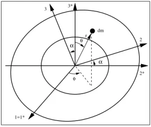
We start by calculating the torque that arises when the polar principal axes 3 and 3∗of two oblate ellipsoids with isotropic densities interacting through the gravitational force are tilted by an angleα (see Fig. 1). The gravitational potential at a point outside the internal ellipsoid (seee. g. Stacey [13]) is given by

V(r,θ)≈ −GM

∗

r +

G r3(C

∗_−A∗_)P

dm

α

α

1=1*

3* 3

2* 2

θ

φ

r

FIG. 1: Two ellipsoids tilted by an angleαaround the common equa-torial principal axes 1 and 1∗. The spherical coordinates (r, θ, φ) that give the position of an infinitesimal massdmwith respect to the 1∗2∗3∗reference frame are also shown.

neglecting higher order terms. HereM∗, A∗ andC∗ are the mass, equatorial and polar momenta of inertia of the internal ellipsoid, respectively, andP2(cosθ) = (3 cos2θ−1)/2 is the Legendre polynomial of second order. The torque over an in-finitesimal massdmlocated at that point is then

dτ=−dm∂V ∂θ =

3G(C∗−A∗)

2r3 sin(2θ)dm. (2) and is directed orthogonal to the plane formed by the polar principal axis 3∗and the positionrofdm(see Fig. 1).

Con-sidering the Earth tilted by an angleαaround the 1-axis (Fig. 1) with respect to the internal ellipsoid it suffers therefore a torque given by the integral

τ= Z

sinφdτ (3)

directed towards the identical axes 1 and 1∗, as projected by the presence of sinφin this integral. The integration should in principle be performed over the entire Earth volume. However considering the Earth density as isotropic, as it is done in the Preliminary Reference Earth Model - PREM (Dziewonski and Anderson [14]), it can be shown that the spherical volume in-ternal to the Earth with radius the same as the polar radius does not contribute to the integral. Therefore the integration overr ranges fromRp, the polar radius, to the radius of the geoid at

a given direction. On the other hand, it is well known (see, for instance, Stacey [13]) that the equation of the geoid is written in the first order approximation in terms of the co-latitudeθ′_as

rg≈a(1−fcos2θ′), (4)

whereais the equatorial radius andf=1−Rp/ais the

flatten-ing. Let us write above equation for the case where the geoid is tilted by an angleαaround the 1-axis (Fig. 1), which yields

rg≈a

1−f(cosαcosθ−sinαsinθsinφ)2

, (5)

whereφ, together with co-latitudeθ, is part of the spherical co-ordinates in the 1∗2∗3∗reference frame. Therefore the torque given by equation (3) becomes

τ = 3 2ρG(C

∗_−A∗₎Z π

0

dθsin(2θ)sinθ ×

Z 2π

0

dφsinφln

_a

Rp

1−f(cosαcosθ−sinαsinθsinφ)2

, (6)

whereρis the average Earth mass density in that region, taken as 2600 kg/m3[14]. Considering that f =1/298.257<<1, we can use the approximation ln(1+x)≈x, obtaining

τ=c1sin(2α), (7)

with c1= 4π₅ρG(C∗−A∗)f. Notice that this is a restoring torque whenα is around 90◦, which gives the stable angular position if no initial angular momenta were involved.

We describe the Earth-ellipsoid motion by the Euler equa-tions

Aω˙1+ (C−A)ω2ω3=τ1 (8)

Aω˙2−(C−A)ω1ω3=τ2 (9)

Cω˙3=τ3=0 ⇒ ω3=constant (10)

A∗ω˙∗1∗+ (C∗−A∗)ω∗₂∗ω∗₃∗ =τ∗₁ (11) A∗ω˙∗₂∗−(C∗−A∗)ω∗₁∗ω∗₃∗ =τ∗₂ (12) C∗ω˙∗3∗=τ₃∗=0 ⇒ ω∗₃∗=constant (13)

where A andC are the equatorial and polar momentum of inertia of Earth, which is supposed to be axially symmetric (B=A),ω1, ω2, ω3 are the components of the Earth angu-lar velocity ωin the 123 reference frame, which is attached

to Earth such that the 3-axis coincides with the polar princi-pal axis, i. e., the symmetry axis of the oblate ellipsoid, 1-and 2-axis are equatorial principal axes 1-andτ1,τ2are compo-nents of the torque suffered by Earth. Similar internal ellip-soid quantities are denoted by an asterisk. Notice thatτ3and τ∗

3vanish, what implies thatω3andω∗3∗ are constant. Notice also that we are not considering external torques, mainly ex-erted by the Sun and the Moon, which produce the precession of the equinoxes and is of no interest here. On the other hand, whenτ1=τ2=τ∗1=τ∗2=0 equations (8)-(13) lead to the well known Eulerian free precession motion.

FIG. 2: Definition of the Euler anglesθ,φ,ψ.

fixed reference frame with axes X, Y, and Z (see Fig. 2). This frame is constructed such that the total angular momentum of the Earth-ellipsoid system, which is a constant of the motion, coincides with the Z-axis. The relations are the following

ω1 = θcos˙ ψ+φsin˙ θsinψ (14)

ω2 = −θsin˙ ψ+φ˙sinθcosψ (15)

ω3 = φcos˙ θ+ψ˙ =constant ⇒ ψ˙ =ω3−φcos˙ θ.(16)

Similar relations forω∗₁∗,ω∗₂∗,ω∗₃∗ can be written in terms of the Euler anglesθ∗_,φ∗_,ψ∗_{, referred also with respect to the} XYZ fixed system, and their derivatives in time. Notice that equation (16) serves for the purpose of eliminating ˙ψ, while the same elimination can be done for ˙ψ∗_{. The components of} the torqueτover the Earth can also be expressed in terms of the Euler angles

τ1 = 2c1cosα[−sinθcosψcosθ∗+ (cosθcosφcosψ−sinφsinψ)sinθ∗cosφ∗

+ (cosθsinφcosψ+cosφsinψ)sinθ∗sinφ∗] (17) τ2 = 2c1cosα[sinθsinψcosθ∗−(cosθcosφsinψ+sinφcosψ)sinθ∗cosφ∗

+ (−cosθsinφsinψ+cosφcosψ)sinθ∗sinφ∗]. (18)

The expressions for the components τ∗₁and τ∗₂ of the torque

τ∗over the internal ellipsoid are like above, provided the

ex-changesθ↔θ∗_,φ↔φ∗_,ψ↔ψ∗_{are made. In the same way,} we also need the expression for cosα

cosα=sinθsinθ∗cos(φ−φ∗) +cosθcosθ∗. (19)

After substituting equations (14)-(18) into equations (8), (9), (11), (12) and considering that we are dealing with real quan-tities we can eliminateψ,ψ∗_{, ˙ψ, ˙ψ}∗_{, getting the following set} of four second-order differential equations

¨

φsinθ−C

Aω3θ˙+2 ˙θφ˙cosθ−2 c1

Acosαsinθ ∗

sin(φ∗−φ) =0 (20)

¨

θ−_φ˙2_sinθcosθ+C

Aω3φ˙sinθ+2 c1

Acosα[sinθcosθ

∗_{−cosθsinθ}∗_cos(φ−φ∗_{)] =0 (21)}

¨

φ∗sinθ∗−C

∗

A∗ω ∗

3∗θ˙∗+2 ˙θ∗φ˙∗cosθ∗−2 c1

A∗cosαsinθsin(φ−φ

∗_{) =0 (22)}

¨ θ∗−_φ˙∗2

sinθ∗cosθ∗+C ∗

A∗ω ∗

3∗φ˙∗sinθ∗+2 c1

A∗cosα[sinθ ∗_cosθ

−cosθ∗sinθcos(φ−φ∗)] =0. (23)

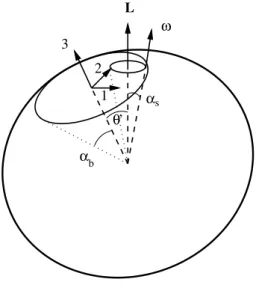
As a test for these equations we consider the case where c1=0, what means that the ellipsoids are not interacting and therefore free precession occurs. It is known (seee. g.Symon [15]) in this case that for each ellipsoid both polar principal symmetry axis (3-axis) and the rotation axis, which contains the angular velocity vectorω, have precession around the

con-served angular momentum vectorLforming the so called body cone and space cone, with semi-anglesαbandαs, respectively

(see Fig. 3). Notice that the 3-axis,ωandLare always in the

same plane. The constant angular velocity of such a precession around fixedLis

˙

φ′=βsinαb sinαs

ω3=

C

Acosθ′ω3 (24) with

’ 1 2 3

ω

α

α

b

s

L

θ

FIG. 3: Space and body cones generated by the Eulerian (free) preces-sion. The axes 1, 2 (equatorial principal axes) and 3 (polar principal axis) are fixed in the oblate ellipsoid and follow its motion. The angu-lar momentumLdefines a fixed direction in space while the angular velocityωgives the instantaneous rotation axis.

being the constant angle that gives the orientation of the prin-cipal 3-axis with respect to fixedL, and

tanαb= q

ω2 1+ω22 ω3

(26)

cosαs=

1+βcos2αb p

1+ (2+β)βcos2_α

b

(27)

β=C

A−1. (28)

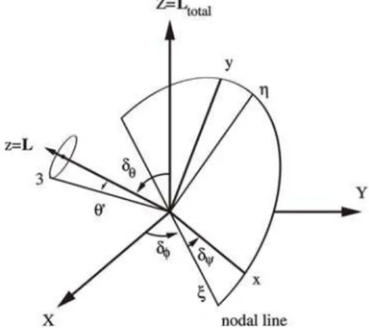
However, with two ellipsoids, we have a more general situa-tion where the fixed reference frame Z-axis is taken to be in the direction of the total angular momentumLt, which is

con-served if external torques are negligible, and not of the Earth angular momentumL. Therefore we define a reference frame xyz, such that z is in the direction ofL, oriented with respect to XYZ through the Euler anglesδθ,δφ,δψ(see Fig. 4). While the principal 3-axis has precession around z-axis with constant angular velocity ˙φ′ and angular amplitude θ′, the 3-axis has motion described in terms of the Euler anglesθ,φwith respect to the frame XYZ as

cosθ=sinθ′

sin(φ˙t+ε)sinδθsinδψ−cos(φ˙t+ε)sinδθcosδψ+cosθ′cosδθ (29) tanφ=−sinθ

′

B1sin(φ˙t+ε) +B2cos(φ˙t+ε)+cosθ′sinδθsinδφ sinθ′

B3sin(φ˙t+ε) +B4cos(φ˙t+ε)−cosθ′sinδθcosδφ

(30)

withεbeing an arbitrary phase and

B1 = cosδφcosδψ−cosδθsinδφsinδψ (31)

B2 = cosδφsinδψ+cosδθsinδφcosδψ (32)

B3 = sinδφcosδψ+cosδθcosδφsinδψ (33)

B4 = sinδφsinδψ−cosδθcosδφcosδψ. (34)

It can be verified using an algebraic calculation software thatθ andφgiven by equations (29) and (30) satisfy equations (20) and (21) withc1=0, what means that the latter equations de-scribe correctly the precessional motion around an axis ori-ented arbitrarily in space.

Before proceeding to the solution of equations (20)-(23) let us consider the elasticity of the Earth. This was first taken into account by Love [1] and Larmor [2] because the predicted free precession period was of 305 days while the observed value was of around 435 days. The correction due to Love introduces products of inertiaC13 andC23 in Euler equations (8)-(9) for the Earth (see Kaula [16]) which become

Aω˙1+ (C−A)ω2ω3−C23ω23+C˙13ω3=τ1 (35)

Aω˙2−(C−A)ω1ω3+C13ω23+C˙23ω3=τ2 (36)

with

C13 =

k2R5Eω3

3G ω1 (37)

C23 =

k2R5Eω3

3G ω2 (38)

whereREis the Earth mean radius andk2is the so called Love number. Therefore we obtain as a result

A+k2R

5

Eω23 3G

˙ ω1+

C−A−k2R 5

Eω23 3G

ω2ω3=τ1(39)

A+k2R

5

Eω23 3G

˙ ω2−

C−A−k2R 5

Eω23 3G

ω1ω3=τ2(40).

By comparing this with equations (8)-(9) we see that the over-all effect upon the last ones by the introduction of the elasticity of the Earth is to promote the transformation

A→A+k2R

5

Eω23

3G . (41)

The Love numberk2is left as one of the free parameters of this model.

FIG. 4: Free precession around an arbitrary axis z. The xyz-frame is oriented with respect to the XYZ-frame, which is fixed in space, through the Euler anglesδθ,δφ,δψ.

day/1000 = 86.4 s; changing this limit to 1 solar day/10000 did not cause meaningful modifications in the results. We have 11 free parameters, i. e., the Love numberk2, the momenta of inertiaA∗,C∗of the internal ellipsoid, and the following that establish the initial conditions: the componentsω∗

1∗,ω∗₂∗,ω∗₃∗ (recall that ω∗

3∗ is constant) of the angular velocityω∗in the principal axes 1∗2∗3∗of the internal ellipsoid, the Euler angles θ12=α,φ12,ψ12that give the spatial orientation of the 1∗2∗3∗ frame with respect to the 123 frame, and the angular velocities

˙

φand ˙φ∗_{. On the other hand, from equations (14) and (15) we} have

˙ θ=±

q

ω2

1+ω22−φ˙2sin2θ (42)

from which we can determine the initial value of ˙θunless by its sign. In an analogous way we have

˙ θ∗=±

q

ω∗2

1∗+ω∗₂2∗−φ˙∗2sin2θ∗. (43) From equations (42)-(43) we can also find bounds for the ini-tial guesses of ˙φand ˙φ∗

−

q

ω2 1+ω22 |sinθ| ≤φ˙≤

q

ω2 1+ω22

|sinθ| (44)

−

q

ω∗2 1∗+ω∗₂2∗

|sinθ∗_| ≤φ˙ ∗_≤

q

ω∗2 1∗+ω∗₂2∗

|sinθ∗_| . (45)

Besides, from energy conservation of the Earth-ellipsoid sys-tem, we have the following relation to be satisfied by the initial guesses ofω∗₁∗andω∗₂∗

ω∗12∗+ω∗₂2∗ ≥ c1

A[cos(2α)−1]− A A∗ ω

2 1+ω22

−2ω3

A∗ ×

×(C13ω1+C23ω2) (46)

whereαis the initial guess for the angle between the axes 3 and 3∗, andω1andω2are the initial components of the Earth angular velocityωin the axes 1 and 2, respectively.

H¨opfner [11, 12] has managed to filter the Chandler wobble (CW) and the annual wobble (AW) as major components from the data related to the Earth polar motion of its rotation axis around the polar principal axis. These data have being accu-mulated for more than 100 years and a compilation of them is published periodically by Gross [17] from NASA-JPL. We use a relation between the polar motion, described as the two an-glesPMX[ andPMY[, and the orientation of the Earth rotation axis, described by the anglesθωandφω(see Fig. 5). As usual, the 1-axis is towards the Greenwich meridian and the 2-axis is towards the 90◦E meridian. The anglesθωandφωcan be calculated from

ω

1

2

3

PMX

PMY

φ

ω

ω

θ

FIG. 5: Definition of the anglesPMX[ andPMY[ which describe the Chandler wobble motion. The origin of the 123-frame is at the Earth center. Axes 1 and 2 are towards the Greenwich meridian and 90◦E meridian, respectively. The 3-axis is the polar principal axis. The angular velocityωis also shown as well as its spherical coordinates

θωandφω.

tanθω=±

q

tan2_PMX[_+tan2_PMY[ ₍₄₇₎ tanφω=

tanPMY[

tanPMX[. (48)

Therefore by knowingPMX[andPMY[at the start of a Chandler wobble, taken from H¨opfner [11] calculations, and by know-ing the value of the length-of-day (LOD) at that moment, taken from Gross [17] data, we can calculate the initial values ofω1 andω2, which are necessary in equations (42), (44) and (46), and the value ofω3, which is considered as constant during the motion. Furthermore, we can calculate then the initial compo-nents of the Earth angular momentumLin the direction of the axes 123 as

L1 = Aω1+C13ω3 (49)

L2 = Aω2+C23ω3 (50)

the axes 1*2*3* by

L₁∗∗ = A∗ω∗₁∗ (52) L₂∗∗ = A∗ω∗₂∗ (53) L₃∗∗ = C∗ω∗₃∗. (54)

With these quantities available we can calculate the compo-nents of the total angular momentumLtin the axes 123

Lt1=L1+L∗1=L1+L∗1∗(cosφ12cosψ12−cosαsinφ12sinψ12)

−L∗₂∗(cosφ12sinψ12+cosαsinφ12cosψ12) +L∗3∗sinαsinφ12 (55)

Lt2=L2+L∗2=L2+L1∗∗(sinφ12cosψ12+cosαcosφ12sinψ12)

+L∗₂∗(−sinφ12sinψ12+cosαcosφ12cosψ12)−L∗3∗sinαcosφ12 (56)

Lt3=L3+L3∗=L3+L∗1∗sinαsinψ12+L∗2∗sinαcosψ12+L∗3∗cosα. (57)

X

Y

L

s t

=Z

L

L

*

u

_u

_*

3 3

θ

θ

*

φ

φ

*

s

FIG. 6: Definition of the frame XYZ fixed in space which is con-venient to describe both interacting ellipsoids motion. The Z-axis coincides with the direction of the total angular momentumLt. The XZ-plane is the same plane formed by theL(Earth) andL∗ (ellip-soid) angular momenta. The unit vectorsu3andu∗3, which are in the

direction of the polar principal axes 3 and 3*, are also shown as well as their spherical coordinatesθ,φs,θ∗,φ∗s.

Here, α=θ12,φ12 andψ12 are the initial guesses for the Euler angles that describe the 1∗2∗3∗reference frame with re-spect to the 123 frame. Since we define the Z-axis of the fixed reference frame in the same direction ofLt(see Fig. 6), the

ini-tial value of the Euler angleθ, that is necessary for the solution of equations (20)-(23), is obtained from

cosθ=Lt·u3 Lt

=_q Lt3 L2

t1+Lt22+Lt23

(58)

whereu3is a unit vector in the direction of the 3-axis. In order to calculate the initial value ofφwe construct the Y-axis as

orthogonal to theL∗L-plane (Fig. 6), taking the initial values of such vectors, and the X-axis orthogonal to the YZ-plane, as

FIG. 7: Calculated (line) and predicted (dots) Chandler wobble pro-grade (counter-clockwise) motion in the interval 44330-44755 (in modified Julian date - MJD) or 01/APR/1980-31/MAY/1981. The asterisk shows the position of the motion start point. PMX[ andPMY[

are given in milli-arcsec (mas).

usual. Then

cosφ=− u3Y

u3XY

=Lt2L1−Lt1L2

|L×Lt|sinθ

(59)

whereu3Y andu3XY are the projections ofu3in the Y-axis and in the XY-plane, respectively. In order to determine φ com-pletely we have also to express

sinφ= u3X u3XY

=Lt2(Lt2L3−Lt3L2)−Lt1(Lt3L1−Lt1L3) Lt|L×Lt|sinθ

.

(60) In an analogous way we have the projections ofLt in the axes

FIG. 8: Same as in Fig. 7, for the interval 44970-45403 (MJD) or 01/JAN/1982-10/MAR/1983.

Lt1∗ =L∗1∗+L1∗=L∗1∗+L1(cosφ12cosψ12−cosαsinφ12sinψ12)

+L2(sinφ12cosψ12+cosαcosφ12sinψ12) +L3sinαsinψ12 (61)

Lt2∗ =L∗₂∗+L2∗=L∗₂∗−L1(cosφ12sinψ12+cosαsinφ12cosψ12)

+L2(−sinφ12sinψ12+cosαcosφ12cosψ12) +L3sinαcosψ12 (62)

Lt3∗ =L∗₃∗+L3∗=L∗₃∗+L1sinαsinφ12−L2sinαcosφ12+L3cosα. (63)

FIG. 9: Same as in Fig. 7, for the interval 50170-50604 (MJD) or 28/MAR/1996-05/JUN/1997.

and the initial values for the Euler anglesθ∗ andφ∗ are ob-tained from

cosθ∗=Lt·u ∗

3

Lt

=q Lt3∗

L2_t1∗+L_t2₂∗+L2_t3∗

(64)

cosφ∗=−u

∗

3Y

u∗_3XY =

Lt1∗L∗₂∗−Lt2∗L∗₁∗

|L∗_×L

t|sinθ∗

(65)

sinφ∗= u∗_3X u∗_3XY =

Lt2∗(L_t3∗L∗₂∗−Lt2∗L∗₃∗)−Lt1∗(L_t1∗L∗₃∗−Lt3∗L∗₁∗) Lt|L∗×Lt|sinθ∗

.

(66)

While integrating equations (20)-(23) we can calculate the CW motion through (see Fig. 5)

tanPMX[=ω1 ω3

(67)

tanPMY[=ω2 ω3

(68)

FIG. 10: Relation between CW period (in days) and average ampli-tude (in mas). Circles represent results due to H¨opfner [11] while triangles show our results. The full line fits the last points. As a refer-ence, dashed and dotted lines represent fits for the epochs 1912-1928 and 1936-1948 respectively.

3. RESULTS AND DISCUSSION

With the aim of getting 10 unknown parameters of our model (all but k2) we find that it is enough to establish the following conditions: 1) reproduce the Chandler component of the Earth rotation axis position predicted by H¨opfner [11] at the start of a wobble; 2) minimize the length of the prograde (counter-clockwise) trajectory followed during that wobble motion. The second condition is necessary in order to avoid in-trusive nutations that might emerge accompanying the preces-sional motion. This means that we minimize, for a given initial guess ofk2, the sum of: a) the squared distance from the model calculed Earth rotation axis position(PMX[,PMY)[ at the start of the wobble and the one predicted by H¨opfner; b) the wob-ble trajectory length in the plane(PMX[,PMY)[ obtained by nu-merical integration. For this minimization process we used the

POWELLroutine from the Numerical Recipes package (Presset al. [18]). However the generalized simulated annealing (GSA) code (Mundim and Tsallis [19], Dall’Igna Junioret al. [20]) has proved to be very effective in a first step run in order to prevent getting stuck in local minima. The 11th parameter,k2, is then found by reproducing the Chandler component of the Earth rotation axis position at the end of the wobble, with ref-erence to H¨opfner’s prediction, so thatk2is responsible for the adjustment of a particular wobble period. We show in Figs. 7-9 some of our results for the CW in three different epochs, in comparison with the results due to H¨opfner [11], which are represented by dots. The first one, for whichω∗₃∗ is negative, has the typical quality of providing reasonable reproduction of the motion. The next Figures show the two exceptions to this rule, which tend to present almost circular trajectories instead of, in those epochs, the slightly elliptical ones due to H¨opfner. This may be caused by the above mentioned criteria – mainly condition 2) – adopted in the fit process. We also show in Table I the corresponding values for the 11 parameters (with respective numerical uncertainties shown in Table II), while in Table III we have the initial values of ˙θand ˙θ∗_calculated from equations (42) and (43) with appropriate signs and the corresponding values of the torque strengthc1. As expected – see comments after equation (7) – αturns out to be close

to 90◦. On the other hand, parametersω∗₃∗ (the main angu-lar velocity component of the ellipsoid),A∗,C∗andk2present oscillations when examining the respective columns in the Ta-ble I, being more noticeaTa-ble for the 44330-44755 interval. For k2, since it is connected to the period and that particular wob-ble has a short one – see Tawob-ble IV for a comparison between the presently calculated periods and the ones due to H¨opfner which they shall reproduce – this is not surprising although un-desirable. H¨opfner [11, 12], like other authors (seee. g.Liuet al.[21], Wang [22]), found variable CW periods but this is not a clearly solved question since some investigators have another opinion (seee. g. Vicente and Wilson [23], Jochmann [24], Liao and Zhou [25], Guoet al. [26]). For the sake of com-parison, values ofk2obtained by some other authors are 0.284 (Kaula [16]), 0.30088 (model 1066A of Gilbert and Dziewon-ski [27]) which are not far from what we got with the exception of the 44330-44755 case.

By comparing the values of C∗ with momenta of inertia of natural satellites present in the solar system we find that they range from about Miranda’s (Uranus) to Charon’s (Pluto). Since we are able only to calculate the DM ellipsoid prin-cipal momenta of inertia, which are related to the ellipsoid massM∗and their equatorial and polar radiia∗andc∗through A∗=M∗(a∗2_+c∗2_{)/5 andC}∗_=2M∗_a∗2_{/5, we cannot} estab-lish the ellipsoid mass uniquely, and in consequence, the frac-tion of DM present in the Earth is not predicted. Notice that, for an oblate ellipsoid, we havec∗≤a∗and, therefore, the re-lationC∗/2≤A∗≤C∗holds and it was required to be satisfied in our numerical procedure. Just to have an idea of the order of magnitude ofM∗, let us suppose thata∗≈2350 km,i. e., the ellipsoid has the average radius of the outer core of the Earth. From the values ofC∗in Table I, this implies that the fraction of DM present in the Earth would lie in the range 6×10−7 to 9×10−5. We emphasize that, according to the model, the Earth motion and its gravitational interaction with other bodies have already incorporated the presence of DM through what has been known effectively as “Earth mass”, so that the out-come of its presence might be more easily observed through the Earth wobble.

Following the hypothesis of changing CW periods we present in Fig. 10 the correlation between period and aver-age amplitude. We show H¨opfner’s results [11] and ours. The last ones are fitted by the full line, which has the form: pe-riod (in days) = 440–3101.47×exp[–0.0347946×amplitude (in mas)]. As a reference we also present the fits due to Liu et al [21] related to the epochs 1912-1928 and 1936-1948. The correlation clearly varies with time.

One might argue that the parameter fluctuations in Table I indicate that this model is not sound. However those fluctua-tions may be caused by the model simplistic – although con-venient at this stage – approach that we are considering the DM ellipsoid the only source responsible for the complexity of Chandler wobble, what obviously is not true. Therefore, the predictedA∗ andC∗dark matter ellipsoid parameters should be considered only as upper limit values.

TABLE I: Results for the 11 unknown parameters in several epochs: initial values for the angular velocities ˙φand ˙φ∗_{(in rad/s), for the}

componentsω∗₁∗,ω∗₂∗,ω∗₃∗(in rad/s) of angular velocityω∗, for the Euler anglesα=θ₁₂,φ₁₂,ψ₁₂(in degrees); values of the internal ellipsoid

principal momenta of inertiaA∗,C∗(in kg·m2) and Love numberk2.

interval φ˙ φ˙∗ _ω1∗

∗ ω∗2∗ ω∗3∗ φ12 ψ12 α A∗ C∗ k2

44330-44755 1.386E–7 3.087E–20 9.907E–12 4.140E–10 –1.592E–4 358.849 353.219 90.001 6.334E+32 1.264E+33 0.2672 44970-45403 –2.704E–5 –9.685E–7 –9.789E–7 –2.088E–9 4.952E–4 173.698 337.477 89.911 2.399E+31 3.334E+31 0.2801 45700-46135 5.711E–5 –4.203E–6 –4.262E–6 –2.128E–9 6.853E–4 359.988 359.999 89.847 1.079E+31 1.125E+31 0.2835 46340-46773 –7.419E–5 1.823E–6 3.935E–6 –2.410E–9 1.089E–3 187.700 350.276 89.849 7.429E+30 7.772E+30 0.2815 46977-47410 7.205E–5 –4.490E–6 –4.542E–6 –2.128E–9 7.455E–4 359.988 359.999 89.857 1.168E+31 1.211E+31 0.2815 47640-48075 –3.769E–5 2.098E–6 3.572E–6 –2.410E–9 7.727E–4 109.191 353.481 89.832 7.280E+30 7.548E+30 0.2842 48260-48696 5.317E–6 –1.861E–7 –1.862E–7 –2.128E–9 3.338E–3 222.469 359.999 90.047 1.947E+31 2.125E+31 0.2861 48900-49336 –2.505E–5 –1.142E–6 –1.142E–6 –2.088E–9 5.632E–4 346.867 332.210 89.841 1.731E+31 1.903E+31 0.2869 49630-50066 4.133E–5 –6.759E–6 –6.759E–6 –2.128E–9 7.390E–4 359.988 359.999 89.873 9.482E+30 9.710E+30 0.2869 50170-50604 –3.317E–5 –6.301E–7 –6.301E–7 –2.088E–9 5.230E–4 247.397 333.076 89.877 8.287E+30 9.587E+30 0.2824

TABLE II: Numerical uncertainty estimates (in %) of the parameters shown in Table I.

interval

∆ ˙φ

˙ φ

∆ ˙φ∗ ˙ φ∗

∆ω∗

1∗ ω∗ 1∗

∆ω∗

2∗ ω∗ 2∗

∆ω∗

3∗ ω∗ 3∗ ∆φ12 φ12 ∆ψ12 ψ12 ∆α α

∆A∗

A∗

∆C∗

C∗ ∆k2 k2

44330-44755 0.10 4.6E–6 1.3E–7 2.3E–9 71 1.6E–3 1.6E–2 6.6E–4 1.1E–3 129 1.1E–4 44970-45403 1.8E–6 0.95 0.77 3.0E–5 2.5E–7 2.2 0.37 5.0E–2 4.1E–6 28 1.1E–3 45700-46135 9.6E–6 1.5 0.16 1.8E–6 1.6E–6 4.5E–8 1.9E–10 9.1E–6 4.3 1.8 1.2E–5 46340-46773 3.0E–4 0.44 0.11 3.7E–5 13 16 2.8E–2 3.1E–4 4.6 7.0 6.6E–5 46977-47410 1.2E–6 1.3 0.64 2.7E–5 6.2E–7 7.2E–8 <1E–13 7.9E–6 3.8 3.5 5.8E–5 47640-48075 3.6E–4 3.8 0.26 2.0E–5 1.6E–5 6.2 3.5E–2 7.4E–5 4.1 1.3 1.2E–4 48260-48696 3.3E–5 2.8E–2 1.7E–3 3.4E–5 38 26 7.7E–10 7.0E–6 14 22 4.9E–5 48900-49336 8.3E–5 1.1 1.9 5.0E-5 4.6 0.34 1.4 1.5E–5 9.9 13 1.6E–4 49630-50066 <1E–13 2.6 6.8E–2 2.6E–7 1.6E–3 7.9E–14 <1E–13 3.2E–9 2.7 0.38 2.5E–5 50170-50604 2.7E–5 2.3 1.0E–6 3.0E–6 <1E–13 1.1E–2 2.2E–2 2.7E–9 18 11 1.3E–4

dependent, gravitational field with two contributions, with re-spect to au1u2u3reference frame attached to the Earth. The first term is radial:

ar=

3G(C∗−A∗) 2r4

3 sin2θ(cosφsinωTt+sinφcosωTt)2−1

. (69)

Here,θis the co-latitude,φis the longitude andωT is the Earth

angular velocity. Of course,ωTtis defined except for a phase

that would establish the position of the ellipsoid rotation axis with respect to the Greenwich meridian (for instance, in the direction ofu1), at a given time. The second contribution is

aθ∗ =3G(C ∗_−A∗₎ 2r4 sin 2θ

∗_[(cosθ∗_sinφ∗_cosω

Tt−sinθ∗sinωTt)u1

−(cosθ∗sinφ∗sinωTt+sinθ∗cosωTt)u2+cosθ∗cosφ∗u3] (70)

where

sinθ∗=

q

cos2_θ+sin2_{θ(cosφcosω}

Tt−sinφsinωTt)2

(71) cosθ∗=sinθ(cosφsinωTt+sinφcosωTt))

(72)

sinφ∗=q sinθ(cosφcosωTt−sinφsinωTt)

cos2_θ+sin2_{θ(cosφcosω}

Tt−sinφsinωTt)2

(73)

cosφ∗=q cosθ

cos2_θ+sin2_{θ(cosφcosω}

Tt−sinφsinωTt)2

.

TABLE III: Calculated initial values of ˙θand ˙θ∗(in rad/s), with respective appropriate signs, and torque strengthc1(in N·m2).

interval θ˙ θ˙ c1

44330-44755 2.426E–11 4.141E–10 9.226E+23 44970-45403 –2.684E–11 1.419E–07 1.367E+22 45700-46135 –4.176E–11 7.080E–07 6.790E+20 46340-46773 3.218E–11 3.487E–06 5.006E+20 46977-47410 –2.231E–11 6.839E–07 6.349E+20 47640-48075 3.367E–11 2.891E–06 3.922E+20 48260-48696 –4.771E–12 –4.521E–09 2.607E+21 48900-49336 –9.816E–12 1.147E–08 2.517E+21 49630-50066 –5.563E–11 3.185E–10 3.331E+20 50170-50604 –4.110E–11 4.946E–10 1.900E+21

TABLE IV: CW periods resulting from the model in comparison with the values from H¨opfner [11] (in days).

interval calculated period H¨opfner’s period

44330-44755 424.578 424.76 44970-45403 432.454 432.45 45700-46135 434.677 434.68 46340-46773 433.366 433.37 46977-47410 433.331 433.33 47640-48075 435.123 435.12 48260-48696 436.414 436.41 48900-49336 436.943 436.93 49630-50066 436.924 436.92 50170-50604 433.920 433.92

Note that, in the Earth’s reference frame, the DM ellipsoid gives a complete turn in a day. Supposing the DM ellipsoid is smaller than the Earth core, this gravitational field certainly enforces viscous flow in the outer core, which is in a fluid state. As a first consequence, it can provide the necessary energy to the magneto-hydrodynamic motion in the outer core, which is closely related to the generation of the geomagnetic field. This could give a plausible explanation to one of the basic prob-lems of geophysics (see Stacey, ref. [13]), namely, what is the source of this energy. However the numerical solution of this motion through the Navier-Stokes and energy conservation

equations suffers lack of knowledge of the flowing material density dependence with respect to pressure and temperature. Secondly, it can generate heat in the core, that would contribute to decrease the shortfall of 0.7 TW to the energy necessary to maintain the adiabatic temperature gradient in the core, leaving more power to drive the geomagnetic field dynamo [13]. On the other hand, Macket al. [28] have concluded that DM is unlikely to contribute not only to Earth’s internal heat flow but also to hot-Jupiter exoplanets. However they studied the con-tribution of DM self-annihilation to heat generation, what is a different idea from ours. Conversely, Adler [9] has also studied the contribution of self-annihilating and non-self-annihilating DM accretion to the internal heat of the Earth, Jovian planets and hot-Jupiter exoplanets. His conclusion is that this process is plausible provided efficient DM capture is occurring. In our description, it is feasible to imagine DM ellipsoids also present is such bodies, generating heat by enforcing internal viscous flow, like in Earth. Therefore this model can mean much more than mere emulation of known suggested causes for CW but it also touches open questions like geomagnetic field dynamo and heat generation in the Earth’s outer core and in other plan-ets.

Rather than giving the final answer for the problem that has raised the attention of geophysicists and astronomers for sev-eral decades, we expect that this calculation may open room for a new and potentially important key component in CW which was completely unsuspected untill now, to be consid-ered in more sophisticated models. Future development will decide about the real significance of this approach that might have relevant consequences in our comprehension about dark matter. At least, it has been demonstrated that two interacting ellipsoids can have Chandler-like wobble.

ACKNOWLEDGMENTS

The author would like to thank Prof. Joachim H¨opfner (re-tired from GFZ-Potsdam) for enlightening correspondence and for providing unpublished results, Prof. Kleber C. Mundim, from Chemistry Institute-University of Brasilia, for allowing the use of his GSAcode, Prof. Nivaldo A. Lemos, from Uni-versidade Federal Fluminense, for correspondence in the early stages of this work, Prof. Marcos D. Maia, from Institute of Physics-University of Brasilia, for his interest and for pointing me some related literature, Prof. Marcus B. Lacerda Santos, also from Institute of Physics-University of Brasilia, for stim-ulating discussions, and MEC-SESu for tutorship (PET pro-gram). Finally, thanks are due to the Referee of this paper, for interesting remarks.

[1] A. E. H. Love, Proceedings of the Royal Society of LondonA 82, 73 (1909).

[2] J. Larmor, Proceedings of the Royal Society of LondonA 82, 89 (1909).

[3] M. L. Smith and F. A. Dahlen, Geophysical Journal of the Royal Astronomical Society64, 223 (1981).

[4] R. S. Gross, Geophysical Research Letters27, 2329 (2000).

[5] F. Seitz, J. Stuck and M. Thomas, Geophysical Journal Interna-tional157, 25 (2004).

[6] C. D. Froggatt and H. B. Nielsen, Physical Review Letters95, 231301 (2005).

[7] J.-M. Fr`ere, F.-S. Ling and G. Vertongen, Physical ReviewD 77, 083005 (2008).

Potter and J. Stadel, Nature 454, 735 (2008); arXiv:astro-ph/0805.1244.

[9] S. L. Adler, arXiv:astro-ph/0808.2823.

[10] S. Khalil and C. Mu˜noz, Contemporary Physics43, 51 (2002); arXiv:hep-ph/0110122.

[11] J. H¨opfner, Journal of Geodynamics36, 369 (2003). [12] J. H¨opfner, Surveys in Geophysics25, 1 (2004).

[13] F. D. Stacey,Physics of the Earth(Brookfield Press, Brisbane, 1992).

[14] A. M. Dziewonski and D. L. Anderson, Physics of the Earth and Planetary Interiors25, 297 (1981).

[15] K. R. Symon,Mechanics(Addison-Wesley, Reading, 1971). [16] W. M. Kaula,An Introduction to Planetary Physics(Wiley, New

York, 1968).

[17] R. S. Gross, Combinations of Earth orientation mea-surements: SPACE2004, COMB2004, and POLE2004, JPL-NASA publication 05-6 (Pasadena, California, 2005); ftp://euler.jpl.nasa.gov/keof/combinations/2004.

[18] W. H. Press, B. P. Flannery, S. A. Teukolsky and W. T. Vetter-ling,Numerical Recipes in Fortran 77(Cambridge University Press, Cambridge, 1999).

[19] K. C. Mundim and C. Tsallis, International Jour-nal of Quantum Chemistry 58, 373 (1996); preprint http://www.unb.br/iq/kleber/GSA/gsa-java/index.htm.

[20] A. Dall’Igna Junior, R. S. Silva , K. C. Mundim and L. E. Dard-enne, Genetics and Molecular Biology27, 616 (2004). [21] L. T. Liu, H. T. Hsu, B. X. Gao and B. Wu, Geophysical

Re-search Letters27, 3001 (2000).

[22] W. J. Wang, Geophysical Journal International158, 1 (2004). [23] R. O. Vicente and C. R. Wilson, Journal of Geophysical

Re-search102, 20439 (1997).

[24] H. Jochmann, Journal of Geodesy77, 454 (2003).

[25] D. C. Liao and Y. H. Zhou, Chinese Journal of Astronomy and Astrophysics4, 247 (2004).

[26] J. Y. Guo, H. Greiner-Mai, L. Ballani, H. Jochmann and C. K. Shum, Journal of Geodesy78, 654 (2005).

[27] F. Gilbert and A. M. Dziewonski, Philosophical Transactions of the Royal Society of LondonA 278, 187 (1975).