Online-SVR for short-term traffic flow prediction under typical and atypical
traffic conditions
Manoel Castro-Neto
a,1, Young-Seon Jeong
b,2, Myong-Kee Jeong
b,*, Lee D. Han
a,3 aDepartment of Civil and Environmental Engineering, University of Tennessee, Knoxville, TN 37996, USA bDepartment of Industrial and Systems Engineering, Rutgers University, Knoxville, Piscataway, NJ 08854, USA
a r t i c l e
i n f o
Keywords:
Short-term flow forecast
Intelligent transportation systems (ITS) Online support vector machine (OL-SVM) Online support vector regression (OL-SVR) Traffic volume prediction
a b s t r a c t
Most literature on short-term traffic flow forecasting focused mainly on normal, or non-incident, condi-tions and, hence, limited their applicability when traffic flow forecasting is most needed, i.e., incident and atypical conditions. Accurate prediction of short-term traffic flow under atypical conditions, such as vehicular crashes, inclement weather, work zone, and holidays, is crucial to effective and proactive traffic management systems in the context of intelligent transportation systems (ITS) and, more specifically, dynamic traffic assignment (DTA).
To this end, this paper presents an application of a supervised statistical learning technique called Online Support Vector machine for Regression, or OL-SVR, for the prediction of short-term freeway traffic flow under both typical and atypical conditions. The OL-SVR model is compared with three well-known prediction models including Gaussian maximum likelihood (GML), Holt exponential smoothing, and arti-ficial neural net models.
The resultant performance comparisons suggest that GML, which relies heavily on the recurring char-acteristics of day-to-day traffic, performs slightly better than other models under typical traffic condi-tions, as demonstrated by previous studies. Yet OL-SVR is the best performer under non-recurring atypical traffic conditions. It appears that for deployed ITS systems that gear toward timely response to real-world atypical and incident situations, OL-SVR may be a better tool than GML.
Ó2008 Elsevier Ltd. All rights reserved.
1. Introduction
1.1. Research problem
The use of inductive loops for vehicle detection predates Intel-ligent Transportation Systems (ITS) by decades. Since the 1990s the advent of ITS, particularly one of its key components advanced traffic management systems (ATMS), saw an extensive and system-atic deployment of various vehicular detection technologies on the Nation’s Interstate and other major arterials. These increasingly sophisticated and widely deployed sensors, once online, begin to generate voluminous real-time traffic data continuously; some have been at it for years. The intended use of these data is to em-power traffic engineers to monitor real-time traffic condition and,
subsequently, manage and improve the operational efficiency and safety of the Nation’s roadway system in a timely fashion.
To assess the traffic condition across all travel lanes at a partic-ular point along a highway, it is common, and usually necessary to instrument each lane with at least one detector. The detectors de-ployed at a single location are collectively known as a vehicle detec-tor station (VDS) and their data are often aggregated and reported together. These data typically include volume (vehicle counts) and occupancy (amount of time a detector is ‘‘hot”) for the report-ing time period, which is usually 30 s. Other traffic flow parameters such as average speed, vehicular density, and average travel time can be derived from these data with reasonable accuracy.
These data, and the traffic condition information they represent, are essential to many ITS applications including dynamic traffic assignment (DTA), which provides routing information to the motoring public using sophisticated optimization algorithms based on estimated origin–destination (OD) demand and locale-based traffic conditions.
It did not take long for researchers and practitioners to recog-nize that the benefits of ITS cannot be fully realized if traffic parameters are not ‘‘known” in advance or, in other words, fore-casted (Smith, Williams, & Oswald, 2002). Without a ‘‘look-ahead”
0957-4174/$ - see front matterÓ2008 Elsevier Ltd. All rights reserved. doi:10.1016/j.eswa.2008.07.069
*Corresponding author. Tel./fax: +1 732 445 4858.
E-mail addresses:mcastron@utk.edu (M. Castro-Neto),yjeong@utk.edu(Y.-S. Jeong),mjeong@utk.edu(M.-K. Jeong),lhan@utk.edu(L.D. Han).
1
Tel.: +1 865 974 7733. 2
Tel.: +1 865 974 7650. 3 Tel.: +1 865 974 7707.
Contents lists available atScienceDirect
Expert Systems with Applications
mechanism, ATMS can only operate in a reactive manner. On the other hand, if traffic conditions can be accurately forecasted, ATMS can be more proactive and, hence, more effective in identifying and addressing problems in a timely fashion. Not only such a proactive system can mitigate and minimize the adverse effects of traffic problems, but it can also have the potential of avoiding the onset of such traffic problems in the first place. This is a major incentive of many short-term traffic flow prediction studies in the past.
The vast majority, if not all, of the published studies have pre-dominantly dealt with the prediction of short-term traffic flow un-der ‘‘typical” traffic operational conditions. In other words, the studies have focused mainly on normal, or non-incident, conditions. While it is understandable for researchers to confront an intellec-tual challenge with its simplest form, by avoiding ‘‘atypical” traffic conditions, the prediction problem becomes relatively simplistic and arguably unnecessary. To this end, this study adds the consid-eration of atypical traffic conditions so the resultant prediction model is more realistic and useful in for real-world ITS applications.
1.2. Objective of study
Given both the importance of predicting short-term traffic flow under unusual traffic situations and the lack of research addressing this problem, the main objective of this study is to perform short-term freeway traffic flow predictions when traffic is under abnor-mal conditions by using online support vector machine for regres-sion (OL-SVR). The prediction performance of OL-SVR was compared to those of other three commonly used models: a model proposed by Lin based on the Gaussian maximum likelihood esti-mation method (GML) (Lin,2001), neural network (NNet), and Holt exponential smoothing (ES).
Event though this research focuses on traffic under unusual conditions, the performance of the four prediction models were also evaluated for traffic under its regular regime.
2. Literature review – theoretical background
2.1. Short-term traffic flow prediction: previous efforts
The advance of computing and the significant increase of real-time ITS data availability have allowed researchers to develop and apply new methodologies to forecast traffic flow in real-time. Several papers have been published over the last three decades on this subject.
Since the 1970s, univariate time series models have been widely used for short-term traffic flow prediction, especially Box–Jenkins autoregressive integrated moving average (ARIMA) models (Der Voort, Dougherty, & Watson, 1996; Hamed, Al-Masaeid, & Said, 1995; Hamed & Cook, 1979; Lee & Fambro, 1999; Levin & Tsao, 1980; Smith & Demetsky, 1997; Williams, Prya, & Brown, 1998). Nowadays, ARIMA and exponential smoothing (ES) models such as Holt–Winters have been used for comparison purposes whenever a new forecasting model for short-term traffic is proposed (Park, Messer, & Urbanik, 1998).
Over the last decade, NNet models have been extensively used in the field of transportation engineering. Not only flow, but also other traffic parameters including speed (Ishak & Alecsandru, 2004; Ishak, Kotha, & Alecsandru, 2003; Xiao, Sun, Ran, & Oh, 2003; Xiao, Sun, Ran, & Oh, 2004), travel time (Dia, 2001; Vanajak-shi & Rilett, 2004), and occupancy (Zhang, 2000), have been pre-dicted in real-time by NNet models. Regarding short-term prediction of traffic flow only, a dynamic wavelet NNet model was used to predict hourly traffic flow, including time of the day and day of the week as variables in the model (Jiang & Adeli, 2000). Reference Lingras, Sharma, Osborne, and Kaylar (2000)
applied time-delay NNet and Park (2002) employed a hybrid neu-ro-fuzzy methodology, where initially fuzzy C-means (FCM) was used to classify traffic patterns into clusters, and then radial basis function (RBF) NNet was used to forecast traffic within clusters. In Zheng, Lee, and Shi (2006) a Bayesian combination of back-propa-gation NNet and RBF NNet was used to make short-term flow fore-casts. Many other relevant papers have used NNet for short-term traffic flow forecasting, including Smith and Demetsky (1995), Smith and Demetsky (1997), Chang (1999), Chen and Grant-Muller (2001), Dougherty and Cobett (1997), Kirby, Watson, and Dougher-ty (1997), Kwon and Stephanedes (1994), Vlahogianni, Karlaftis, and Golias (2005), Yasdi (1999), Yun, Namkoong, Rho, Shin, and Choi (1988) and Zhong, Sharma, and Lingras (2005). In many of the most recent papers, NNet has been used as a benchmarking method to be compared with new proposed techniques.
Several other techniques have been applied to predict real-time traffic flow, including multivariate state space time series (Stathopoulos & Karlaftis, 2003), multivariate non-parametric regression (Clark, 2003; Smith & Demetsky, 1996), nearest neigh-bor non-parametric regression (Davis & Nihan, 1991; Smith et al., 2002), dynamic generalized linear models (Lan & Miaou, 1999), and Kalman filtering models (Okutani & Stephanedes, 1984).
Lin (2001)proposed a forecasting model based on the Gaussian maximum likelihood (GML) estimation method to perform one-step ahead forecasts using 5-min traffic flow data. This methodol-ogy used both current and historical data traffic in an integrated way. Two years later, another study was published comparing Lin’s GML approach with three other models for hourly flow prediction, namely non-parametric regression (NPR), ARIMA, and NNet (Tang, Lam, & Ng, 2003). Again, the GML-based model presented the best forecasting performance. In another case study, the performance of the Lin’s GML-based model was compared again with those of NPR, ARIMA, and NNet for 87 VDS’s in Hong Kong (Lam, Tang, Chan, & Tam, 2006). The authors concluded that the GML method provided the best performance. However, they hypothesize that this model would not work when the traffic pattern is disturbed. Since the GML approach performed well in those three studies, it was one of the four prediction models assessed in this paper.
Recently, ordinary support vector regression (SVR) has been successfully used to predict traffic parameters such as hourly flow (Ding, Zhao, & Jiad, 2002), and travel time (Wu, Ho, & Lee, 2004). This approach can avoid overfitting which is likely to occur with NNet models. However, in most ITS applications, where new traffic data become available in every couple of minutes or seconds, the traditional SVR method is not a practical option because it requires complete model training whenever a new data point is added. Therefore, the online version of SVR, known as OL-SVR, is proposed in this research for short-term traffic flow forecasting. To the best of the authors of this paper’s knowledge, at the time of this writing no application of OL-SVR has ever been presented to predict traffic parameters.
2.2. Online-SVR
A detailed description of OL-SVR algorithm is given in Ma, James, and Simon (2003). Given a set of data points ðx1;y1Þ;
ðx2;y2Þ;. . .;ðxm;ymÞ for online prediction, where xi2X#Rn;yi2
Y#Rn and m is the total number of training samples, a linear regression function can be stated as
fðxÞ ¼wT
UðxiÞ þb ð1Þ
in a feature spaceF; wherewis a vector inFandU(xi) maps the
minimize 1 2w
TwþCP
m
i¼1 ðnþi þn
iÞ
subject to
yiwTUðxiÞ b6eþn þ i wT
U
ðxiÞ þbyi6eþn i nþi;n
i P0;
8 > < > : ð2Þ
where
e
(P0) is the maximum deviation allowed during the train-ing andC(>0) is the associated penalty for excess deviation during the training. The slack variables,nþi andni;correspond to the size of
this excess deviation for positive and negative deviations respec-tively. The first term in(2),wTw, is the regularized term, thus it con-trols the function capacity; the second termðPm
i¼1ðnþi þniÞÞis the
empirical error measured by the
e
– insensitive loss function. There-fore, the KKT conditions for OL-SVR can be rewritten asoLD
o
a
i¼X
l
j¼1
Qijð
a
ja
jÞ þeyiþfdiþui¼0;oLD
o
a
i¼ X
l
j¼1
Qijð
a
ja
jÞ þeþyifdi þu i ¼0;dðÞi P0;dðÞi
a
ðÞi ¼0;uðÞ i P0;u
ðÞ i ð
a
ðÞ
i CÞ ¼0; ð3Þ
wherefin(3)is equal tobin(1)at optimality (Chang & Lin, 2002). According to the KKT conditions, in(3), at most one of
a
ianda
iwillbe nonzero and both are nonnegative. Therefore, a coefficient differ-encehiwas defined as
hi¼
a
ia
i; ð4Þwherehidetermines both
a
ianda
i. In addition, a margin functionh(xi) for theith samplexiis defined as
hðxiÞ fðxiÞ yi¼
X
l
j¼1
Qijhjyiþb: ð5Þ
Therefore, combining(3)–(5)leads to the following five conditions:
hðxiÞPe; hi¼ C
hðxiÞ ¼e; C<hi<0
e6hðxiÞ6e; hi¼0 ð6Þ
hðxiÞ ¼ e; 0<hi<C
hðxiÞ6e; hi¼C:
In the OL-SVR approach, the regression parameters must be incrementally increased or decreased each time a new sample is added. To achieve this, the five conditions in(6)can be represented by three subsets into which the samples in a training setTcan be classified:
TheESet : Error support vectors :E¼ fijjhij ¼Cg ð7Þ
TheSSet : Margin support vectors :S¼ fij0<jhij<Cg ð8Þ
TheRSet : Remaining samples :R¼ fijhi¼0g: ð9Þ
The initialization of the algorithm uses two samples to generate the SVR coefficients and uses these coefficients to train the remain-ing part of the trainremain-ing set usremain-ing three samples at a time. Once the training is completed, both the online testing and predictor updat-ing follows.
2.3. Models for comparison
2.3.1. Artificial neural networks
NNet are nonlinear devices that are trained in a supervised manner to adjust their weights to minimize an objective function (Dreyfus, 2005). In particular, multi-layer perceptron (MLP)
algo-rithm, which has the special nodes named hidden nodes, was in-vented to solve nonlinearity problems that cannot be solved with a single layer network. MLP algorithms have been extensively ap-plied for forecasting traffic parameters such as travel speed, travel time and flow (Chen, Grant-Muller, Mussone, & Montgomery, 2001; Florio & Mussone, 1996; Tang et al., 2003; Vanajakshi & R. Rilett, 2004). The training of the network is based on back-prop-agation learning algorithm, where the error calculated at the out-put of the network is propagated through the layers of neurons to update the weights.
2.3.2. Holt’s exponential smoothing
Exponential smoothing (ES) techniques are relatively simple and effective methods for time series forecast for short-term hori-zons (De Lurgio, 1998). Holt ES has been widely used to both smooth and forecast time series data where trend, but not season-ality, is present. Since its forecast pattern is linear, Holt ES tends to not perform well for multiple-step ahead forecasts Holt’s tech-nique is implemented by using the following formulation:
St¼
a
Ytþ ð1a
ÞðSt1þbt1Þbt¼bðStSt1Þ þ ð1bÞbt1
Ftþm¼Stþbtm;
ð10Þ
where
a
andbare the smoothing constants,Stis the smoothed valueat the end of periodt,btis the smoothed trend in periodt, andmis
the forecasting horizon. The two smoothing constants (
a
andb) can be either subjectively chosen by the user or objectively optimized based on a criterion such as MSE or MAPE. Smoothing constants close to 1 put more weights on the most recent observations, while smoothing constants close to 0 allow distant past observations to have a larger influence on prediction. Also, to initialize the smooth-ing process, initial values ofS1 andb1 are needed, which can beaccomplished by backcasting. For those familiar with ARIMA mod-els, Holt’s ES is equivalent to ARIMA (0, 2, 2).
2.3.3. Gaussian maximum likelihood (GML) approach
Lin’s GML-based model makes use of both historical and real-time information in an integrated way by using two key variables: flow and flow increment (Lin, 2001). Let Xi;d, i= 0, 1, 2,. . . and
d= 0, 1, 2,. . . be consecutive observations of the traffic flow obtained at time i of day d. Let Yi;d¼Xi;dXi1;d be the flow
increment. Assuming that these two variables are normally distrib-uted, an estimate for the flow in the next periodiwas derived by maximizing the product of the two probability functions of Xi;d
andYi;d, resulting in the simple model:
^xi;d¼
r
2x;ið
l
y;iþxi1;dÞ þr
2y;il
x;ir
2 x;iþr
2 y;i
; i¼1;2;3;. . . ð11Þ
where
l
x,iandr
2x;iare the mean and variance ofXi, respectively, andl
y,iandr
2y;i are the mean and variance of Yi, respectively. Thesemeans and variances are estimated from the empirical data. Notice in(11)that flow at timeiis predicted based on the ob-served flow at timei1, on the historical mean and variance of the flows at time i, and on the historical mean and variance of the flow increments related to timesi andi1. More details of Lin’s GML-based model can be found inLin (2001).
3. Data description
purposes. Besides loop-detector data, the PeMS also provides traf-fic incident data collected by the California Highway Patrol (CHP). CHP provides incident data in real-time with incident characteris-tics, including type of incident, starting time, location, and subse-quent details about the incident (California Highway Patrol (CHP), 2006).
Other ITS studies involving prediction of short-term traffic parameters have been done using the PeMS database, including Yang, Yin, Liu, and Ran (2004). Detailed information about the PeMScan be found in the system’s website.
3.1. Data resolution (aggregation level)
The resolution (aggregation level) of the data plays an impor-tant role in short-term traffic forecasting (Dougherty & Cobett, 1997). Loop-detector traffic data with high-resolution (less than 1 min) tend to be very noisy, which decreases the forecasting capa-bility of the prediction models, whereas data with low resolution obviously provide less information about the traffic. Abdulhai, Porwal, and Recker (2002) showed the effect of the aggregation level of the data on the performance of forecasting models for short-term traffic flow and found that, the higher the resolution of the data, the higher the prediction error. They also concluded that the resolution of the data should be equal to that of the data to be predicted. For instance, if the objective is to forecast traffic in 5-min periods into the future, then probably the best data reso-lution to be used is 5-min. Therefore, aggregation of high-resolu-tion raw detector data into lower resoluhigh-resolu-tion levels is a common practice in short-term traffic forecasting studies. For instance, raw loop-detector data have been aggregated into 15-min (Chen & Grant-Muller, 2001), 10-min (Clark, 2003), and 5-min (Chen, Dougherty,& Kirby, 2001; Park, 2002), periods before the forecast-ing models were applied. More detailed research on aggregation level of ITS data can be found inQiao, Yu, and Wang (2003) and Qiao, Yu, and Wang (2004).
Based on the literature review, on the characteristics of both the data and the prediction models, and on the research purposes, 5-min data were used on this research. This was the same aggrega-tion level used in the study that introduced GML-based model for short-term traffic prediction (Lin, 2001).
3.2. Scenarios of study
The prediction accuracy of the models was assessed with traffic under two scenarios, which are described as follows:
3.2.1. Scenario 1 – typical traffic conditions
In this scenario, no special occurrences that may significantly change the traffic pattern, such as vehicle collisions, were present. For each of the 7 randomly selected freeway locations, 16 days of 5-min traffic flow data from 5:00 am to 10:00 am were collected, summing up to a total of 107,520 (960 observations/VDS/day7 VDSs16 days) observations. Only data from Tuesdays, Wednes-days and ThursWednes-days were included because traffic behavior on these days is considered ordinary. The first 15 days of data were available for model training, and the 16th day was used for model testing.Table 1shows some characteristics of the 7 stations used in scenario 1.
3.2.2. Scenario 2 – atypical traffic conditions
The only difference between scenario 1 and scenario 2 is that in this scenario, the testing day (16th day) either was a special day of traffic (holiday), or had an unexpected event (traffic incident) occurring near the VDSs analyzed. In all other fifteen days available for model training, the traffic on all seven VDSs presented their typical pattern, where no special day or event occurred.Table 2 de-scribes some the characteristics of the seven stations used in sce-nario 2.
Regarding the quality of the data used in this study, the PeMS provides the percentage of the data that were actually observed, as opposed to estimated (imputed). In each VDS selected in this study, 100% of the testing data and more than 90% of the training data were actually observed.
4. Forecasting approach
4.1. Implementation of OL-SVR
For the implementations of OL-SVR, we used a typical online time series prediction scenario and used a prediction horizon of one time step. The procedure used is that after considering given a time seriesxðtÞ;t¼1;2;. . . and prediction originO, time from which the prediction is generated, we constructed a set of training samples,AO;B, from the segment of time seriesfxðtÞ; t¼1;. . .;Og as AO;B¼ fXðtÞ;yðtÞ; t¼B;. . .;01g, where XðtÞ ¼ ½xðtÞ;. . .;xðt
Bþ1ÞT,yðtÞ ¼xðtþ1Þ, andBis the embedding dimension of the training setAO;B. We trained the predictorPðAO;B;XÞfrom the
train-ing set AO;B. Then, we predicted xðOþ1Þ using ^xðOþ1Þ ¼
PðAO;B;XðOÞÞ. Whenx(O+ 1) becomes available, we update the
pre-diction origin; that is,O=O+ 1 and repeat the procedure. As the origin increases, the training set keeps growing and this can be-come very expensive. However, online prediction take advantage of the fact that the training set is augmented one sample at a time and continues to update and improve the model as more data
be-Table 1
VDSs characteristics in scenario 1: traffic under typical conditions
VDS Freeway County Testing day Event Testing time (am)
1 I-5 N San Diego August/26/2006 None 5:00–10:00 2 I-5 N San Diego August/26/2006 None 5:00–10:00 3 SR-101 N San Francisco August/26/2006 None 5:00–10:00 4 I-5 S Lathrop August/26/2006 None 5:00–10:00 5 I-10 W Los Angeles August/26/2006 None 5:00–10:00 6 I-5 S San Diego August/26/2006 None 5:00–10:00 7 I-880 S Alameda August/26/2006 None 5:00–10:00
Table 2
VDS characteristics in scenario 2: traffic under atypical conditions
VDS Freeway County Testing day Event Event time (am)
1 I-5 N San Diego July/04/2006 Holiday 5:00–10:00
2 I-580 W Alameda August/29/2006 Traffic collision 6:47–7:42
3 I-880 S Oakland August/24/2006 Traffic collision 7:49–8:47
4 SR-170 S Los Angeles August/24/2006 Traffic collision 9:15–10:40
5 I-5 S San Joaquin July/04/2006 Holiday 5:00–10:00
6 SR-57 N Orange August/31/2006 Traffic collision 7:36–9:02
come available. For OL-SVR implementations, we use RBF kernel defined as expðpjxixjj2Þ.
Stating in simpler words, the OL-SVR training procedure was done in the following way. In each of the 15 training days, the first 10 data points (flows from 5:05 am to 5:50 am) were used as input, with the 11th data point (flow at 5:55 am) being the target. Then, the 10-point input window ‘‘walks”, incorporating the 11th data point, which results on a new 10-point input window (flows from 5:10 am to 5:55 am), having then the 12th data point (flow at 6:00 am) as the target. The process continues until the last obser-vation (flow at 10:00 am) becomes the target. After the model parameters are calibrated, the model is tested on the 16th day of data, predicting traffic flows from 6:20 am to 10:00 am, resulting in 45 one-step ahead forecasts in each VDS, in each scenario.
4.2. Implementation of (NNet)
In this paper, the architecture of MLP was composed as follows: ten neurons in the input layer, single hidden layer with 4 neurons and 1 output neuron. The input neurons include the fxðtÞ;t¼1;2;. . .gwhile the output neuron isxðtþ1Þ, witht repre-senting the current time.. The input neurons include the fxðkÞ;k¼t9;. . .;tg while the output neuron is x(t+ 1), witht
representing the current time. Tangent sigmoid function and linear transfer function are used for activation function in the hidden and output nodes. Five-minute traffic flows from 6:20 am to 10:00 am were predicted in each VDS, in each scenario.
4.3. Implementation of Holt ES
For this model, no training is necessary. Simply, the first 15 data points (flows from 5:05 am to 6:15 am) were used to forecast the 16th data point (flow at 6:20 am). Then, the 15-period window incorporates the 16th data point and the model is refit to forecast the 17th data point (flow at 6:25). The one-step prediction process continues until the last observation (flow at 10:00 am) is predicted.
4.4. Implementation of the GML-based model
One-step ahead forecasts from 6:20 to 10:00 on the testing days were made using(11). As an example, suppose that the current time isi= 6:15 am, and that the flow at 6:20 am is to be predicted (^x6:20;16). The input variables are:
– x6:15;16current flow at 6:15 am,
–
l
x;6:20 andr
2x;6:20; the historical mean and variance of theflows at 6:20 am calculated over the 15 days of historical data, and
–
l
y;6:20; andr
2y;6:20 the historical mean and variance of theflow incrementsY6:20;d¼X6:20;dX6:15;d, calculated over the
15 days of historical data.
The process continues until the flow at 10:00 am is predicted by
^x10:00;16.
5. Results and analyses
5.1. Measuring of effectiveness
To evaluate the prediction performance of each algorithm, abso-lute percent error (APE) and mean absoabso-lute percent error (MAPE) were employed as follows:
APEð%Þ ¼jyi^yij
yi
100 ð12Þ
MAPEð%Þ ¼1
n
X
n
i¼1 jyi^yij
yi
100 ð13Þ
where^yi= predicted traffic flow for observationi;yi= actual traffic
flow for observationi;n= number of predictions.
5.2. Scenario 1
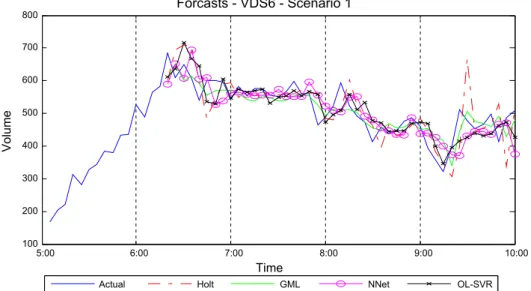
Fig. 1shows the actual and forecasted values for VDS-6. The average percent error (APE) values of these forecasts are shown inFig. 2. See inFig. 2that Holt ES and NNet models clearly pre-sented higher APE values in three different time periods. It can also be noticed in Fig. 2 that, for a period between 9:00 am and 9:25 am, GML does not perform as well as OL-SVR. This is due to the fact that during this time period, the observed traffic flow dif-fers significantly from the average traffic flow observed on the 15-day training period, as shown inFig. 3.
For each VDS, the mean average percent error (MAPE) of each model was computed by simply averaging the APE over the 45 one-step ahead forecasts. The MAPE values in each VDS are shown inTable 3. Notice that the GML approach presented the higher
5:00 6:00 7:00 8:00 9:00 10:00
100 200 300 400 500 600 700 800
Forcasts - VDS6 - Scenario 1
Volume
Time
Actual Holt GML NNet OL-SVR
overall prediction accuracy, with an average MAPE of 5.5%, which supports the findings of previous studies (Lam et al., 2006;Lin, 2001; Tang et al., 2003). Following closely, OL-SVR had the second best overall prediction accuracy, with an average MAPE of 5.9%.Fig. 4shows a plot of the MAPE values presented inTable 3.
5.3. Scenario 2
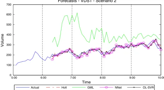
Remember that in this scenario, the prediction models were tested in special days of traffic (holiday on VDS-1 and VDS-5), as well as in days with unexpected occurrences (traffic incident on VDS-3, VDS-4, VDS-6, and VDS-7.Fig. 5shows both actual and pre-dicted values for VDS-1. As expected, notice that the GML-based model had the worst forecasting performance because this model put much more weight on historical values than the other models do. In the case of VDS-1 (4th of July), traffic flows were significantly lower than those observed on the previous days (15 model-calibra-tion days), because home-work trips are not as frequent on the holiday, as illustrated byFig. 6.
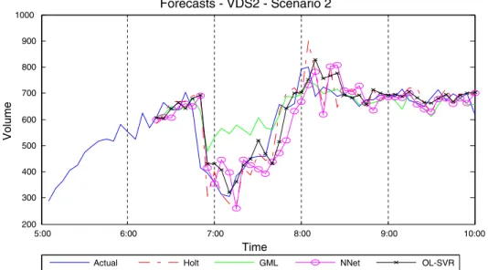
As shown inFig. 7, a traffic incident occurred close to VDS-2 at 6:47 am, blocking traffic until 7:42 am (seeTable 2), which natu-rally dropped the traffic flow recorded on that location. Notice that the other prediction models could respond well to the pattern change, whereas GML, still excessively biased towards the historical values, overestimated the actual flow after the incident
6:20 7:05 7:50 8:35 9:20 10:00
0 5 10 15 20 25 30 35 40 45
Forecast Performance - VDS6 - Scenario 1
APE (%)
Time
Holt GML NNet OL-SVR
Fig. 2.Forecasting performance measured as APE on VDS-6, scenario 1.
6:20 7:05 7:50 8:35 9:20 10:00
300 350 400 450 500 550 600 650 700
VDS6 - Scenario 1
Volume
Time
Historic Current
Fig. 3.Historical flow average (15 days) and current flow (16th day) for VDS 6, scenario 1. Clear discrepancy between historical and current flows exists between 9:00 am and 9:25 am.
Table 3
Forecasting performance – scenario 1
VDS MAPE (%) – scenario 1
Holt ES GML NNet OL-SVR
1 5.4 4.2 5.2 5.1
2 7.7 4.9 7.7 5.4
3 6.5 4.5 8.0 4.8
4 9.8 8.2 9.9 9.0
5 7.0 5.4 6.7 5.1
6 9.6 6.7 8.3 7.1
7 5.8 4.4 5.2 4.6
occurred. This is also shown inFig. 8, where the APE values for VDS-2 are plotted.Fig. 9shows the current and average historical flows. The large discrepancy between the two lines can be seen during the incident time.
For VDS-1 and VDS-5, where the models were tested on a holi-day (4th of July), the MAPE values were calculated based on the whole forecasting period, which was from 6:20 am to 10:00 am. For the other five VDSs, the MAPE values were calculated based on the period that started around 20 min before the occurrence of the incident, and finished around 20 min after the regularity in the traffic flow was achieved. In this way, this research assessed the ability of the models to respond to unexpected changes in the system, as well as their capability to recover their prediction accuracy as traffic returns to its normal pattern.
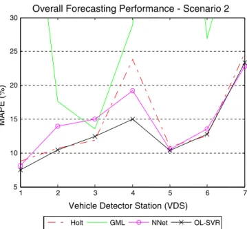
Table 4shows the MAPE values of each model for each VDS in scenario 2. Not surprisingly, the GML-based model presented the lowest prediction performance among all models, with an average MAPE of 40.9%. The OL-SVR model presented the best overall per-formance, with an average MAPE of 13.1%.Fig. 10shows the plot of the MAPE values presented inTable 4.Fig. 11is simply a zoom-in ofFig. 10, to make it easier for the readers to see the results. See in Fig. 10that OL-SVR presented better performance then NNet on
5:00 6:00 7:00 8:00 9:00 10:00
0 100 200 300 400 500 600 700
Forecasts - VDS1 - Scenario 2
Volume
Time
Actual Holt GML NNet OL-SVR
Fig. 5.Actual and predicted values in VDS-1 (holiday), scenario 2. One-step ahead forecasts of 5-min traffic flow from 6:20 am to 10:00 am.
6:20 7:05 7:50 8:35 9:20 10:00
100 200 300 400 500 600 700 800 900
VDS1 - Scenario 2
Volume
Time
Historic Current
Fig. 6.Historical flow average (15 days) and current flow (16th day) for VDS 1 (holiday), scenario 2.
1 2 3 4 5 6 7
0 2 4 6 8 10 12 14
Overall Forecasting Performance - Scenario 1
MAPE (%)
Vehicle Detector Station (VDS)
Holt GLM NNet OL-SVR
5:00 6:00 7:00 8:00 9:00 10:00 200
300 400 500 600 700 800 900 1000
Forecasts - VDS2 - Scenario 2
Volume
Time
Actual Holt GML NNet OL-SVR
Fig. 7.Actual and predicted values in VDS-2 (traffic incident), scenario 2. One-step ahead forecasts of 5-min traffic flow from 6:20 am to 10:00 am.
6:20 7:05 7:50 8:35 9:20 10:00
0 10 20 30 40 50 60 70 80 90 100
Forecast Performance - VDS2 - Scenario 2
APE (%)
Time
Holt GML NNet OL-SVR
Fig. 8.Forecasting performance measured as APE on VDS-2, scenario 2.
6:20 7:05 7:50 8:35 9:20 10:00
300 400 500 600 700 800 900
VDS2 - Scenario 2
Volume
Time
Historic Current
VDS-2, VDS-3, and VDS-4. It also performed better than all models on VDS-4. On the 4th of July (VDS-1 and VDS-5), OL-SVR, Holt ES,
and NNet models had similar overall prediction performance, which was fairly expected as traffic on these two situations were relatively stable and smooth (seeFig. 5), which is advantageous to simple forecasting techniques such as Holt ES.
6. Conclusions and recommendations
This paper proposed an online support vector regression (OL-SVR) approach for the prediction of short-term freeway traffic flow and compared the performance of OL-SVR to other prediction algo-rithms. While the Gaussian maximum likelihood (GML) method Lin, 2001is slightly better for one-step ahead short-term predic-tion under ‘‘normal” or non-incident condipredic-tions, OL-SVR outper-forms GML and other algorithms, such as Holt exponential smoothing and neural net, at some vehicle detection stations (VDS) under atypical conditions such as holidays and incidents.
It should be noted that the prediction of traffic flow under atyp-ical conditions is evidently more challenging than doing so under typical conditions and, hence, much desired by operational agen-cies. Therefore, the proposed OL-SVR is found to be suitable and useful in real-world operations. This advantage is further strength-ened as OL-SVR is inherently fast-paced in its data feeding and ana-lyzing processes.
Future research should look into multivariate time series models that incorporate spatial and temporal correlations among adjacent VDS to improve prediction accuracy, especially when multi-step look-ahead forecasts are desired. In addition, future studies may evaluate the performance of OL-SVR for various look-back intervals, forecasting horizons, and data resolutions. Extension of the work presented herein may address the prediction of other short-term traffic parameters such as average speed and travel time.
Acknowledgements
The authors are thankful to the Freeway Performance Measure-ment System for the availability of the data. The first author appre-ciates the support offered by the Federal Highway Administration’s Eisenhower Graduate Fellowship Program, of which he is proudly a recipient. This work was also partially supported by the National Science Foundation (NSF) grant number CMMI-0644830.
References
Abdulhai, B., Porwal, H., & Recker, W. (2002). Short-term traffic flow prediction using neuro-genetic algorithms.ITS Journal, 7, 3–41.
California Highway Patrol (CHP) (December, 2006) [Online]. <http:// www.chp.ca.gov/index.html>.
Chang, E. C. (1999). Traffic estimation for proactive traffic control.Transportation Research Record, 1679, 81–86.
Chang, C.-C., & Lin, C.-J. (2002). Trainingm-support vector regression: Theory and algorithms.Neural Computation, 14, 1959–1977.
Chen, H., Dougherty, M., & Kirby, H. (2001). The effects of detector spacing on traffic forecasting performance using neural networks. Computer-Aided Civil and Infrastructure Engineering, 16(6), 422–430.
Chen, H., & Grant-Muller, S. (2001). Use of sequential learning for short-term traffic flow forecasting.Transportation Research Part C, 9, 319–336.
Chen, H., Grant-Muller, S., Mussone, L., & Montgomery, F. (2001). A study of hybrid neural network approaches and the effects of missing data on traffic Forecasting.Neural Computing and Applications, 10, 277–286.
Clark, S. (2003). Traffic prediction using multivariate nonparametric regression. Journal of Transportation Engineering, 129(2), 161–168.
Davis, A. G., & Nihan, N. L. (1991). Non-parametric regression and short-term freeway traffic forecasting. Journal of Transportation Engineering, 117(2), 178–188.
De Lurgio, S. A. (1998).Forecasting principles and applications. New York: Irwin/ McGraw Hill, Inc.
Der Voort, M. V., Dougherty, M., & Watson, S. (1996). Combining Kohonen maps with ARIMA time series models to forecast traffic flow.Transportation Research Part C, 4(5), 307–318.
Dia, H. (2001). An object-oriented neural network approach to short-term traffic forecasting.European Journal of Operational Research, 131, 253–261.
Table 4
Overall forecasting performance, scenario 2
VDS MAPE (%) – scenario 2
Holt ES GML NNet OL-SVR
1 8.8 66.0 8.1 7.5
2 10.7 17.6 14.0 10.5
3 11.9 13.6 15.0 12.4
4 23.8 28.9 19.2 15.0
5 10.9 85.8 10.5 10.4
6 12.5 27.0 13.6 12.8
7 24.8 47.4 22.8 23.4
Average 14.8 40.9 14.7 13.1
1 2 3 4 5 6 7
0 10 20 30 40 50 60 70 80 90
Overall Forecasting Performance - Scenario 2
MAPE (%)
Vehicle Detector Station (VDS)
Holt GML NNet O-SVR
Fig. 10.Overall forecasting performance measured as MAPE, scenario 2.
1 2 3 4 5 6 7
5 10 15 20 25 30
Overall Forecasting Performance - Scenario 2
MAPE (%)
Vehicle Detector Station (VDS)
Holt GML NNet OL-SVR
Ding, A., Zhao, X., & Jiad, L. (2002). Traffic flow time series prediction based on statistics learning theory. InProceedings of the IEEE 5th international conference on intelligent transportation systems(pp. 727–730).
Dougherty, M. S., & Cobett, M. R. (1997). Short-term inter-urban traffic forecast using neural networks.International Journal of Forecasting, 13, 21–31. Dreyfus, S. (2005). Neural networks: Methodology and applications. New York:
Springer-Beriln.
Florio, L., & Mussone, L. (1996). Neural-network models for classification and forecasting of freeway traffic flow stability.Control Engineering Practice, 4(2), 153–164.
Freeway Performance Measurement System (PEMS), version 7.0 [Online]. <http:// pems.eecs.berkeley.edu/Public/>.
Hamed, M. M., Al-Masaeid, H. R., & Said, Z. M. (1995). Short-term prediction of traffic volume in urban arterials.Journal of Transportation Engineering, 121(3), 249–254.
Hamed, M. S., & Cook, A. R. (1979). Analysis of freeway traffic time-series data by using Box–Jenkins techniques.Transportation Research Record, 722, 1–9. Ishak, S., & Alecsandru, C. (2004). Optimizing traffic prediction performance of
neural networks under various topological input, and traffic condition settings. Journal of Transportation Engineering, 130(4), 452–465.
Ishak, S., Kotha, P., & Alecsandru, C. (2003). Optimization of dynamic neural network performance for short-term traffic prediction.Transportation Research Record, 1836, 45–56.
Jiang, X., & Adeli, H. (2000). Dynamic wavelet neural network model for traffic flow forecasting. Journal of Transportation Engineering, 131(10), 771–779. 2005.
Kirby, H. R., Watson, S. M., & Dougherty, M. S. (1997). Should we use neural networks or statistical models for short-term traffic forecasting?International Journal of Forecasting, 13, 43–50.
Kwon, E., & Stephanedes, Y. J. (1994). Comparative evaluation of adaptive and neural-network exit demand prediction for freeway control.Transportation Research Record, 1446, 66–76.
Lam, W. H. K., Tang, Y. F., Chan, K. S., & Tam, M.-L. (2006). Short-term traffic flow forecast using Hong Kong Annual Traffic Census. Transportation, 33, 291–310.
Lan, C.-J., & Miaou, S.-P. (1999). Real-time prediction of traffic flows using dynamic generalized linear models.Transportation Research Record, 1678, 168–178. Lee, S., & Fambro, D. (1999). Application of subset autoregressive integrated moving
average model for short-term freeway traffic volume forecasting.Transportation Research Record, 1678, 179–188.
Levin, M., & Tsao, Y.-D. (1980). On forecasting freeway occupancies and volumes. Transportation Research Record, 773, 47–49.
Lin, W.-H. (2001). A Gaussian maximum likelihood formulation for short-term forecasting of traffic flow. InProceedings of the IEEE Intelligent Transportation Systems Conference(pp. 150–155).
Lingras, P., Sharma, S. C., Osborne, P., & Kaylar, I. (2000). Traffic volume time-series analysis according to type of road use.Computer-Aided Civil and Infrastructure Engineering, 15, 365–373.
Ma, J., James, T., & Simon, P. (2003). Accurate online support vector regression. Neural Computation, 15, 2683–2703.
Okutani, I., & Stephanedes, Y. (1984). Dynamic prediction of traffic volume through Kalman filtering theory.Transportation Research – Part B, 18B(1), 1–11. Park, B. (2002). Hybrid neuro-fuzzy application in short-term freeway traffic
volume forecasting.Transportation Research Record, 1802, 190–196.
Park, B., Messer, C. J., & Urbanik, T. II, (1998). Short-term traffic volume forecasting using radial basis function neural network.Transportation Research Record, 1651, 39–47.
Qiao, F., Yu, L., & Wang, X. (2003). Optimizing aggregation level for intelligent transportation system data based on wavelet decomposition.Transportation Research Record, 1840, 10–20.
Qiao, F., Yu, L., & Wang, X. (2004). Double-sided determination of aggregation level for intelligent transportation system data.Transportation Research Record, 1879, 80–88.
Smith, B. L., & Demetsky, M. J. (1995). Short-term traffic flow prediction: Neural network approach.Transportation Research Record, 1453, 98–104.
Smith, B. L., & Demetsky, M. J. (1996). Multiple-interval freeway traffic flow forecasting.Transportation Research Record, 1554, 136–141.
Smith, B. L., & Demetsky, M. L. (1997). Traffic flow forecasting: Comparison of modeling approaches.Journal of Transportation Engineering, 123(4), 261–266. Smith, B. L., Williams, B. M., & Oswald, R. K. (2002). Comparison of parametric and
nonparametric models for traffic flow forecasting.Transportation Research Part C, 10, 302–321.
Stathopoulos, A., & Karlaftis, M. G. (2003). A multivariate state space approach for urban traffic flow modeling and prediction.Transportation Research Part C, 11, 121–135.
Tang, Y. F., Lam, W. K., & Ng, P. L. P. (2003). Comparison of four modeling techniques for short-term AADT forecasting in Hong Kong. Journal of Transportation Engineering, 129(3), 271–277.
Vanajakshi, L., & Rilett, L. R. (2004). A comparison of the performance of artificial neural networks and support vector machines for the prediction of traffic speed. InIEEE intelligent vehicles symposium.
Vapnik, V. (1995). The nature of statistical learning theory. New York: Springer-Verlag.
Vlahogianni, E. I., Karlaftis, M. G., & Golias, J. C. (2005). Optimized and meta-optimized neural networks for short-term traffic flow prediction: A genetic approach.Transportation Research Part C, 13, 211–234.
Williams, B. M., Prya, K. D., & Brown, D. E. (1998). Urban freeway traffic flow prediction. Application of seasonal autoregressive integrated moving average and exponential smoothing models. Transportation Research Record, 1644, 179–188.
Wu, C.-H., Ho, J.-M., & Lee, D. T. (2004). Travel-time prediction with support vector regression. IEEE Transactions on Intelligent Transportation Systems, 5(4), 276–281.
Xiao, H., Sun, H., Ran, B., & Oh, Y. (2003). Fuzzy-neural network traffic prediction framework with wavelet decomposition.Transportation Research Record, 1836, 16–20.
Xiao, H., Sun, H., Ran, B., & Oh, Y. (2004). Special factor adjustment model using fuzzy-neural network in traffic prediction.Transportation Research Record, 1879, 17–23.
Yang, F., Yin, Z., Liu, H. X., & Ran, B. (2004). Online recursive algorithm for short-term traffic prediction.Transportation Research Record, 1879, 1–8.
Yasdi, R. (1999). Prediction of road traffic using a neural network approach.Neural Computation and Application, 8, 135–142.
Yun, S. Y., Namkoong, S., Rho, J. H., Shin, S. W., & Choi, J. U. (1988). A performance evaluation of neural network models in traffic volume forecasting.Mathematical and Computing Modeling, 27(9–11), 293–310.
Zhang, H. M. (2000). Recursive prediction of traffic conditions with neural network models.Journal of Transportation Engineering, 126(6), 472–481.
Zheng, W., Lee, D.-H., & Shi, Q. (2006). Short-term freeway traffic flow prediction: Bayesian combined neural network approach. Journal of Transportation Engineering, 132(2), 114–121.