Thermal Analysis of Satellite Libertad 2: a Guide to CubeSat Temperature Prediction

(1)

xx/xx

J. Aerosp. Technol. Manag., São José dos Campos, v10, e4918, 2018

doi: 10.5028/jatm.v10.1011 ORIGINAL PAPER

1.Universidad Sergio Arboleda – School of Exact Sciences and Engineering – Department of Mathematics – Bogotá/Bogotá – Colombia.

Correspondence author: Alejandro Garzón | Universidad Sergio Arboleda – School of Exact Sciences and Engineering – Department of Mathematics | Calle 74, 14-14 | 110221 – Bogotá/Bogotá – Colombia | Email: alejandro.garzon@correo.usa.edu.com

Received: Jan. 17, 2018 | Accepted: May 24, 2018 Section Editor:Marcia Mantelli

ABSTRACT: We present a model for predicting the temperature of three-unit CubeSat on a low Earth orbit, which supposes a single temperature common to all satellite components. Our exposition includes a detailed, to a large extent analytical, computation of the external heat fluxes for a particular orbit and spacecraft assumptions based on the features foreseen for satellite Libertad 2 under development at Universidad Sergio Arboleda. Moreover, supported by specialized thermal analysis software, we compute the heat fluxes and their associated temperature for all possible orbital orientations, and combine these results with a description of the satellite orbital plane rotation (nodal regression) and the solar motion on the ecliptic, to determine the minima and maxima of the orbital temperature oscillation for a mission lifetime of a year. We find that, for feasible model parameters, the temperature extremes are mostly within the operating temperature range of the most sensitive satellite component, 0 °C ≤ T ≤ 60 °C, suggesting mission viability. Finally, we discuss possible model improvements which would allow testing of satellite design upgrades. In this regard, it is worth noting that the calculation of the external heat fluxes here described can be carried over, almost unchanged, to a more accurate model describing heat transfer between satellite parts with different temperatures.

KEYWORDS: CubeSat, Low Earth orbit, Thermal analysis, Nodal regression, Beta angle, Numerical simulation, Linearization.

INTRODUCTION

The Universidad Sergio Arboleda of Bogotá, Colombia, is building a nano-satellite (for a classification of satellites according to their mass see Fortescue et al. 2003) with the main goal of capturing photographs of Earth’s surface, with potential use in precision agriculture. The satellite, named Libertad 2, will have the shape of a rectangular parallelepided of sides 30 cm × 10 cm × 10 cm (Fig. 1), thus conforming to the CubeSat standard as a three-unit (3U) spacecraft (a description of this standard can be found on The Cubesat Program 2015). Libertad 2 constitutes the continuation of Universidad Sergio Arboleda’s satellite development program started by pico-satellite Libertad 1 (1U, NORAD Catalog Number 31128), launched on April 17, 2007 (Joya 2007; NASA 2014).

The CubeSat standard was developed in 1999 with the objective, among others, of facilitating the involvement of universities in the aerospace industry. This goal could be evaluated as “fulfilled” on the basis of a review by Swartwout (2013), that counted 77 university-led CubeSat-class missions out of a total of 112, between 2000 and 2012. However, the same review reports that university missions have been plagued by a high rate of unsuccessful missions, contributing 27 out of the total 34 failures. Many university missions were also found at the lowest level of mission impact, that of “beepsats”, able only to send basic telemetry. A cause of this situation is lack of training of the teams undertaking CubeSat missions at universities, since the “easy path” to space may have attracted many newcomers. Hence, to channel fruitfully this interest, it is urgent to develop resources for a rapid

Thermal Analysis of Satellite Libertad 2: a

Guide to CubeSat Temperature Prediction

Alejandro Garzón1_{, Yovani A. Villanueva}1

Garzón A; Villanueva YA (2018) Thermal Analysis of Satellite Libertad 2: a Guide to CubeSat Temperature Prediction. J Aerosp Technol Manag, 10:e4918. doi: 10.5028/jatm. v10.1011.

How to cite

Garzón A http://orcid.org/0000-0003-0069-7306

(2)

J. Aerosp. Technol. Manag., São José dos Campos, v10, e4918, 2018 Garzón A; Villanueva YA

xx/xx 02/24

and low-cost acquisition of the pertinent aerospace education. Failing to do so, we may be defeating one of the purposes of the CubeSat standard by accepting that relevant CubeSat missions are the sole privilege of well-established institutions (universities, government organizations, or businesses) of the aerospace sector. An example of a CubeSat mission by experienced developers is the Dynamic Ionosphere CubeSat Experiment (DICE) (Fish et al. 2014); a growing interest of commercial developers in nano-satellites was reported by Buchen (2014).

Figure 1. Views of Libertad 2 with the body fixed coordinate system {x,y,z}. The faces are labeled by a numerical index and a word. The front face has dimensions 10 cm × 10 cm and the bottom face is 10 cm × 30 cm.The dark gray hexagons represent

solar cells while the light gray circle represents the camera lens opening. x

y

z x

y z

(1, front)

(2, bottom)

(3,left)

(6, rear) (4, top)

(5, right)

Acknowledging this need, this paper intends to be a resource for quick learning of the concepts and methods involved in predicting the temperature of a CubeSat. Necessary background material is included to make the presentation self-contained, model assumptions are given a clear mathematical formulation, and the computations feature intermediate steps to facilitate their reproduction, thereby making the paper accessible to anyone with a solid quantitative training.

Prediction of a satellite’s temperature is justified by the need for all satellite components to function within their operating temperature ranges – defined as “the maximum and minimum temperature limits between which components successfully and reliably meet their specified operating requirements” (Garzon 2012) –, otherwise risking malfunctioning or damage. To forecast the effect of design choices, like the materials on the external surfaces, on the temperature, it is necessary to create a model of the heat transferred between the satellite and its surroundings and between the satellite parts.

The modeling techniques can be found in the available literature on thermal analysis of nano-satellites. Dinh (2012) studied the temperature of internal electronics in a 1U CubeSat using the software packages Thermal Desktop and ANSYS. Jacques (2009) conducted the thermal analysis for the OUFTI-1U CubeSat relying on the software ESATAN-TMS, whereas Garzon (2012) simulated the temperatures of the OSIRIS-3U CubeSat employing the multiphysics software COMSOL. Bulut and Sozbir (2015) investigated the temperature for different solar panel combinations in a 1U CubeSat. Optimization of thermal design parameters through genetic algorithms was pursued by Escobar et al. (2016). Kang and Oh (2016) performed an experimental validation of their model predictions using a thermal vacuum chamber. Active thermal control with phase change materials was investigated by Shinde et al. (2017) and Kang and Oh (2016). A simulation code implemented in MATLAB was developed by Corpino

et al. (2015). Mason et al. (2018) compared a thermal model of the Miniature X-Ray Solar Spectrometer 3U CubeSat with actual on-orbit temperature measurements, finding agreement within a few degrees Celsius. Remarkably, their thermal design allowed for the payload to stay at an almost constant on-orbit temperature of –40.91 °C (standard deviation of 0.19 °C), isolated from the much wider temperature oscillations of the solar arrays, roughly from –40 °C to 50 °C.

(3)

J. Aerosp. Technol. Manag., São José dos Campos, v10, e4918, 2018 Thermal Analysis of Satellite Libertad 2: a Guide to CubeSat Temperature Prediction

xx/xx 03/24

single temperature model (also known as a single node model), serves as a stepping stone toward the development of a more accurate, multiple node model (with different parts allowing different temperatures), which will be the subject of a future work. In particular, the irradiances associated to the external heat sources, here presented, can be passed unchanged to the multiple node model.

This study is structured as follows. In the section Design of Libertad 2, the satellite components and their operating temperature ranges are presented. The following section introduces the single node model for a special orbit and shows the model-predicted temperature (model solutions) together with some verification criteria. Then, the variation of the external heat fluxes over a mission life of a year is considered; the resulting effect on the satellite temperature is computed with the help of the thermal analysis software ESATAN-TMS release 5. Finally, the last section summarizes our results and discusses possible future work.

DESIGN OF LIBERTAD 2

The satellite will carry several components in addition to the photographic camera. A system of wheels and electromagnets will control the satellite orientation for the purpose of pointing the camera toward a particular target. These actuators together with orientation sensors constitute what is known as the Attitude Determination and Control System (ADCS). Instructions will be sent to the satellite via Very High Frequency (VHF) and Ultra High Frequency (UHF) radio waves. S-Band microwaves will be used to transmit the photographs as digital data. Hence, the satellite will have transmitter and receiver equipment on the above mentioned telecommunication bands (named, respectively, VHF-UHF transceiver and S-band transceiver). Solar cells will provide the satellite energy, part of which will be stored in a battery (to provide energy in the periods of low or nil solar radiation, for instance, when the satellite traverses Earth’s shadow), that will be distributed between the previously referred components by a special circuitry, the Electric Power System (EPS). The processing of instructions and the coordination of all the components tasks will be performed by an On Board Computer (OBC).

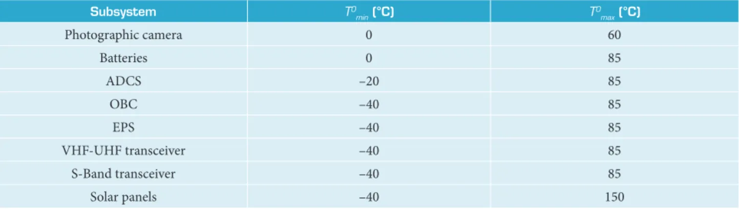
Table 1 shows the operating temperature range (TO min, T

O

max), for each satellite subsystem. Operation outside these ranges should be avoided.

Table 1. Operating minimum and maximum temperature values (TO min and T

O

max, respectively) for the satellite subsystems.

Subsystem TO

min (°C) T

O max (°C)

Photographic camera 0 60

Batteries 0 85

ADCS –20 85

OBC –40 85

EPS –40 85

VHF-UHF transceiver –40 85

S-Band transceiver –40 85

Solar panels –40 150

SINGLE NODE MODEL

(4)

xx/xx 04/24

Satellite Libertad 2 will be put on an orbit with altitude in the range 600 – 900 km, which fits into the definition of a Low Earth Orbit (LEO), according to Vallado (1997). At this altitude, the most significant heat fluxes entering the i-th satellite face (cf. Fig. 1 for a labeling of the faces) are Q_S,i(t), Q_alb,i(t), and Q_E,i(t), whose sources are, respectively, the direct solar radiation, the solar radiation reflected on the surface of Earth (albedo radiation), and the infrared radiation emitted by Earth (Fortescue 2003; Gilmore 2002). For the outgoing heat flux, we assume that the i-th satellite face emits infrared radiation as a gray body, with radiosity ε_iσT4_{, where}

_ε

i is the face’s emissivity, 0 <

ε

i < 1, a property of the face’s surface finish, and σ is the Stefan-Boltzmann’s constant. Combining the previous assumptions leads to the following evolution equation for the temperature T (Eq. 1),

ε σ

ε

σ

𝐶𝐶

𝑑𝑑𝜎𝜎

_{𝑑𝑑𝑡𝑡 = −𝜎𝜎𝐴𝐴}

)**

𝜎𝜎

+

+ 𝑄𝑄

./.

(𝑡𝑡),

𝐴𝐴

)**

= 3 𝐴𝐴

4

𝜀𝜀

4 6

478

𝑄𝑄

./.

(𝑡𝑡) = 𝑄𝑄

9

(𝑡𝑡) + 𝑄𝑄

:;<

(𝑡𝑡) + 𝑄𝑄

=

(𝑡𝑡)

𝑄𝑄

9

(𝑡𝑡) = ∑ 𝑄𝑄

6478 9,4

(𝑡𝑡)

𝑄𝑄

:;<

(𝑡𝑡) = ∑ 𝑄𝑄

6478 :;<,4

(𝑡𝑡)

𝑄𝑄

=

(𝑡𝑡) = ∑ 𝑄𝑄

6478 =,4

(𝑡𝑡)

ε σ

ε

σ

𝐶𝐶

𝑑𝑑𝜎𝜎

_{𝑑𝑑𝑡𝑡 = −𝜎𝜎𝐴𝐴}

)**

𝜎𝜎

+

+ 𝑄𝑄

./.

(𝑡𝑡),

𝐴𝐴

)**

= 3 𝐴𝐴

4

𝜀𝜀

4 6

478

𝑄𝑄

./.

(𝑡𝑡) = 𝑄𝑄

9

(𝑡𝑡) + 𝑄𝑄

:;<

(𝑡𝑡) + 𝑄𝑄

=

(𝑡𝑡)

𝑄𝑄

9

(𝑡𝑡) = ∑ 𝑄𝑄

6478 9,4

(𝑡𝑡)

𝑄𝑄

:;<

(𝑡𝑡) = ∑ 𝑄𝑄

6478 :;<,4

(𝑡𝑡)

𝑄𝑄

=

(𝑡𝑡) = ∑ 𝑄𝑄

6478 =,4

(𝑡𝑡)

ε σ

ε

σ

𝐶𝐶

𝑑𝑑𝜎𝜎

_{𝑑𝑑𝑡𝑡 = −𝜎𝜎𝐴𝐴}

)**

𝜎𝜎

+

+ 𝑄𝑄

./.

(𝑡𝑡),

𝐴𝐴

)**

= 3 𝐴𝐴

4

𝜀𝜀

4 6

478

𝑄𝑄

./.

(𝑡𝑡) = 𝑄𝑄

9

(𝑡𝑡) + 𝑄𝑄

:;<

(𝑡𝑡) + 𝑄𝑄

=

(𝑡𝑡)

𝑄𝑄

9

(𝑡𝑡) = ∑ 𝑄𝑄

6478 9,4

(𝑡𝑡)

𝑄𝑄

:;<

(𝑡𝑡) = ∑ 𝑄𝑄

6478 :;<,4

(𝑡𝑡)

𝑄𝑄

=

(𝑡𝑡) = ∑ 𝑄𝑄

6478 =,4

(𝑡𝑡)

ε σ

ε

σ

𝐶𝐶

𝑑𝑑𝜎𝜎

_{𝑑𝑑𝑡𝑡 = −𝜎𝜎𝐴𝐴}

)**

𝜎𝜎

+

+ 𝑄𝑄

./.

(𝑡𝑡),

𝐴𝐴

)**

= 3 𝐴𝐴

4

𝜀𝜀

4 6

σ

𝐶𝐶

𝑑𝑑𝜎𝜎

_{𝑑𝑑𝑡𝑡 = −𝜎𝜎𝐴𝐴}

)**

𝜎𝜎

+

+ 𝑄𝑄

./.

(𝑡𝑡),

𝐴𝐴

)**

= 3 𝐴𝐴

4

𝜀𝜀

4 6

478

𝑄𝑄

./.

(𝑡𝑡) = 𝑄𝑄

9

(𝑡𝑡) + 𝑄𝑄

:;<

(𝑡𝑡) + 𝑄𝑄

=

(𝑡𝑡)

𝑄𝑄

9

(𝑡𝑡) = ∑ 𝑄𝑄

6478 9,4

(𝑡𝑡)

𝑄𝑄

:;<

(𝑡𝑡) = ∑ 𝑄𝑄

4786 :;<,4

(𝑡𝑡)

and

𝑄𝑄

=

(𝑡𝑡) = ∑ 𝑄𝑄

6478 =,4

(𝑡𝑡)

.

(1)

(2)

(3)

where (Eq. 2),

with A_i the area of the i-th face, and Q_tot(t) is the total external heat flux (Eq. 3),

with and

The heat fluxes Q_S,i(t), Q_alb,i(t), and Q_E,i(t) depend on the satellite orbit and orientation, with Q_S,i(t) and Q_alb,i(t) further affected by the direction of the sunrays, denoted by the (unit) solar vector ŝ, which points toward the sun. In the following sections we show, in a special case, how these factors enter the computation of the heat fluxes.

SATELLITE ORBIT, SATELLITE ATTITUDE, AND SOLAR VECTOR

The satellite orbit is described in relation to the Geocentric Equatorial Coordinate System (GECS) (Vallado1997) with origin at Earth’s center and axes {X, Y, Z}, with unit vectors {û₁, û₂, û₃}, oriented as follows. û₃points toward the North Pole (Fig. 2), while û₁ and û₂ are contained in the plane of Earth’s equator and have fixed directions (described in the next section) in relation to the distant stars.

Figure 2. Satellite orbit and orientation in relation to the Geocentric Equatorial Coordinate System {û₁, û₂, û₃}.

u

x

y z

x

y z

x y z

ˆ

3

u ˆ₂ u

(5)

xx/xx 05/24

Throughout the paper, we assume for Libertad 2 a perfectly circular orbit of radius R = 7110 km (similar to the orbit of Libertad 1, discussed in the next section). In this section, the orbit is supposedly in the û₁ – û₃ plane (Fig. 2) and the solar vector is taken as ŝ = û₁. General orbital planes and ŝ are considered in the following sections.

The satellite’s orientation (or attitude) is described in terms of a body fixed coordinate system {x, y, z}, with unit vectors {ê₁, ê₂, ê₃}, oriented with respect to the satellite as shown in Fig. 1. The camera’s optical axis will be parallel to ê₁ and the lens will look through an orifice on face 2. A satellite on a LEO is subject to atmospheric drag that reduces the satellite’s kinetic energy causing it to eventually fall on Earth. To minimize atmospheric friction, the satellite’s longer edges, parallel to ê₃, will be aligned with the satellite’s velocity. The vector –ê₁ will point toward the center of Earth (–ê₁ parallel to nadir) to enable the camera to photograph the globe’s surface. This orientation scenario (Fig. 2), which we label as velocity-nadir attitude, could be maintained throughout the entire orbit, despite external torques, thanks to the ADCS.

For quick face identification, we find it convenient to use a word labeling (Fig. 1), alternative to the index i, based on the mnemonic of imagining the satellite as a miniature land vehicle with the vector from the rear to the windshield parallel to the velocity and its bottom looking toward Earth.

Having specified the orbit and satellite orientation, we proceed to the calculation of the incoming heat fluxes.

CALCULATION OF DIRECT SOLAR RADIATION

Figure 3 shows the satellite on its orbit as viewed from the –û₂ direction. An arc of the orbit, with angle measure 2ξ, given by (Eq. 4),

ξ

𝜉𝜉 = sin

D8

_(𝑅𝑅

=

/𝑅𝑅) ≈ 63.8°

𝒏𝒏N

4

ŝ

cos 𝑏𝑏

4

= 𝒏𝒏N

4

∙ 𝒔𝒔T

.

ξ

≤

4

∙ 𝒔𝒔T

𝒏𝒏N

4

ŝ

𝒏𝒏N

+

=

𝒆𝒆T

8

= cos 𝜈𝜈 𝒖𝒖N

8

+ sin 𝜈𝜈 𝒖𝒖N

Z

cos 𝑏𝑏

+

= 𝒏𝒏N

+

∙ 𝒔𝒔T = cos 𝜈𝜈

cos 𝑏𝑏

4

= 𝒏𝒏N

4

∙ 𝒔𝒔T

ξ

≤

4

ŝ

𝒏𝒏N

+

=

𝒆𝒆T

8

= cos 𝜈𝜈 𝒖𝒖N

8

+ sin 𝜈𝜈 𝒖𝒖N

Z

cos 𝑏𝑏

+

= 𝒏𝒏N

+

∙ 𝒔𝒔T = cos 𝜈𝜈

(4)

(5)

(6)

with R_E = 6378 km (Bate et al. 1971) the radius of Earth, passes through the shadow projected by Earth (eclipse zone) where the direct solar radiation heat fluxes (solar heat fluxes, for short) Q_S,i are zero. Outside the eclipse zone, Q_S,i will depend on the angle

b_i between the outward unit vector normal to the face, n ˆ_i , and the solar vector ŝ (Eq. 5)

cos b_i≤ 0 means the sunrays do not reach the face, so, also in this case, Q_S,i = 0. When cos b_i > 0, the face will project, onto a plane perpendicular to the solar rays, an area A cos b_i, absorbing a heat flux (Eq. 6)

where α_i is the face’s absorptivity, 0 < α_i < 1 which, as the emissivity, is a property of the face’s external surface finish, and I_S is the solar irradiance (the energy transported by the solar radiation per unit of area and unit of time). The solar irradiance I_S depends on the satellite-sun distance, implying that, for a LEO, I_S is highest (lowest) at perihelion (aphelion). In this work we use the recommended mean value, known as the solar constant, I_S = 1367 W/m2_(Anderson_{et al.}_{2001), thus neglecting the variation of}

I_S around this mean (±3.4%).

The angle b_i will be determined by the satellite position on the orbit, denoted by the true anomaly v, measured from the û₁ direction (Fig. 3). To calculate the product n ˆ_i_∙s ŝ we express both n ˆ_i and ŝ in the {û₁, û₂, û₃} basis. Therefore, for the top face, we have n ˆ₄ = e ˆ₁ = cos vu ˆ₁ + sin vu ˆ₃. So, cos b₄=n ˆ₄_∙s ŝ = cos v. Similar calculations apply to the remaining faces.

Faces left, right and space will be partially covered by six solar cells (Fig. 1), each cell with an area of 30.18 cm2_(AZUR

(6)

xx/xx 06/24

where f_c = 60.36% is the fraction of the face’s area covered by solar cells, and α_u = 0.5 is the absorptivity of the non-solar-cell surfaces, yielding α_avg = 0.578.

Figure 3. Satellite orbit as viewed from the –û₂ direction (see Fig. 2 for the coordinate system definition). The dark gray region represents the orbit eclipse zone. ξ is half the angle measure of the eclipse zone and v is the true anomaly.

ξ ξ

rsat

v

ν _û

1

û₃

R_E

R

η

α

η

α

𝛼𝛼

:[\

= 𝑓𝑓

^

𝛼𝛼

)**

+ (1 − 𝑓𝑓

^

)𝛼𝛼

`

,

α

𝑄𝑄

9

= ∑

6478

𝑄𝑄

9,4

ξ

≤ ≤

ξ

ω

𝜈𝜈(𝑡𝑡) = 𝜈𝜈

a

+ 𝜔𝜔𝑡𝑡

η

α

η

α

𝛼𝛼

:[\

= 𝑓𝑓

^

𝛼𝛼

)**

+ (1 − 𝑓𝑓

^

)𝛼𝛼

`

α

𝑄𝑄

9

= ∑

6478

𝑄𝑄

9,4

ξ

≤ ≤

ξ

ω

𝜈𝜈(𝑡𝑡) = 𝜈𝜈

a

+ 𝜔𝜔𝑡𝑡

,

(7)

(8)

(9)

Figure 4. Total solar heat flux QS (solid line) and total albedo heat flux Qalb (dashed line) as functions of the true anomaly v. Both QS and Qalb fall to zero inside the eclipse zone, 180° –ξ ≤ v≤ 180° + ξ (see Fig. 3).

0 90 180 270 360

0 10 20

ν (o₎

Qs

, Q

alb

(W

)

Figure 4, shows the total solar heat flux as function of the true anomaly v.

By considering the variation in time of v, we can express the heat fluxes as functions of time, Q_S,i(t) = Q_S,i[v(t)]. For a circular orbit, the true anomaly changes with constant angular velocity ω (Eq. 8),

where the initial value is chosen for convenience as v₀ = 0 and ω is given by Kepler’s third law (Vallado 1997) (Eq. 9),

ω

𝜔𝜔 = c

_𝑅𝑅

𝜇𝜇

_Z

,

×

𝑃𝑃 =

2𝜋𝜋

_{𝜔𝜔 ≈ 99.4 min.}

θ ϕ

θ

ϕ

(7)

xx/xx 07/24

CALCULATION OF INFRARED RADIATION

The Earth emits thermal radiation with highest values of the spectral distribution inside the infrared wavelength band (Anderson

et al. 2001; Anderson and Smith 1994). A patch on the surface of Earth is approximated as a perfectly diffuse radiator (Palmer and Grant 2010; Wolfe 1998) with radiosity I_E, defined as the radiant flux leaving the patch per unit area. I_E is higher (lower) in warmer (colder) areas of the globe and clouds absorb infrared radiation, decreasing the value of I_E perceived by a spacecraft on orbit (Anderson et al. 2001; Anderson and Smith 1994). As a result, I_E changes both in space and time, I_E = I_E(θ, ϕ, t), where θ

and ϕ are angular coordinates describing a point on the surface of Earth. However, for the sake of simplicity, I_E may be modeled as uniform over the globe, I_E = I_E(t), with the time-variation taking into account the change of the part of the globe viewed by the satellite as it traverses its orbit, as well as the intrinsic time-fluctuation of I_E.

During the Earth Radiation Budget Experiment (ERBE) the infrared radiation falling over three LEO satellites was recorded every 16 s during 28 months (Anderson et al. 2001; Anderson and Smith 1994). The infrared intensity was reported as the radiosity I_E(t) of a spherical surface at an altitude of 30 km above the surface of the Earth, termed Top of Atmosphere (TOA). The measured I_E(t) changed erratically and was treated as a random time series. For orbits of inclination above 60° (see the next section for the definition of inclination) a time-averaged I_E-value of 211 W/m2_{was found (Anderson}_{et al.}_{2001). In this work, we assume a}

spatially uniform time-constant radiosity I_E equal to this mean, scaled following conservation of energy from TOA to the surface of Earth by the factor (R_E + 30 km)2_{/, yielding the final value of}_I

E = 213 W/m

2_.

Due to the uniformity and time-invariance of I_E, the Earth heat fluxes Q_E,i are independent of the satellite position on its orbit, thus constant in time. Conforming to Lambert’s law, a surface element on the globe of area dS will emit, in the direction of the satellite, a radiant intensity (power per solid angle) I_Ecos a_E dS/π, where a_E is the angle between the unit vector pointing from the surface element toward the satellite ˆ ρ and the unit vector normal to the surface element ˆ n_E (see Fig. 5). The i-th face will intercept the radiant energy traveling in a solid angle A_i cos a_i/ρ2_{, with}_a

i the angle between – ˆ ρ and nˆ i. Of this energy a fraction εi will be absorbed. As a result, the contribution of the surface element to the heat flux Q_E,i is (Eq. 11),

(10)

(11)

(12)

(14) (13)

Integrating over all surface elements yields (Eq. 12),

where F_iE is the radiative view factor (Eq. 13),

To evaluate the integral in (Eq. 13), we express it in spherical coordinates (r, θ, ϕ), with û₃ acting as the z-axis. We begin recalling that cos a_E = ˆ ρ · ˆ n_Eand cos a_i = – ˆ ρ · ˆ n_i. Next, we define ρ = r_sat – r_E, where r_sat is the satellite position and r_E is the surface element position (Eq. 14),

Therefore, ρ = ||ρ|| , ρρ = ˆ ρ/ρ, and ˆ n_E= r_E/R_E. The view factor F_iE is independent of the true anomaly v. Hence, for ease, we chose r_sat = Rû₃. As an example, we compute F_iE for the bottom face, F₂_E, in which case, ˆ n_i= –û₃. Substituting the previous vector relationships into (Eq. 13) leads to (Eq. 15),

𝑅𝑅=

k

π

𝝆𝝆N

𝒏𝒏N=

ρ

−𝝆𝝆N

𝒏𝒏N4

ε

𝑑𝑑𝑄𝑄=,4

= 𝜀𝜀4

𝐴𝐴4𝐼𝐼=

cos 𝑎𝑎=

_{𝜋𝜋𝜌𝜌}

cos 𝑎𝑎4

_k

𝑑𝑑𝑑𝑑.

𝑄𝑄

=,4

= 𝜀𝜀

4

𝐴𝐴

4

𝐼𝐼

=

𝐹𝐹

4=

,

𝐹𝐹

4=

= q

cos 𝑎𝑎

= −𝝆𝝆N ⋅

𝒏𝒏N

4

ρ

𝒓𝒓

=

= 𝑅𝑅

=

(sin 𝜃𝜃 cos 𝜙𝜙 𝒖𝒖N

8

+ sin 𝜃𝜃 sin 𝜙𝜙 𝒖𝒖N

k

+ cos 𝜃𝜃 𝒖𝒖N

Z

)

ρ

𝝆𝝆N

ρ

𝒏𝒏N

=

𝒏𝒏N

4

𝑄𝑄

=,4

= 𝜀𝜀

4

𝐴𝐴

4

𝐼𝐼

=

𝐹𝐹

4=

,

𝐹𝐹

4=

= q

cos 𝑎𝑎

= −𝝆𝝆N ⋅

𝒏𝒏N

4

ρ

𝒓𝒓

=

= 𝑅𝑅

=

(sin 𝜃𝜃 cos 𝜙𝜙 𝒖𝒖N

8

+ sin 𝜃𝜃 sin 𝜙𝜙 𝒖𝒖N

k

+ cos 𝜃𝜃 𝒖𝒖N

Z

)

ρ

𝝆𝝆N

ρ

𝒏𝒏N

=

𝒏𝒏N

4

𝑄𝑄

=,4

= 𝜀𝜀

4

𝐴𝐴

4

𝐼𝐼

=

𝐹𝐹

4=

,

𝐹𝐹

4=

= q

cos 𝑎𝑎

= −𝝆𝝆N ⋅

𝒏𝒏N

4

4

ω

𝜔𝜔 = c_𝑅𝑅𝜇𝜇_Z ,

×

𝑃𝑃 =2𝜋𝜋_{𝜔𝜔 ≈ 99.4 min.}

(8)

xx/xx 08/24

where h = R/R_Eand the limit of integration θ < θ_M, with θ_M= cos–1₍_R

E/R), is determined by the condition cos aE> 0, which states that infrared rays do not traverse the Earth. Evaluation of Eq. 15 yields (Eq. 16),

Figure 5. Quantities involved in the calculation of the infrared heat flux over the i-th satellite face, Q_iE (Eqs. 12 and 13). (15)

(16)

(17)

(18)

For faces front, rear, left and right (i = 1,3,5,6), evaluation of Eq. 13 yields (Eq. 17)

We assume an emissivity

ε

u = 0.05, corresponding to a shiny metallic surface finish (Gilmore 2002), for all surfaces not covered by solar cells (this includes the totality of the faces devoid of solar cells). Hence, the faces that do possess solar cells will display average emissivity (Eq. 18),

where

ε

C = 0.89 is the solar cells’ emissivity (AZUR SPACE 2014), so

ε

avg = 0.557.

Table 2 presents the value of Q_E,i calculated for each face.

Table 2. Infrared heat fluxes Q_E,i computed using Eq. 12 and the program ESATAN. The table total corresponds to Q_E= ∑ 6

i = 1QE,i

Face QE,i(W)

Eq.12 ESATAN

Front 0.0243 0.0242

Bottom 0.2571 0.2585

Left 0.8119 0.8006

Top 0 0

Right 0.8119 0.8404

Rear 0.0243 0.0247

Total 1.9294 1.9484

nE n_i ρ a_E a_i ˆ ^ ^ ^

𝐹𝐹

k=

=

_𝜋𝜋

1 q q

(1 − ℎ cos 𝜃𝜃)(cos 𝜃𝜃 − ℎ)

_{(1 + ℎ}

k

_{− 2ℎ cos 𝜃𝜃 )}

k

sin 𝜃𝜃𝑑𝑑𝜙𝜙𝑑𝑑𝜃𝜃,

kw

a xy

a

θ θ

θ

𝐹𝐹

k=

=

_ℎ

1

_k

≈ 0.80.

𝐹𝐹

4=

= −

√ℎ

k

_{− 1}

𝜋𝜋ℎ

k

+

1 𝜋𝜋 tan

D8

~

1 √ℎ

k

_{− 1}

,

≈ 0.23.

ε

k=

=

_𝜋𝜋

1 q q

(1 − ℎ cos 𝜃𝜃)(cos 𝜃𝜃 − ℎ)

_{(1 + ℎ}

k

_{− 2ℎ cos 𝜃𝜃 )}

k

sin 𝜃𝜃𝑑𝑑𝜙𝜙𝑑𝑑𝜃𝜃,

kw

a xy

a

θ θ

θ

𝐹𝐹

k=

=

kw

a xy

a

θ θ θ

𝐹𝐹k==_ℎ1k≈ 0.80.

𝐹𝐹4= = −√ℎ

k_{− 1}

𝜋𝜋ℎk +

1

𝜋𝜋 tanD8~

1

√ℎk_{− 1},

≈ 0.23.

ε

𝜀𝜀:[\ = 𝑓𝑓^𝜀𝜀^+ (1 − 𝑓𝑓^)𝜀𝜀`

ε ε

𝐹𝐹k==1_𝜋𝜋q qkw(1 − ℎ cos 𝜃𝜃)(cos 𝜃𝜃 − ℎ)_{(1 + ℎ}_k_{− 2ℎ cos 𝜃𝜃 )}_k sin 𝜃𝜃𝑑𝑑𝜙𝜙𝑑𝑑𝜃𝜃,

a xy

a

θ θ θ

𝐹𝐹k==_ℎ1k≈ 0.80.

𝐹𝐹4= = −√ℎ_𝜋𝜋ℎk− 1_k +1_{𝜋𝜋 tan}D8_~ 1

√ℎk_{− 1},

≈ 0.23.

ε

𝜀𝜀:[\= 𝑓𝑓^𝜀𝜀^+ (1 − 𝑓𝑓^)𝜀𝜀`

ε ε

𝐹𝐹k==1_𝜋𝜋q qkw(1 − ℎ cos 𝜃𝜃)(cos 𝜃𝜃 − ℎ)_{(1 + ℎ}_k_{− 2ℎ cos 𝜃𝜃 )}_k sin 𝜃𝜃𝑑𝑑𝜙𝜙𝑑𝑑𝜃𝜃,

a xy

a

θ θ θ

𝐹𝐹k==_ℎ1_k≈ 0.80.

𝐹𝐹4= = −√ℎ_𝜋𝜋ℎk− 1_k +1_{𝜋𝜋 tan}D8_~ 1

√ℎk_{− 1},

≈ 0.23.

ε

𝜀𝜀:[\= 𝑓𝑓^𝜀𝜀^+ (1 − 𝑓𝑓^)𝜀𝜀`

(9)

xx/xx 09/24

CALCULATION OF REFLECTED SOLAR RADIATION

We suppose that a patch on the surface of Earth reflects light diffusely and equally in all directions (Lambertian reflectance) with diffuse reflectance (also known as albedo) γ, defined as the reflected fraction of the incident radiant flux. More accurate models use the bidirectional reflectance distribution function (Schaepman-Strub et al. 2006), employed, for instance, in processing the data provided by NASA’s MODIS Instruments on board the Aqua and Terra satellites (NASA 2015; Strahler et al. 1999). The albedo varies considerably across the globe: it is usually higher over areas covered with ice and snow, deserts, and cloudy regions, and generally lower over the oceans, in the absence of clouds (Anderson et al. 2001; Anderson and Smith 1994). Therefore, the albedo depends on place and time, γ = γ(θ, ϕ, t), but, for simplicity, it is modeled as if it were uniform, γ = γ(t). The albedo γ(t) of the TOA measured during the ERBE behaved like a random time series (as did I_E(t)) with a mean value of 0.23 for orbits of inclination superior to 60° (Anderson et al. 2001). In this work, we assume for γ a time-constant value equal to this mean plus the correction for zero β angle (see the next section for the definition of the β angle) of 0.04 found in Anderson et al. (2001), scaled from the TOA to the surface of Earth, for a final value of γ = 0.273.

For the calculation of the albedo radiation heat fluxes, we follow Fitz et al. (1963). An element on the surface of Earth, of area

dS, diffusely reflecting solar radiation may be considered as a diffuse radiator with radiosity cos (b_E) γI_S, where b_E is the angle between the normal to the surface element ˆ _n

E and the solar vector ŝ (Eq. 19),

(19) (20) (21) (22) (23) (24)

γ

β

γ

𝒏𝒏N=

ŝ

cos(𝑏𝑏=) = 𝒏𝒏N=

cos 𝑏𝑏=

𝑑𝑑𝑑𝑑.

𝑄𝑄:;<,4

= 𝛼𝛼4𝐴𝐴4𝛾𝛾𝐼𝐼9 𝐹𝐹Å

4= ,

𝐹𝐹Å

4=

γ

β

γ

𝒏𝒏N=

ŝ

cos(𝑏𝑏=) = 𝒏𝒏N=

∙ 𝒔𝒔T.

γ

ε

α

𝑑𝑑𝑄𝑄:;<,4

= 𝛼𝛼4𝐴𝐴4𝛾𝛾𝐼𝐼9

cos 𝑎𝑎=

cos 𝑎𝑎4

_{𝜋𝜋𝜌𝜌}

_k

cos 𝑏𝑏=

𝑑𝑑𝑑𝑑.

𝑄𝑄:;<,4

= 𝛼𝛼4𝐴𝐴4𝛾𝛾𝐼𝐼9 𝐹𝐹Å4= ,

𝐹𝐹Å4=

𝐹𝐹Å

4=

= q

cos 𝑎𝑎

=

cos 𝑎𝑎

_{𝜋𝜋𝜌𝜌}

_k4

cos 𝑏𝑏

=

𝑑𝑑𝑑𝑑.

{𝒆𝒆T

8É

, 𝒆𝒆T

kÉ

, 𝒆𝒆T

ZÉ

}

𝒆𝒆T

ZÉ

𝒔𝒔T = sin 𝜈𝜈 𝒆𝒆T

₈É

_{+ cos 𝜈𝜈 𝒆𝒆T}

Z É

_.

{𝒆𝒆T

₈É

_{, 𝒆𝒆T}

k É

_{, 𝒆𝒆T}

Z

É

_}

_{θ ϕ}

𝒆𝒆T

ZÉ

𝐹𝐹Å

k=

(𝜈𝜈) =

1 _𝜋𝜋

q q

(1 − ℎ cos 𝜃𝜃)(cos 𝜃𝜃 − ℎ)

_{(1 + ℎ}

_k

_{− 2ℎ cos 𝜃𝜃 )}

_k ÖÜ(x)

xy

xá

×

(sin 𝜃𝜃 cos 𝜙𝜙 sin 𝜈𝜈 + cos 𝜃𝜃 cos 𝜈𝜈) sin 𝜃𝜃 𝑑𝑑𝜙𝜙𝑑𝑑𝜃𝜃,

θ

ϕ

θ

ℛ

θ ϕ

θ

≤ θ

θ

𝐹𝐹Å

4=

= q

cos 𝑎𝑎

=

cos 𝑎𝑎

_{𝜋𝜋𝜌𝜌}

_k4

cos 𝑏𝑏

=

𝑑𝑑𝑑𝑑.

{𝒆𝒆T

₈É

_{, 𝒆𝒆T}

k É

_{, 𝒆𝒆T}

Z

É

_}

_𝒆𝒆T

Z É

𝒔𝒔T = sin 𝜈𝜈 𝒆𝒆T

8É

+ cos 𝜈𝜈 𝒆𝒆T

ZÉ

.

{𝒆𝒆T

8É

, 𝒆𝒆T

kÉ

, 𝒆𝒆T

ZÉ

}

θ ϕ

𝒆𝒆T

_ZÉ

𝐹𝐹Å

k=(𝜈𝜈) =

1 _𝜋𝜋

q q

(1 − ℎ cos 𝜃𝜃)(cos 𝜃𝜃 − ℎ)

_{(1 + ℎ}

_k

_{− 2ℎ cos 𝜃𝜃 )}

_k ÖÜ(x)

xy

xá

×

(sin 𝜃𝜃 cos 𝜙𝜙 sin 𝜈𝜈 + cos 𝜃𝜃 cos 𝜈𝜈) sin 𝜃𝜃 𝑑𝑑𝜙𝜙𝑑𝑑𝜃𝜃,

θ

ϕ

θ

ℛ

θ ϕ

θ

≤ θ

θ

𝐹𝐹Å

4=

= q

cos𝑎𝑎

=

cos𝑎𝑎

_{𝜋𝜋𝜌𝜌}

k4

cos𝑏𝑏

=

𝑑𝑑𝑑𝑑.

{𝒆𝒆T

8É

, 𝒆𝒆T

kÉ

,𝒆𝒆T

ZÉ

}

𝒆𝒆T

ZÉ

𝒔𝒔T = sin 𝜈𝜈 𝒆𝒆T

₈É

_{+ cos𝜈𝜈 𝒆𝒆T}

Z É

_.

{𝒆𝒆T

8É

, 𝒆𝒆T

kÉ

,𝒆𝒆T

ZÉ

}

θ ϕ

𝒆𝒆T

_ZÉ

𝐹𝐹Å

k=

(𝜈𝜈) =

1 _𝜋𝜋

q q

(1 − ℎ cos𝜃𝜃)(cos𝜃𝜃 − ℎ)

_{(1 + ℎ}

k

_{− 2ℎ cos 𝜃𝜃 )}

k ÖÜ(x)

xy

xá

×

(sin𝜃𝜃 cos 𝜙𝜙 sin 𝜈𝜈 + cos 𝜃𝜃 cos𝜈𝜈) sin 𝜃𝜃 𝑑𝑑𝜙𝜙𝑑𝑑𝜃𝜃,

θ

ϕ

θ

ℛ

θ ϕ

θ

≤ θ

θ

𝐹𝐹Å

4=

= q

cos𝑎𝑎

=

cos𝑎𝑎

_{𝜋𝜋𝜌𝜌}

_k4

cos𝑏𝑏

=

𝑑𝑑𝑑𝑑.

{𝒆𝒆T

₈É

_{, 𝒆𝒆T}

k É

_,𝒆𝒆T

Z

É

_}

_𝒆𝒆T

Z É

𝒔𝒔T = sin 𝜈𝜈 𝒆𝒆T

8É

+ cos𝜈𝜈 𝒆𝒆T

ZÉ

.

{𝒆𝒆T

8É

, 𝒆𝒆T

kÉ

,𝒆𝒆T

ZÉ

}

θ ϕ

𝒆𝒆T

_ZÉ

𝐹𝐹Å

k=

(𝜈𝜈) =

_𝜋𝜋

1 q q

(1 − ℎ cos𝜃𝜃)(cos𝜃𝜃 − ℎ)

_{(1 + ℎ}

_k

_{− 2ℎ cos 𝜃𝜃 )}

_k ÖÜ(x)

xy

xá

×

(sin𝜃𝜃 cos 𝜙𝜙 sin 𝜈𝜈 + cos 𝜃𝜃 cos𝜈𝜈) sin 𝜃𝜃 𝑑𝑑𝜙𝜙𝑑𝑑𝜃𝜃,

θ

ϕ

θ

ℛ

θ ϕ

θ

≤ θ

θ

Hence, the albedo heat flux contributed by the surface element can be obtained by replacing in Eq. 11 I_E by cos (b_E) γI_S and

ε

i by αi, yielding (Eq. 20),

Integrating over the surface of Earth, we have (Eq. 21),

where the albedo view factor ˜ F_iE is given by (Eq. 22),

For the evaluation of the integral in Eq. 22, we use a rotating system of coordinates, {ê'₁, ê'₂,ê'₃}, with origin at the center of the Earth and ê'₃-axis aligned with the position of the satellite r_sat. This system agrees with the GECS, {û₁, û₂,û₃}, when v = 0. In the rotating system the solar vector is given by (Eq. 23),

In a way analogous to the computation of the infrared view factors presented before, the cosines in Eq. 22 are written as dot products of vectors expressed as linear combinations of the basis {ê'₁, ê'₂,ê'₃} with coefficients in terms of spherical coordinates (θ, ϕ, r), with ê'₃ acting as the polar axis. Applying this procedure, for the bottom face, Eq. 22 is transformed into Eq. 24,

(10)

xx/xx 10/24

of the spherical region R = {(θ, ϕ) such that θ ≤ θ_M} (θ_M has been defined previously) and the lit hemisphere, bounded by the great circle normal to the solar vector ŝ. For v ∈ [0, π/2 – θ_M]and v ∈[3π/2 + θ_M, 2π], the region R is contained into the lit hemisphere, so the region of integration is R itself, θ_m = 0, I_ϕ(θ) = [0, 2π]. For v ∈[π/2 + θ_M, 3π/2 – θ_M], the intersection is empty, so ˜ F₂_E(v) = 0 (in general ˜ F(v)_i_E = 0). For π/2 – θ_M < v < π/2 + θ_M, the part of the region R invaded by the dark hemisphere must be excluded from the integration region, as depicted by Fig. 6.

Figure 6. Region of integration of the albedo view factor (Eq. 24), for π/2 – θ_M < v < π/2 (light gray). The dark gray zone represents the part of the region R (definition in text) invaded by the dark hemisphere, bounded by the curves

ϕ_a(θ) = cos–1_{(– cot}_v_cot_θ_{) and}_ϕ

b(θ) = 2π –ϕa(θ). For π/2 – v < θ < θM, the range of integration in ϕ, Iϕ(θ), is the union of the intervals [0, ϕ_a(θ)] and [ϕ_b(θ), 2π].

0 π/2–ν θ_M

θ

0 0 π 2 π

φ

φ_a(θ)

φ_b(θ)

Similar considerations apply to the cases v ∈ [π/2, π/2 + θ_M]and v [3π/2 –θ_M, 3π/2 + θ_M].

The integral (Eq. 24) was computed numerically with the MATLAB function quad2d for different values of v to obtain the albedo view factor ˜ F₂_E shown in Fig. 7. Figure 4 displays the total albedo heat flux with Q_alb,i = ∑6

i = 1Qalb,i computed using Eq. 21.

Figure 7. Albedo view factor F ˜₂_E(v).

0 90 180 270 360

0 0.4 0.8

ν (o₎

F2E

˜

SOLUTION AND TESTING CRITERIA (LINEARIZATION OF THE TEMPERATURE EQUATION)

We now present the temperature predicted by the model. To the satellite was assigned the heat capacity of one kilogram of aluminum, C = 921.6 J/°C (Gilmore 2002). For the Stefan-Boltzmann constant, we used the 2014 CODATA recommended value

σ = 5.670373 × 10–8_{(NIST 2015). The total external heat power}_Q

tot = QS + Qalb + QE is portrayed in Fig. 9a.

We solved numerically Eq. 1 using the function ode45 of MATLAB (relative and absolute tolerances set to 10–6_{and 10}–4_,

(11)

xx/xx 11/24

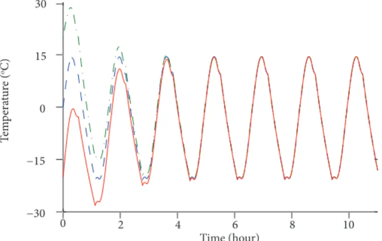
[(180° – ξ)/ω, (180° + ξ)/ω)], and [270°/ω, 360°/ω]. The intervals [nP, (n + 1)P], n = 1,2,..., were divided analogously. Using the solution computed at the end of a given subinterval as initial condition for the next subinterval, we prevent the differential equation solver from stepping across discontinuities. The solutions calculated for different initial temperatures are shown in Fig. 8. They approach the same periodic oscillation regardless of the initial value.

Figure 8. Predicted satellite temperature obtained from the numerical solution of Eq. 1 for different initial conditions.

0 2 4 6 8 10

−30 −15 0 15 30

Time (hour)

T

em

p

era

tur

e (

oC)

A checking criterion is available for the numerical solution: the long term mean value of T4₍_t_{) can be known without solving}

Eq. 1, as follows. Integrating Eq. 1 over one period gives (Eq. 25),

(25)

(26)

(27)

(28)

(29)

For n sufficiently large, T(t) has reached the asymptotic periodic behavior, T(nP) = T[(n + 1)P], and so the integral on the left-hand side of Eq. 25 vanishes, giving the relation (Eq. 26),

where we have used the periodicity of Q_tot(t) to change the limits of integration on the right-hand side. Defining the mean temperature T₀ as (Eq. 27),

from Eq. 26, we obtain (Eq. 28),

where Q₀ is the mean heat flux (Eq. 29), ×

ω ω ξ ω ξ ω ξ ω [(180° + 𝜉𝜉)/𝜔𝜔, 270°/𝜔𝜔]

ω ω

𝐶𝐶 q(éè8)ê𝑑𝑑𝜎𝜎_{𝑑𝑑𝑡𝑡 𝑑𝑑𝑡𝑡}

éê = −𝐴𝐴)**𝜎𝜎 q 𝜎𝜎

+_{𝑑𝑑𝑡𝑡} (éè8)ê

éê + q 𝑄𝑄./.(𝑡𝑡)𝑑𝑑𝑡𝑡

(éè8)ê

éê .

𝐴𝐴)**

𝜎𝜎 q

(éè8)ê

𝜎𝜎

+

_{𝑑𝑑𝑡𝑡}

éê

= q

𝑄𝑄./.(𝑡𝑡)𝑑𝑑𝑡𝑡

(éè8)ê

a

,

𝜎𝜎

a+

=

_𝑃𝑃

1 q

𝜎𝜎

+

(𝑡𝑡)𝑑𝑑𝑡𝑡

(éè8)ê

éê

,

𝜎𝜎

a+

=

_{𝐴𝐴)**𝜎𝜎}

𝑄𝑄a

=

1 _𝑃𝑃

q 𝑄𝑄

ê ./.(𝑡𝑡)𝑑𝑑𝑡𝑡

a

.

𝐴𝐴)**𝜎𝜎 q

(éè8)ê

𝜎𝜎

+

_{𝑑𝑑𝑡𝑡}

éê

= q

𝑄𝑄./.

(𝑡𝑡)𝑑𝑑𝑡𝑡

(éè8)ê

a

,

𝜎𝜎

a+

=

1 _𝑃𝑃

q

𝜎𝜎

+

(𝑡𝑡)𝑑𝑑𝑡𝑡

(éè8)ê

éê

,

𝜎𝜎

a+

=

_{𝐴𝐴)**𝜎𝜎}

𝑄𝑄a

=

1 _𝑃𝑃

q 𝑄𝑄./.(𝑡𝑡)𝑑𝑑𝑡𝑡

ê

a

.

𝐴𝐴)**

𝜎𝜎 q

(éè8)ê

𝜎𝜎

+

_{𝑑𝑑𝑡𝑡}

éê

= q

𝑄𝑄./.(𝑡𝑡)𝑑𝑑𝑡𝑡

(éè8)ê

a

,

𝜎𝜎

a+

=

_𝑃𝑃

1 q

𝜎𝜎

+

(𝑡𝑡)𝑑𝑑𝑡𝑡

(éè8)ê

éê

,

𝜎𝜎

a+

=

_{𝐴𝐴)**𝜎𝜎}

𝑄𝑄a

=

1 _𝑃𝑃

q 𝑄𝑄

ê ./.(𝑡𝑡)𝑑𝑑𝑡𝑡

a

.

𝐴𝐴)**𝜎𝜎 q

(éè8)ê

𝜎𝜎

+

_{𝑑𝑑𝑡𝑡}

éê

= q

𝑄𝑄./.(𝑡𝑡)𝑑𝑑𝑡𝑡

(éè8)ê

a

,

𝜎𝜎

a+

=

_𝑃𝑃

1 q

𝜎𝜎

+

(𝑡𝑡)𝑑𝑑𝑡𝑡

(éè8)ê

éê

,

𝜎𝜎

a+

=

_{𝐴𝐴)**𝜎𝜎}

𝑄𝑄a

=

_𝑃𝑃

1 q 𝑄𝑄./.(𝑡𝑡)𝑑𝑑𝑡𝑡

ê

(12)

xx/xx 12/24

We computed T₀ by two alternative ways: (i) applying the definition Eq. 26 to the numerically computed T(t) with n = 50; and (ii) using Eq. 27. The two T₀-values found agreed within the first six significant figures, T₀ = 270.210 K ≈ –2.9 °C, supporting the validity of the numerical solution.

Additional features of the solution T(t) can be understood through linearization of Eq. 1 around T₀. We define the deviation from T₀ as T*₍_t_{) =}_T₍_t_{) –}_T

0. Substituting T

*_{into Eq. 1, we have (Eq. 30)}

(30) (31) (32) (33) (34) (35) (36) (37) (38) (39)

where Q*₍_t_{) =}_Q

tot – Q0. Assuming |T

*_{| <<}_T

0 allows the use of the approximation (1 + T

*_/_T

0)

4_{≈ 1 + 4}_T*_/_T

0 which, together with

Eq. 28, turns Eq. 30 into its linearization (Eq. 31),

where the time constant τ is given by (Eq. 32),

To solve Eq. 30, we rely on the Fourier series expansion of Q*₍_t_{) (Eq. 33),}

where (Eq. 34),

Fig. 9a shows the approximation to Q_tot given by the three-term partial sum Q₂(t) = Q₀ + a₁ cos(ωt) + a₂ cos(2ωt). The steady state solution of Eq. 31 can be written as (Eq. 35),

where p_n(t) is the steady state solution of (Eq. 36),

given by (Eq. 37),

with (Eq. 38),

and (Eq. 39),

≈

𝐶𝐶𝑑𝑑𝜎𝜎_{𝑑𝑑𝑡𝑡 = −𝐴𝐴}∗ )**𝜎𝜎(𝜎𝜎a+ 𝜎𝜎∗)++ 𝑄𝑄a+ 𝑄𝑄∗(𝑡𝑡),

≪

≈

𝑑𝑑𝜎𝜎∗

𝑑𝑑𝑡𝑡 = −𝜎𝜎

∗

𝜏𝜏 +𝑄𝑄

∗_(𝑡𝑡)

𝐶𝐶 ,

τ

𝜏𝜏 =_4𝐴𝐴 𝐶𝐶

)**𝜎𝜎𝜎𝜎aZ≈ 65.2 min. ≈

≪

≈

𝑑𝑑𝜎𝜎∗

𝑑𝑑𝑡𝑡 = − 𝜎𝜎∗

𝜏𝜏 + 𝑄𝑄∗_(𝑡𝑡)

𝐶𝐶 ,

τ

)**𝜎𝜎𝜎𝜎aZ≈ 65.2 min. ≈

≪

≈

𝑑𝑑𝜎𝜎∗

𝑑𝑑𝑡𝑡 = −𝜎𝜎

∗

𝜏𝜏 +𝑄𝑄

∗_(𝑡𝑡)

𝐶𝐶 ,

τ

)**𝜎𝜎𝜎𝜎aZ≈ 65.2 min.

𝑄𝑄∗_{(𝑡𝑡) = 3 𝑎𝑎}

écos(𝑛𝑛𝜔𝜔𝑡𝑡), ñ

é78

𝑎𝑎é=_êk∫ 𝑄𝑄_aê ∗(𝑡𝑡) cos(𝑛𝑛𝜔𝜔𝑡𝑡)𝑑𝑑𝑡𝑡.

ω ω

𝜎𝜎∗_{(𝑡𝑡) = ∑} _𝑝𝑝 é(𝑡𝑡) ñ é78 ôöõ ô. = öõ ú + :õ ù cos(𝑛𝑛𝜔𝜔𝑡𝑡),

𝑝𝑝é(𝑡𝑡) = 𝒜𝒜écos(𝑛𝑛𝜔𝜔𝑡𝑡 − 𝜓𝜓é)

𝑄𝑄∗_{(𝑡𝑡) = 3 𝑎𝑎}

é78

𝑎𝑎é=_êk∫ 𝑄𝑄_aê ∗(𝑡𝑡) cos(𝑛𝑛𝜔𝜔𝑡𝑡)𝑑𝑑𝑡𝑡. (

ω ω

𝜎𝜎∗_{(𝑡𝑡) = ∑}ñ _𝑝𝑝_é_(𝑡𝑡) é78 ôöõ ô. = öõ ú + :õ ù cos(𝑛𝑛𝜔𝜔𝑡𝑡),

𝑄𝑄∗_{(𝑡𝑡) = 3 𝑎𝑎}

é78

ω ω

𝜎𝜎∗_{(𝑡𝑡) = ∑} _𝑝𝑝 é(𝑡𝑡) ñ é78 ôöõ ô. = öõ ú + :õ ù cos(𝑛𝑛𝜔𝜔𝑡𝑡),

𝑄𝑄∗_{(𝑡𝑡) = 3 𝑎𝑎}

é78

ω ω

𝑄𝑄∗_{(𝑡𝑡) = 3 𝑎𝑎}

é78

ω ω

𝒜𝒜é

=

𝑎𝑎é𝜏𝜏

𝐶𝐶†1 + (𝑛𝑛𝜏𝜏𝜔𝜔)

k

𝜓𝜓é

= tan

D8

_{( 𝑛𝑛𝜔𝜔𝜏𝜏)}

𝜎𝜎

k(𝑡𝑡) = 𝜎𝜎a

+ 𝒜𝒜8cos(𝜔𝜔𝑡𝑡 − 𝜓𝜓8) + 𝒜𝒜kcos(2𝜔𝜔𝑡𝑡 − 𝜓𝜓k

)

𝒜𝒜

8

1/𝑃𝑃 ∫ [𝜎𝜎k(𝑡𝑡) − 𝜎𝜎a]𝑑𝑑𝑡𝑡 = 0,

_aê

𝛿𝛿 = 1/𝑃𝑃 ∫ 𝜎𝜎

ê ∗

_{(𝑡𝑡)𝑑𝑑𝑡𝑡 < 0}

a

𝛿𝛿 = 𝜎𝜎£ − 𝜎𝜎

a

𝒜𝒜é

=

𝑎𝑎é𝜏𝜏

𝐶𝐶†1 + (𝑛𝑛𝜏𝜏𝜔𝜔)

k

𝜓𝜓é

= tan

D8

_{( 𝑛𝑛𝜔𝜔𝜏𝜏)}

𝜎𝜎

+ 𝒜𝒜8cos(𝜔𝜔𝑡𝑡 − 𝜓𝜓8) + 𝒜𝒜kcos(2𝜔𝜔𝑡𝑡 − 𝜓𝜓k

)

𝒜𝒜

8

1/𝑃𝑃 ∫ [𝜎𝜎k(𝑡𝑡) − 𝜎𝜎a]𝑑𝑑𝑡𝑡 = 0,

_aê

𝛿𝛿 = 1/𝑃𝑃 ∫ 𝜎𝜎

ê ∗

_{(𝑡𝑡)𝑑𝑑𝑡𝑡 < 0}

a

(13)

xx/xx 13/24

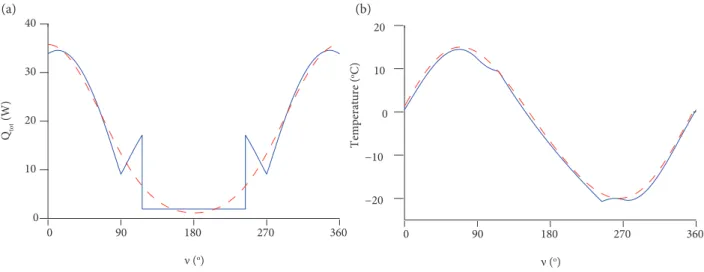
Figure 9b shows the approximation T₂(t) to the solution T(t) given by the first three Fourier modes, . Note how T₂(t) is able to capture the amplitude of the oscillations. The analysis based on linearization, here shown, although approximate, has the advantage of providing simple relations (Eqs. 28, 32 and 38) between the model parameters and attributes of the solution. To appreciate the usefulness of Eq. 38, the reader is invited to reckon a₁ from visual inspection of Fig. 9a, substitute the approximate a₁-value on Eq. 38, and compare the temperature oscillation amplitude so calculated with the actual one shown in Fig. 9b.

Figure 9. (a) Total external heat flux Q_tot (solid line) and three-term partial sum of the Fourier series expansion of Q_tot, Q₂(t) = Q₀ + a₁ cos(v) + a₂ cos(2v) (dashed line). (b) Numerically computed asymptotic periodic temperature T(t) (solid line)

and three-Fourier-mode approximation T2(t) = T0 + A1cos (ωt – ψ1) + A2cos (2ωt – ψ1)(dashed line). 0

10 20 30 40

Qtot

(W)

Temperature (

oC)

−20 −10 0 10 20

0 90 180

ν (o₎

270 360 0 90 180

ν (o₎

270 360

We end this section explaining a detail of Fig. 9b: T₂(t) is slightly above T(t). This is due to T₂(t) – T₀ and T*₍_t_{) having different} time-averages. 1/P ∫ P ₀ [T₂(t) – T₀ ]dt = 0, while δ = 1/P ∫ P ₀T*₍_t₎_dt_{< 0. To see this, integrate}_T*₍_t_{) =}_T₍_t_{) –}_T

0 over one period to

obtain (Eq. 40),

where T – = 1/P ∫ P ₀T*₍_t₎_dt_{. Jensen’s inequality (Rudin 1970) implies that, for non-constant}_T₍_t_),_T–_<_T

0. Hence, δ < 0.

YEARLY VARIATION OF THE RADIATION SCENARIO

In this section, we discuss important changes in the solar and albedo heat fluxes that take place over a time scale of several months for general satellite orbits. They are the result of variations in the angle between the satellite orbital plane and the solar vector ŝ (the minimum of the angles between all orbital positions r_sat and ŝ), known as the β angle. To see how β affects the solar heat flux Q_S falling on the satellite, contrast the time-periodic Q_S found for the orbit in the previous section (β = 0°) to the time-constant Q_S expected for velocity-nadir attitude and a circular orbit on a plane perpendicular to ŝ (β = 90°). The orientation of the orbital plane is given by the normal vector ˆl computed as the direction of the orbital angular momentum l = r_sat × v_sat, with v_sat the satellite velocity, l ˆ = l/||l||. Moreover, from the definition of β, we have (Eq. 41)

(40)

(41)

During the year, both l ˆ and ŝ rotate with respect to the GECS. We will express both vectors on the {û₁, û₂, û₃} basis, and, using Eq. 41, obtain β. But first, we introduce the standard way of presenting a general spacecraft orbit.

𝒜𝒜é

=

𝑎𝑎

é

𝜏𝜏

𝐶𝐶†1 + (𝑛𝑛𝜏𝜏𝜔𝜔)

k

𝜓𝜓é

= tan

D8

_{( 𝑛𝑛𝜔𝜔𝜏𝜏)}

𝜎𝜎

+ 𝒜𝒜8cos(𝜔𝜔𝑡𝑡 − 𝜓𝜓8) + 𝒜𝒜kcos(2𝜔𝜔𝑡𝑡 − 𝜓𝜓k

)

𝒜𝒜8

1/𝑃𝑃 ∫ [𝜎𝜎k(𝑡𝑡) − 𝜎𝜎a]𝑑𝑑𝑡𝑡 = 0,

_aê

𝛿𝛿 = 1/𝑃𝑃 ∫ 𝜎𝜎

ê ∗

_{(𝑡𝑡)𝑑𝑑𝑡𝑡 < 0}

a

𝛿𝛿 = 𝜎𝜎£ − 𝜎𝜎a

𝜎𝜎£ = 1/𝑃𝑃 ∫ 𝜎𝜎(𝑡𝑡)𝑑𝑑𝑡𝑡_aê

𝜎𝜎£ < 𝜎𝜎a δ

𝜎𝜎k(𝑡𝑡) = 𝜎𝜎a+ 𝒜𝒜8cos(𝜔𝜔𝑡𝑡 − 𝜓𝜓8) + 𝒜𝒜kcos(2𝜔𝜔𝑡𝑡 − 𝜓𝜓k)

ŝ

ŝ β

β

ŝ β

𝒍𝒍•,

× 𝒍𝒍•

β

cos(90° − 𝛽𝛽) = 𝒔𝒔T ∙ 𝒍𝒍•

(14)

xx/xx 14/24

KEPLERIAN ORBITAL ELEMENTS

On a first approximation, the satellite orbit is described by a solution of Kepler problem (Vallado 1997), namely, an ellipse with one of its foci at the origin of the GECS. The orbit shape is described by the semimajor axis a and the eccentricity e = c/a, where c is half the distance between the foci. As e → 0, the ellipse approaches a circle (e = 0).

l ˆ is determined by the inclination i and the right ascension of the ascending node (RAAN) Ω through (Eq. 42) (see Fig. 10),

The ascending node is the orbital point on the equatorial plane at which the satellite moves from south to north. The orientation of the semimajor axis within the orbital plane is given by the argument of perigee g, defined as the angle between the position vectors of the ascending node and the periapsis, the location at which the satellite is closest to the origin (Fig. 10). Finally, the satellite position on the ellipse is set by the true anomaly v, measured from the periapsis. The Keplerian orbital elements a, , Ω, i,

g, and v completely specify a solution of Kepler problem (Vallado 1997; Bate et al. 1971).

(42)

ˆ l

Ω

i

g

Satellite

v û₃

û₁ Υ

û₂

ν

Periapsis

Ascending node Equatorial

plane

The orbital elements of Libertad 1 are available online from Space-Track (a service of the United States Department of Defense (JFCCS 2015)) in the two line element set (TLE) format. Elements , Ω, i, and g can be retrieved straightforwardly from a TLE. On the other hand, a needs to be computed from the mean motion (mean angular velocity) using Eq. 9 with R substituted by a. Similarly, ν is obtained from the mean anomaly (Vallado 1997).

Table 3 shows the orbital elements of Libertad 1 on April 18, 2007, 21 h 54 min 52.4 s Coordinated Universal Time (according to Portilla (2012), the orbital elements of Libertad 1 disclosed for prior times are possibly inaccurate). Note the low value of the eccentricity, which justifies our assumption of a circular orbit for Libertad 2. Observe also the closeness between a and the value of R assumed in the previous section.

The orbital elements of a spacecraft on a LEO do not stay constant. Of relevance to the thermal analysis is the change of the RAAN Ω, known as nodal regression and determined next.

Table 3. Orbital elements of satellite Libertad 1 on April 18, 2007, 21 h 54 min 52.4 s (JFCCS 2015). a: semi-major axis; e: eccentricity; v: true anomaly; i: inclination; Ω: Right Ascension of the Ascending Node (RAAN); g: argument of perigee (see Fig. 10).

a (km) e i (°) Ω (°) g (°) v(°)

7097.87 0.0102 98.08 184.09 207.97 154.07

Figure 10. Four of the six Keplerian orbital elements. i: inclination;

Ω: right ascension of the ascending node; g: argument of perigee; and v: true anomaly.

𝒍𝒍• ŝ

β

𝑒𝑒

𝑒𝑒 → 0 𝑒𝑒

𝒍𝒍•

Ω

𝒍𝒍• = sin 𝑖𝑖 sin Ω 𝒖𝒖N8− sin 𝑖𝑖 cos Ω 𝒖𝒖Nk+ cos 𝑖𝑖 𝒖𝒖NZ.

(15)

xx/xx 15/24

NODAL REGRESSION

The assumptions of Kepler problem are satisfied only when the planet has a perfectly spherical mass distribution. In actual fact, Earth presents a protrusion around the Equator, which can be thought of as a ring added to a sphere. This ring applies a gravitational torque that rotates the satellite orbital angular momentum, causing a drift of Ω (Fortescue et al. 2003) (Eq. 43),

û1

û₃

Υ

û₂

Ωs

δ

s

Sun

λ_ecl

E

Ecliptic Celestial Equator

sˆ

with a constant rate of nodal regression Ω .. . The protrusion is measured by the coefficient J₂ = 1.0826 × 10–3_{of the expansion in}

spherical harmonics of the gravitational potential generated by Earth (Fortescue et al. 2003; Vallado 1997). J₂ determines the rate of nodal regression through the relation (Fortescue et al. 2003; Vallado 1997) (Eq. 44),

(43)

(44)

(45)

where terms O (J 2

2) were neglected and a circular orbit of radius R and angular velocity ω, given by Eq. 9, was assumed.

VARIATION OF THE SOLAR VECTOR S ˆ AND OF

β

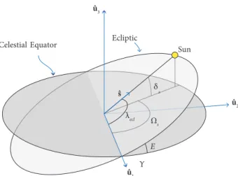
For a satellite on a LEO, the solar vector ŝ is essentially the unit vector in the direction of the Sun’s position with respect to the GECS. Due to the tilt of the Earth’s rotational axis relative to the plane of its orbit, from the geocentric point of view, the Sun traverses an orbit on a plane (the ecliptic) inclined roughly 23° with respect to the Equatorial plane (Fig. 11). In fact, by definition, the û₁ vector points toward the ascending node of the Sun’s orbit, or point of Aries () (Fig. 11). ŝ is determined by the Sun’s longitude Ω_S and declination δ_S with respect to the GECS (Fig. 11) (Eq. 45),

The evolution of Ω_S and δ_S can be computed by algorithms available in Vallado (1997), Nautical Almanac Office (2008), and Fitzpatrick (2010) or it can be obtained from online resources (Jubier 2004), such as NASA’s HORIZONS system (JPL 2015a). To produce an initial β angle similar to that of Libertad 1, we assume Libertad 2 will be deployed into orbit on April 19, 2019 at 0 h 0 min 0 s UTC. Figure 12 shows Ω_S and δ_S from the time of insertion into orbit, computed using the algorithm in Fitzpatrick (2010) (presented in Appendix A). Our values agree with HORIZONS apparent ephemeris within 0.01°.

Figure 11. Solar orbit on the Ecliptic in relation to the GECS. The figure also depicts the obliquity of the Ecliptic E, the ecliptic longitude of the Sun λ_ecl, the Sun’s longitude Ω_S, and the Sun’s declination δ_S.

Ω

Ω = Ωa− Ω̇𝑡𝑡

Ω̇

×

Ω̇ =3₂𝐽𝐽k_𝑅𝑅𝑅𝑅_k=k𝜔𝜔 cos 𝑖𝑖

𝑂𝑂(𝐽𝐽kk) ω

𝒔𝒔T 𝜷𝜷

ŝ

^ ŝ Ω

δ

Ω

Ω = Ωa− Ω̇𝑡𝑡