J. Aerosp. Technol. Manag., São José dos Campos, v10, e3718, 2018 1.Universidade de São Paulo – Escola de Engenharia de São Carlos – Departamento de Engenharia Aeronáutica – São Carlos/SP – Brazil.
Correspondence author: Marlon Sproesser Mathias | Universidade de São Paulo – Escola de Engenharia de São Carlos – Departamento de Engenharia Aeronáutica | Av. João Dagnone, 1100 | CEP: 13.566-590 – São Carlos/SP – Brazil | E-mail: [email protected]
Received: Feb. 27, 2017 | Accepted: Nov. 5, 2017
Section Editor: João Azevedo
ABSTRACT: This study takes a Jacobian-free approach based on the Arnoldi iteration to present a method to perform hydrodynamic instability analysis based on Direct Numerical Simulations. The method employs high order spatial and temporal discretizations for the flow simulation and has very low requirements of computational time and memory, compared to conventional matrix-forming methods. Details of the numerical treatment applied to guarantee consistency in the numerical solution are discussed, such as mesh and domain dependencies, and buffer zones for the open boundary conditions. The implementation presented here is applicable to any flow with Cartesian geometry, however, the method can be extended to complex geometries and three-dimensional flows.
KEYWORDS: Open cavity flow, Direct Numerical Simulation, Hydrodynamic instability, Compressible flow, Arnoldi iteration.
INTRODUCTION
An open cavity can be used to represent several different parts of an aircraft in flight, for example the gap between the slats or flaps and the main element of the wing, both at deployed and retracted positions. Better understanding of the flow mechanics over this simplified geometry can aid aircraft designers to predict the transition from laminar to turbulent flow over the wing and the slat’s influence over the flow instability, as well as the related acoustic emissions (Colonius 2001).
This paper shows the development of a DNS for this flow. Special attention is given to the high order spatial and temporal discretizations applied to instability and acoustic analysis. For spatial discretizations, various numerical schemes were employed in the DNS, including compact finite differences with spectral-like resolution (Lele 1992). These schemes allow the code to resolve a wider range of scales than traditional finite difference schemes. Time integration was performed with a standard fourth-order Runge Kutta method.
Depending on the Reynolds and Mach numbers, and cavity aspect ratio, the flow can reach a stationary or a periodic state; Brès and Colonius (2008) bring a diagram showing this fact for a fixed cavity aspect ratio. By increasing the Reynolds number, three-dimensional instabilities are observed at lower Mach numbers, while two-three-dimensional instabilities tend to be triggered first if the Mach number is higher. For a length to depth ratio of 2, flows above a ReD of roughly 1300 are 3D unstable, this value is normalized by the cavity depth, D. The minimum Re for a 2D unstable flow is reduced as the Mach number increases, becoming lower than the 3D instability threshold around Mach 0.4. These instabilities eventually saturate to become periodic oscillations in the flow.
Direct Numerical Simulation of a
Compressible Flow and Matrix-Free Analysis
of its Instabilities over an Open Cavity
Marlon Sproesser Mathias1, Marcello Medeiros1
Mathias MS; Medeiros M (2018) Direct Numerical Simulation of a Compressible Flow and Matrix-Free Analysis of its Instabilities over an Open Cavity. J Aerosp Technol Manag, 10: e3718. doi: 10.5028/jatm.v10.949.
How to cite
Mathias MS https://orcid.org/0000-0002-2415-5723
J. Aerosp. Technol. Manag., São José dos Campos, v10, e3718, 2018 Mathias MS; Medeiros M
xx/xx 02/13
This DNS is used in conjunction with matrix-free instability analysis methods to compute the eigenvalues of the flow and their respective eigenfunctions. Regular matrix-forming methods would demand an enormous amount of memory to compute the flow modes, in the order of the squared total number of nodes in the domain multiplied by the number of variables, which would easily scale into terabytes of memory solely to store the required matrices (Theofilis 2011). This matrix-free method is based on the work of Eriksson and Rizzi (1985), who have implemented a method based on Arnoldi (1951) to find the most unstable or least stable modes of an inviscid flow around an airfoil.
Later works have applied the same methods on the full Navier-Stokes equations (Chiba 1998; Tezuka and Suzuki 2006) and also included shift-invert strategies to focus on eigenvalues in a specific region of the complex plane (Gómez Carrasco
et al. 2015).
This work extends this method to account for the compressibility, which is required for non-zero Mach numbers and for acoustic analysis. The code was developed for medium to high subsonic flows, which are commonly found in modern aircrafts.
METHODS
DIRECT NUMERICAL SIMULATION
The DNS code was developed by our group for several kinds of problems on hydrodynamic instability and aeroacoustics and was adapted for the open cavity flow (Martínez and Medeiros 2016). It is written in Fortran 90 and, for parallelization, uses both OpenMP and a domain decomposition technique with the 2decomp&fft library (Li and Laizet 2010), which uses MPI. The code uses a structured mesh in a rectangular domain. The grid is much finer in the cavity and close to the flat plate in the wall-normal direction. There is also a lower level of stretching in the stream-wise direction, concentrating nodes on the cavity, and making sure there are nodes positioned exactly on the cavity edges. Closer to the open boundaries, in both directions, the spacing is greatly increased, as part of a buffer zone. No multidomain technique is used in this case, grid points inside the wall are ignored by the solver. Figure 1 illustrates the domain, the buffer zone is shown in blue, while points inside the wall are orange, darker gray levels represent a finer grid.
Both the flat plate and the cavity walls have no-slip and no-penetration boundary conditions, as well as zero pressure gradient in the normal direction and constant temperature. Just upstream of the flat plate, there is a free-slip region to represent free flow before the leading edge of the no-slip wall, which allows the pressure gradients just before the boundary layer to be computed correctly.
The inflow boundary is defined as a uniform flow at constant temperature and zero stream-wise pressure gradient. At the outflow, pressure is kept constant and velocity is extrapolated by imposing the second derivative equal to zero.
The two top corners in the cavity were points of special attention for the boundary conditions. The Neumann condition for pressure in other points is observed by computing the density in each node of the boundary so that the derivative of the pressure is null in the normal direction at the wall. Both corner nodes present a problem as walls in distinct directions meet and the density that observes the Neumann condition in one direction might violate it for the other. The pressure in both these nodes is set to the mean of the pressures that meet the boundary condition for each direction.
At the open boundaries of the domain, a special treatment must be done so oscillations are neither reflected nor amplified. Buffer zones were put in place, they are a non-physical region designed to avoid these issues. In these work, the following techniques were used:
• Increased node spacing compared to the regular mesh • Decreased spatial derivative order
• A Selective Frequency Damping low-pass filter (Åkervik et al. 2006)
There is a smooth transition from the physical domain to the buffer zone to avoid issues at the interface.
J. Aerosp. Technol. Manag., São José dos Campos, v10, e3718, 2018
At the buffer zone, the scheme is smoothly replaced by a second-order explicit one, with a much lower spectral accuracy. The transition is handled by a cosine function, which multiplies the finite differences coefficients (Eq. 1):
Figure 1. Illustration of the domain and its boundaries. Buffer zone is shown in blue, points inside the
wall are orange, darker grays indicate a finer grid.
Open boundary
Buffer zone
B
uff
er zo
ne
B
uff
er zo
ne
Ou
tfl
o
w
In
fl
ow
Wall Wall
Free-slip
Wall
where: a is the coefficient actually used by the solver; aH and aL are the high-order and low-order coefficients, respectively; η is zero at the physical domain and is linearly increased to one at the end of the buffer zone. The process is repeated for all finite differences coefficients.
Once more, both the corner nodes presented a challenge for these methods when computing the derivative. Figure 2 illustrates the Regions considered. In an inner node, i.e. one away from the boundaries, finite differences method uses the nodes around it to approximate the derivative. If no other changes were made to the code, corners nodes 1 and 2 would be considered as inner nodes and, thus, derivatives computed for them would account for both points on the wall and points immersed in the flow, which would not be correct and cause the solution to fail. Because of this, both nodes only consider values in Region 2 of Fig. 2.
𝑎𝑎 = cos(𝜋𝜋 𝜂𝜂) 𝑎𝑎
++ (1 − cos(𝜋𝜋 𝜂𝜂)) 𝑎𝑎
/η
(1)
Figure 2. Close-up of the corner nodes in the domain and the Regions considered for derivatives.
This has solved the problem for both corner nodes and for the Region between them. But nodes in Regions 1 and 3 of the figure would still have its derivatives miscalculated, causing discontinuities in the domain close to the corner, which would later cause the simulation to fail. This was solved by considering both the last node in Region 1 and the first node in Region 3 as inner nodes for the finite differences method, which makes the derivative a continuous function again.
In sum, derivatives in Region 2 depend only on values in it. Derivatives in Regions 1 and 3 depend on values both in their respective region and on values in Region 2. The approach for wall-normal derivatives is analogous.
Equation 2 illustrates how the derivatives would be computed close to corner node 1, with index c_1. α, a, b, and c are the finite differences coefficients, note that they are different for the corner nodes and more coefficients may be added depending on the chosen derivative scheme. D and f are vectors containing the derivatives and the function values for each node, respectively.
Region 1
Corner node 1 Corner node 2
Cavity
Region 2 Region 3
J. Aerosp. Technol. Manag., São José dos Campos, v10, e3718, 2018 Mathias MS; Medeiros M
xx/xx 04/13
Time integration is performed at a fixed time step by either an explicit Euler, a second order or a fourth order Runge-Kutta scheme. As default, the fourth-order scheme is used.
The initial condition is defined as free-flow velocity above the flat plate and zero velocity in the cavity, at constant pressure and temperatures. Results from previous runs can also be used as initial condition as long as they share the same mesh. Reynolds and Mach numbers and the numerical methods may be changed.
All values are non-dimensional, being normalized by the free flow stream-wise velocity, cavity depth and initial density, the base time is given by the base length divided by the base length (Martínez 2016).
In this type of simulation, high-frequency numerical noise may quickly build up, causing the simulation to diverge from the physical solution. To attenuate this noise, numerical low-pass filters are implemented (Gaitonde and Visbal 1998). The filter strength can be adjusted before runtime and, ideally, should be as low as possible, minimizing its effect on results. Filtering is turned off a few nodes away from the boundary due to the large derivatives present and to avoid using uncentered stencils.
The implementation described here was done for a two-dimensional domain, which assumes all variables as constant in the span-wise direction. This is a valid assumption for stability analysis as long as the flow conditions are such that two-dimensional modes become unstable before three-dimensional ones.
MATRIX-FREE INSTABILITY ANALYSIS
In order to find the oscillation modes of a certain system, one has to compute the eigenvalues and eigenvectors of the flow Jacobian matrix. It is, given that the Navier-Stokes equations and all boundary conditions are described by (Eq. 3)
α
⎣
⎢
⎢
⎢
⎢
⎢
⎡ 1 𝛼𝛼
𝛼𝛼
1 𝛼𝛼
⋯ 0
⋮
⋱ ⋱ ⋱
𝛼𝛼 1 𝛼𝛼
1 𝛼𝛼
⋮
𝛼𝛼 1 𝛼𝛼
0 ⋯
⋱ ⋱ ⋱ ⎦
⎥
⎥
⎥
⎥
⎥
⎤
⎣
⎢
⎢
⎢
⎢
⎢
⎡
𝐷𝐷
𝐷𝐷
<=
⋮
𝐷𝐷
>?@<𝐷𝐷
>?𝐷𝐷
>?A<⋮
⎦
⎥
⎥
⎥
⎥
⎥
⎤
=
⎣
⎢
⎢
⎢
⎢
⎢
⎡ 𝑎𝑎
−𝑎𝑎 0
𝑏𝑏
𝑎𝑎
𝑐𝑐
⋯ 0
⋮
⋱
⋱
⋱
−𝑎𝑎 0
𝑎𝑎
𝑎𝑎
𝑏𝑏
𝑐𝑐
⋮
−𝑎𝑎 0 𝑎𝑎
0
⋯
⋱ ⋱ ⋱ ⎦
⎥
⎥
⎥
⎥
⎥
⎤
⎣
⎢
⎢
⎢
⎢
⎢
⎡
𝑓𝑓
𝑓𝑓
<=
⋮
𝑓𝑓
>?@<𝑓𝑓
>?𝑓𝑓
>?A<⋮
⎦
⎥
⎥
⎥
⎥
⎥
⎤
α
⎣
⎢
⎢
⎢
⎢
⎢
⎡ 1 𝛼𝛼
𝛼𝛼
1 𝛼𝛼
⋯ 0
⋮
⋱ ⋱ ⋱
𝛼𝛼 1 𝛼𝛼
1 𝛼𝛼
⋮
𝛼𝛼 1 𝛼𝛼
0 ⋯
⋱ ⋱ ⋱ ⎦
⎥
⎥
⎥
⎥
⎥
⎤
⎣
⎢
⎢
⎢
⎢
⎢
⎡
𝐷𝐷
𝐷𝐷
<=⋮
𝐷𝐷
>?@<𝐷𝐷
>?𝐷𝐷
>?A<⋮
⎦
⎥
⎥
⎥
⎥
⎥
⎤
=
⎣
⎢
⎢
⎢
⎢
⎢
⎡ 𝑎𝑎
−𝑎𝑎 0
𝑏𝑏
𝑎𝑎
𝑐𝑐
⋯ 0
⋮
⋱
⋱
⋱
−𝑎𝑎 0
𝑎𝑎
𝑎𝑎
𝑏𝑏
𝑐𝑐
⋮
−𝑎𝑎 0 𝑎𝑎
0
⋯
⋱ ⋱ ⋱ ⎦
⎥
⎥
⎥
⎥
⎥
⎤
⎣
⎢
⎢
⎢
⎢
⎢
⎡
𝑓𝑓
𝑓𝑓
<=
⋮
𝑓𝑓
>?@<𝑓𝑓
>?𝑓𝑓
>?A<⋮
⎦
⎥
⎥
⎥
⎥
⎥
⎤
(2) (3) (4) EFEG
= 𝑓𝑓(𝑢𝑢)
𝐴𝐴 =
EJ(F)EF(
×
×
×
×
where u is a vector that contains all flow variables for each node in the mesh, the Jacobian is given by Eq. 4
The size of this matrix is 4N × 4N for two-dimensional flows and 5N × 5N for three-dimensional. Four and five are the numbers of variables for each node, respectively, and N is the number of nodes in the domain. Given the domain’s size is usually in the order of hundreds of points in the stream-wise and wall-normal directions and a few dozens of points in the span-wise direction, the total number of variables to solve for is in the order of 105 to 106 in two-dimensional cases, and 106 to 107 when accounting for the third dimension.
J. Aerosp. Technol. Manag., São José dos Campos, v10, e3718, 2018
The method used in this work was proposed by Eriksson and Rizzi (1985) for the Euler equations and first implemented by Chiba (1998) for the incompressible Navier-Stokes equations. It is based on Arnoldi’s method for solving the eigenproblem.
The most important feature of the method is to be able to approximate the most unstable or least stable modes without storing the Jacobian matrix for the flow. The DNS itself is embedded into the method instead of being linearized to the Jacobian matrix. In summary, the method adds small disturbances to the steady-state flow and uses the DNS to observe how the flow reacts to them, as will be described below. After a series of orthogonal disturbances, the Hessenberg matrix from the Arnoldi (1951) method is obtained, which is several orders of magnitude smaller than the flow’s Jacobian matrix would be. The eigenvalues and eigenvectors of this matrix are computed and, finally, used to approximate the flow’s modes and their respective amplification or attenuation rates. This is shown in the flowchart in Fig. 3.
Figure 3. Flowchart of matrix-free method for computing the flow modes.
(1) Steady state flow U
0
U
0
from DNS
(2) Initial disturbance ζ k
ζ k
of norm 1 with k = 1
(3) Compute flows Uk+ U
Uk+
Uk+
k
and −
U k −
Uk−
by adding and
subtracting ε from , respectively
(4) Run DNS from and for t time, resulting
flows are ˜
U˜k+
and ˜
U
k
− ˜
, respectively
(5) Bζ
k
Bζ
k
= ( − ) / 2ε
(6) h
j,k = ζ T j ·Bζk
k
j
j = 1
= 1 ...k
(7) ˜u
k+1
k+1
k+1
k+1
k+1
= −
Σ
hj,k ζj
(8) h ,k
k+1
h ,k
= || ˜u ||
(9) ζ = ˜u
(10) k = k + 1, repeat while k ≤ M
(11) Compute eigenvalues σ H and eigenvectors φ H
φ H
of H
(12) σ A= log (σ H )/t
/
and φ A = { ζ 1 . . . ζk}
Steps (6) to (11) from Fig. 3 are taken directly from the Arnoldi iteration method.
Eriksson and Rizzi (1985) use a random vector for the initial disturbance at step (2). Chiba (1998) computes it as a random vorticity field, for which the Poisson equation is solved numerically, resulting in the disturbance’s stream function. In this work, a Gaussian disturbance to all variables, centered close to the cavity, is used.
In step (3) of Fig. 3, ε controls the norm of the perturbation; it is worth noting that the number of mesh nodes influences the module of the perturbation in each node. This variable should be adjusted so that the perturbation is small enough to non-linearities remain small, but should be large enough so numerical and roundoff errors influence on results are also small.
J. Aerosp. Technol. Manag., São José dos Campos, v10, e3718, 2018 Mathias MS; Medeiros M
xx/xx 06/13
In step (5), a second-order central finite differences scheme is used, Eriksson and Rizzi note that higher order methods may be used, this reduces the effect of non-linearities in the results but requires more DNS runs.
It should also be noted that in step (12), the equation for eigenvalues is not fully reversible for the imaginary part, as the exponential function of a complex number is not injective. This means that the method brings a correct approximation only for the real part of the eigenvalues, related to the amplification rate. The imaginary part, related to the frequency, may have a factor of n × 2 π/t added to it, where n is any integer. It must be checked by other means, for example by using the DNS to simulate each one of the modes identified and observing the oscillation frequencies.
Shift-invert strategies may also be used in conjunction with this method, as done by Gómez Carrasco et al. (2015). This allows Arnoldi’s method to retrieve modes in a specific Region of the complex plane, for example, it could obtain modes related to acoustic of the flow, which may be more stable than other modes.
A code for this routine was implemented in Matlab, it calls the Fortran DNS as necessary. An important perk of this method is that it can be programmed in a very modular way. The DNS could be easily replaced or updated with only minor changes to the Matlab code. All parallel processing capabilities of the DNS are retained and another one is added, as both positive and negative disturbance cases can be ran simultaneously by concurrent processes.
RESULTS
The validation of the method shown in this section is divided in three parts. First, the DNS is validated by comparing its results to previous ones by Colonius et al. (1999). After that, the method is checked against itself by changing parameters such as the mesh, domain, number of iterations and so on, making sure the results are well converged with respect to them. Later, its results are compared to the Residual Algorithm, as described by Theofilis (2000; 2003) and Gómez et al. (2012).
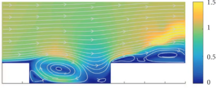
For the DNS validation, a case described by Colonius et al. (1999) was selected. The Reynolds number with respect to the cavity depth is ReD = 1530, Mach number is Ma = 0.6, and the cavity aspect ratio is L/D = 4. This represents an unstable flow, which should evolve in time until reaching a periodic state. Figure 4 illustrates this flow at an arbitrary time after becoming periodic.
Figure 4. Velocity magnitude and streamlines of the unsteady flow at an arbitrary time.
Two meshes, described in Table 1, were used for this analysis.
Table 1. Meshes used for convergence analysis.
Mesh 1 Mesh 2
Nodes in x 300 400
Nodes in y 150 200
Nodes in x (inside cavity) 144 192
Nodes in y (inside cavity) 52 70
1.5
1
0.5
J. Aerosp. Technol. Manag., São José dos Campos, v10, e3718, 2018
Figure 5 shows the wall-normal velocity plotted against time at a fixed point at the flat plate height, three quarters across the opening.
Figure 5. Velocity plotted against time at a fixed point in an unsteady case.
A case described by de Vicente et al. (2014) was used as base for the instability analysis. In this case, the cavity’s aspect ratio is L/D = 2, the Reynolds number is ReD = 1149, and the boundary layer thickness at the cavity’s leading edge is θ = 0.0337. All lengths are normalized by the cavity depth and all velocities, by the inflow velocity.
The reference case has assumed the flow as incompressible. To approximate this assumption, the Mach number was set as Ma = 0.1. Low Mach numbers require a shorter time step to maintain numerical stability, considerably increases the computational cost. MESH AND DOMAIN CONVERGENCE
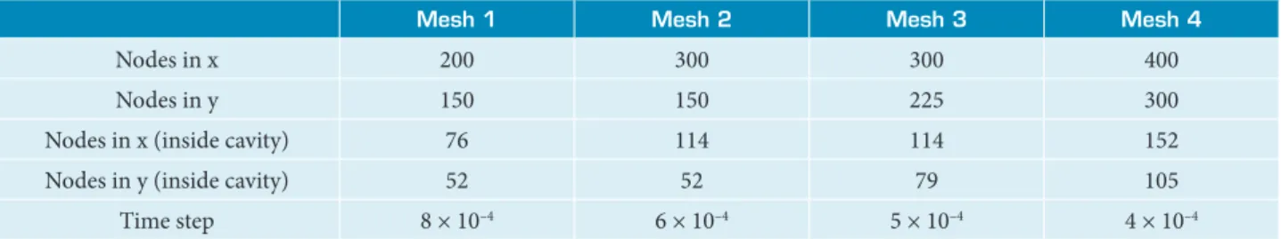
Four meshes, shown in Table 2, were used in the mesh convergence analysis.
Table 2. Meshes used for convergence analysis.
Mesh 1 Mesh 2 Mesh 3 Mesh 4
Nodes in x 200 300 300 400
Nodes in y 150 150 225 300
Nodes in x (inside cavity) 76 114 114 152
Nodes in y (inside cavity) 52 52 79 105
Time step 8 × 10⁻⁴ 6 × 10⁻⁴ 5 × 10⁻⁴ 4 × 10⁻⁴
All these meshes are for the same domain, which spans from xi = –2 to xf = 10 and from yi = –1 to yf = 4. The cavity is placed from x1 = 2.9597 to x2 = 4.9597, and from y1 = 0 to y2 = –1. They also share the same parameters for the buffer zones, which add 20 nodes in each direction.
Note that the time step was reduced, as the mesh got finer so that the numerical stability was ensured. The CFL number was always kept close to 1.
The disturbance magnitude parameter ε0 was set to 10–5. It was used 400 Arnoldi iterations for each case. Convergence tests for these parameters are shown later in this work. The number of steps at each iteration was adjusted so that the physical run time was the same, for meshes 1 to 4 it was set to 500, 667, 800 and 1000, respectively.
Figure 6 shows the eigenvalues retrieved for these meshes. The right-hand side image depicts the least stable modes in detail. The real part of the eigenvalue relates to the mode’s stability. Positive values are unstable and negative values are stable. Its imaginary part relates to the mode’s frequency. If any of the modes has a positive real part, the whole flow is considered unstable.
Time
-0.5 0
0 5 10 15 20 25 30 35
0.5 1
Velocity
J. Aerosp. Technol. Manag., São José dos Campos, v10, e3718, 2018 Mathias MS; Medeiros M
xx/xx 02/13
All four meshes have resulted in similar values for the 12 least stable modes.
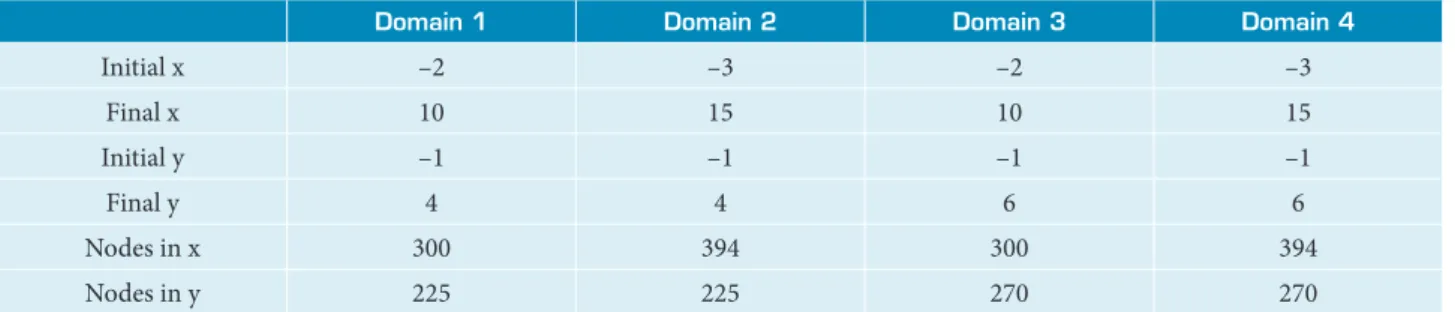
A similar analysis was ran for the domain size. Table 2 shows the values used. Mesh 2 from Table 2 was used as Domain 1 for this analysis. The increase in the total number of nodes was needed so that the refinement at the cavity was constant.
Table 3. Domains used for convergence analysis.
Domain 1 Domain 2 Domain 3 Domain 4
Initial x –2 –3 –2 –3
Final x 10 15 10 15
Initial y –1 –1 –1 –1
Final y 4 4 6 6
Nodes in x 300 394 300 394
Nodes in y 225 225 270 270
The eight least stable modes from all domains have matching eigenfunctions, as can be seen in Fig. 7. Mode 9 of Domains 2, 3 and 4 matches the eigenfunction of mode 11 of the smaller domain, leading to the conclusion that it is the same mode, both its eigenvalue was miscalculated.
Figure 6. Eigenvalues in the complex plane for various meshes.
Figure 7. Eigenvalues in the complex plane for various domains.
Another run was performed with 600 Arnoldi iterations instead of 400. At this time, all domains match up to the 15th mode, leading to the conclusion that the bottleneck in this case was more than just the domain size.
-8 -6 -4 -2
-1 –0.5 0
0
σ
r σr
-0.2 –0.1 0
σi
σi
2 4 6 8
-2 -1.5 -1 -0.5 0 0.5 1 1.5 2
Mesh 1 Mesh 2 Mesh 3 Mesh 4
-8 -6 -4 -2
-1 –0.5 0
0
σ
r
-0.2 –0.1 0
σ
r
σi
σi
2 4 6 8
-2 -1.5
-1 -0.5
0 0.5 1 1.5 2
J. Aerosp. Technol. Manag., São José dos Campos, v10, e3718, 2018
ARNOLDI ITERATION CONVERGENCE
In this section, the parameters relative to the instability analysis method are checked. Three items are considered: the number of Arnoldi iterations (M); the number of DNS time steps at each Arnoldi iteration (nT); and the magnitude of the disturbance added to the baseflow (ε0). Mesh 2 of Table 1 is used as base.
Figure 8 shows the evolution of the 15 least stable eigenvalues as the Arnoldi method is iterated, both the real and imaginary parts. The issue seen at the domain convergence analysis can be understood more clearly here, note that the last eigenvalues are not yet converged after 400 iterations.
Figure 8. Eigenvalues computed after each Arnoldi iteration.
A convergence analysis was also performed for the number of time steps the DNS is run each time it is called. Figure 9 shows the complex plane for various numbers of time steps. The nT = 200 case is not converged, as it has resulted in a different set of eigenvalues. The nT = 400 case diverges at the third mode. The other two results match, usually up to the eighth decimal place for the first few eigenvalues. From the mode 13 and onwards, the nT = 667 case also starts diverging.
Figure 9. Effect of the number of time steps on the eigenvalues retrieved.
It is worth noting how the range of values for σi reduces as the number of steps is increased. This is due to the last equation in the flowchart of Fig. 5. This means that smaller values of nT have the advantage of being able to resolve a wider spectrum of modes.
The magnitude of the disturbance was also checked for convergence. If it is too large, non-linear effects cannot be ignored, if it is too small, the orthogonal modes do not have the time to grow or decrease enough to be set apart and the computer’s rounding errors start interfering too much with the results.
-1 –0.5 0
σ
r
-0.2 –0.1 0
σ
r
σi
σi
20
10
0
–10
–20
-2 -1.5 -1 -0.5 0 0.5 1 1.5 2
nT = 200 nT = 400 nT = 667 nT = 1000
Number of iterations
-0.2
100
0 200 300 400 500 600 700 800
Number of iterations
100
0 200 300 400 500 600 700 800
-0.1 0
σr
σi
J. Aerosp. Technol. Manag., São José dos Campos, v10, e3718, 2018 Mathias MS; Medeiros M
xx/xx 10/13
In this work, the disturbance’s norm is multiplied by the square root of the number of variables, so that the ε0 parameter chosen before is the RMS of the disturbance (Eq. 5).
This is done so that the same value of ε0 can be used for various meshes and domains. The code was run for ε0 values of 10–3, 10–4, 10–5, and 10–7. All eigenvalues maps were visually equal, apart from some of the most stable modes, as can be seen in Fig. 10.
(5)
σ
ε
𝜀𝜀 = √𝑁𝑁 𝜀𝜀
Nε
ε
Figure 10. Effect of the disturbance magnitude on the eigenvalues retrieved.
Despite getting the eigenvalues right, the largest disturbance resulted in considerably different eigenfunctions, meaning that non-linear effects were already present at this point. The two smallest disturbances match the least stable eigenvalues up to 7 decimal places, even with a two orders of magnitudes difference, which means that they are well into the linear regime. This also matches what is found on the literature (Chiba 1998).
COMPARISON TO THE RESIDUAL ALGORITHM
The least stable mode retrieved by this algorithm was compared to the Residual Algortithm, which has computed the eigenvalue to be σ = –0.0175, the mean value from all good probes. Adding and subtracting one standard deviation, it is somewhere between –0.0178 and –0.0172. The Arnoldi’s method has computed this value to be σ = –0.01781.
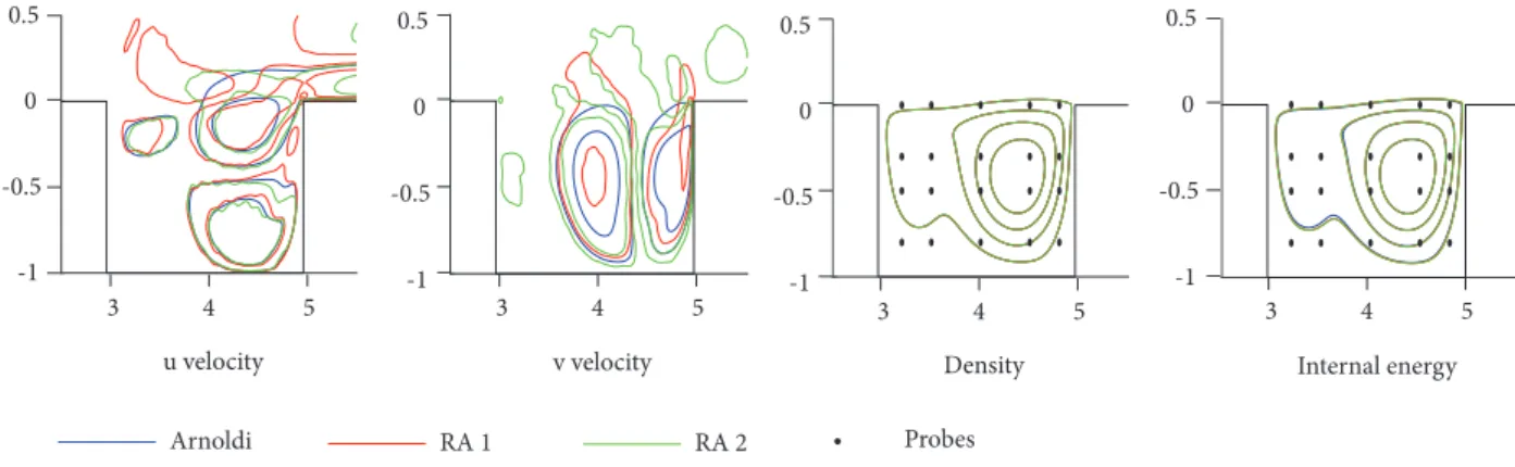
Figure 11 compares the eigenfunctions found by the Arnoldi’s method and by the residual algorithm by ploting the eigenmode’s isocontours for each variable. Two samples of the RA’s eigenfunction are plotted, extracted from different time steps. The probe positions are also shown.
Figure 11. Arnoldi iteration method compared to the residual algorithm.
-8 -6 -4 -2
-1 –0.5
0
0 σ
r
-0.2 –0.1 0
σ
r
σi σi
2 4 6 8
-2 -1.5
-1 -0.5
0 0.5
1 1.5
2 = 1e-2
= 1e-3 = 1e-5 = 1e-7
u velocity -1
-0.5 0
3 4 5 3 4 5 3 4 5 3 4 5
0.5
v velocity -1
-0.5 0 0.5
Density -1
-0.5 0 0.5
Internal energy -1
-0.5 0 0.5
J. Aerosp. Technol. Manag., São José dos Campos, v10, e3718, 2018
The eigenfunction matches for the density and the internal energy, which are the variables the best probes use. For both velocities, the RA has not converged to a single eigenfunction as both samples yielded distinct results, especially just outside of the cavity. MODES RETRIEVED
Figures 12 and 13 show some of the modes retrieved. Mesh 2 was used in this run. Figure 12 shows isocontours of each variable in modes 1 and 2. They are both stationary and their eigenvalues are σ1 = –0.01781 and σ2 = –0.03767, meaning they are stable.
Figure 12. Modes one and two retrieved by the algorithm.
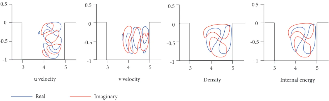
Figure 13 shows mode 4, which is not stationary, therefore has a complex eigenfunction. The isocontours are divided in real and imaginary parts. Its eigenvalue is σ4 = –0.06130 + 0.29274 i.
Figure 13. Mode four retrieved by the algorithm, separated in real and imaginary components.
COMPUTATIONAL COST
For the code performance analysis, a sample case was created. Its mesh has a total of 380 nodes in the stream-wise direction, 170 nodes in the wall-normal direction and 10 nodes in the span-wise direction, including both the physical domain and the buffer zones.
A server running the Ubuntu 14.04 operating system was used. It features 4 Intel® Xeon® E7-4820 v3 processors, each with
10 cores at 1.90 GHz. A total of 128 GB of DDR3 RAM is available.
The code was run for 1000 time steps. About 60 MB of RAM were used for the simulation. Table 3 brings the results for different types of parallel execution.
u velocity -1
-0.5 0
3 4 5 3 4 5 3 4 5 3 4 5
0.5
v velocity -1
-0.5 0 0.5
Density -1
-0.5 0 0.5
Internal energy -1
-0.5 0 0.5
Mode 1 Mode 2
u velocity -1
-0.5 0
3 4 5 3 4 5 3 4 5 3 4 5
0.5
v velocity -1
-0.5 0 0.5
Density -1
-0.5 0 0.5
Internal energy -1
-0.5 0 0.5
J. Aerosp. Technol. Manag., São José dos Campos, v10, e3718, 2018 Mathias MS; Medeiros M
xx/xx 12/13
Table 4. DNS runtime for different parallelization strategies.
Domain slices OpenMP
workers Total threads Runtime (s)
Time per node
per step (s) Speed up
Parallel Efficiency
1 1 1 288.9 4.47 × 10⁻⁶ -
-2 1 2 144.9 2.24 × 10⁻⁶ 99% 99%
1 4 4 122.4 1.89 × 10⁻⁶ 136% 59%
2 4 8 67.5 1.05 × 10⁻⁶ 328% 53%
These runtimes represent a single call to the DNS. Two calls are performed in parallel at each Arnoldi iteration. Computational time spent in the other routines is negligible close to the DNS time. Therefore, the total code runtime can be estimated by multiplying the times presented in this table by the number of Arnoldi iterations.
For example, if this mesh was to be run for 500 iterations, using 16 cores (8 for each DNS instance) the total runtime would be 3375 seconds plus the time spent in the other routines, totaling about 1 hour.
DISCUSSION AND NEXT STEPS
In this work, a tool was developed to analyze the stability of compressible flows over cartesian geometries. It can extract the least stable modes of a flow with relative ease, taking no longer than a few hours in a modern computer for the cases shown here. If the Mach number is increased, this process should be considerably faster, as the DNS can use longer time steps without compromising the numerical stability.
This algorithm is structured in a way that the DNS could be easily replaced with only minor changes to the instability analysis code, meaning that this tool can be adapted for other types of flows, including a three-dimensional analysis or other types of geometries.
An important characteristic of this DNS that is required by the method is a high numerical precision. It is, the ability of resolving many decimal digits without being affected by rounding errors. This is needed due to the large difference in magnitude between the base flow and the disturbances used. A difference of up to seven orders of magnitude between the mean flow velocity and the disturbance RMS was tested and yielded good results.
One intended use for this code is to check if the boundary layer’s stability is affected by small cavities, with a depth about the same size as its displacement thickness.
AUTHOR’S CONTRIBUTION
Conceptualization, Mathias MS and Medeiros M; Methodology, Mathias MS and Medeiros M; Validation, Mathias MS and Medeiros M; Investigation, Mathias MS; Writing – Original Draft, Mathias MS; Writing – Review and Editing, Mathias MS and Medeiros M; Visualization, Mathias MS; Supervision, Medeiros M.
REFERENCES
Åkervik E, Brandt L, Henningson DS, Hœpffner J, Marxen O, Schlatter P (2006) Steady solutions of the Navier-Stokes equations by selective frequency damping. Physics of Fluids 18(6). doi: 10.1063/1.2211705
J. Aerosp. Technol. Manag., São José dos Campos, v10, e3718, 2018 Brès GA, Colonius T (2008) Three-dimensional instabilities in compressible flow over open cavities. Journal of Fluid Mechanics 599:309-339. doi: 10.1017/S0022112007009925
Chiba S (1998) Global stability analysis of incompressible viscous flow. J Japan Soc Comput Fluid Dyn 7(1):20-48.
Colonius T (2001) An overview of simulation, modeling, and active control of flow/acoustic resonance in open cavities. Presented at: 39th Aerospace Sciences Meeting and Exhibit; Reno, USA. doi: 10.2514/6.2001-76
Colonius T, Basu AJ, Rowley CW (1999) Computation of sound generation and flow/acoustic instabilities in the flow past an open cavity. Presented at: 3rd ASME/JSME Joint Fluids Engineering Conference. Proceedings of the Joint Fluids Engineering Conference; San Francisco, USA.
Eriksson LE, Rizzi A (1985) Computer-aided analysis of the convergence to steady state of discrete approximations to the euler equations. Journal of Computational Physics 57(1):90-128. doi: 10.1016/0021-9991(85)90054-3
Gaitonde DV, Visbal MR (1998) High-order schemes for Navier-Stokes equations: algorithm and implementation into FDL3DI. (ADA364301). DTIC Technical Report.
Gómez F, Le Clainche Le, Paredes P, Hermanns M, Theofilis V (2012) Four decades of studying global linear instability: progress and challenges. AIAA Journal 50(12):2731-2743. doi: 10.2514/1.J051527
Gómez Carrasco F, Blackburn H, Rudman M, Sharma A, McKeon B (2015) Manipulating flow structures in turbulent pipe flow. Presented at: 9th International Symposium on Turbulence and Shear Flow Phenomena. Proceedings of the TSFP-9; Melbourne, Australia.
Lele SK (1992) Compact finite difference schemes with spectral-like resolution. Journal of Computational Physics 103(1):16-42. doi: 10.1016/0021-9991(92)90324-R
Li N, Laizet S (2010) 2DECOMP & FFT – a highly scalable 2D decomposition library and FFT interface. Presented at: Cray User Group 2010 Conference; Edinburg, Scotland.
Martínez GAG (2016) Towards natural transition in compressible boundary layers (PhD Thesis). São Carlos: Universidade de São Paulo.
Martínez A, Medeiros MF (2016) Direct numerical simulation of a wavepacket in a boundary layer at Mach 0.9. Presented at: 46th AIAA Fluid Dynamics Conference; Reston, USA. doi: 10.2514/6.2016-3195
Tezuka A, Suzuki K (2006) Three-dimensional global linear stability analysis of flow around a spheroid. AIAA Journal 44(8):1697-1708. doi: 10.2514/1.16632
Theofilis V (2000) On steady-state flow solutions and their nonparallel global linear instability. Advances in Turbulence 8:35-38.
Theofilis V (2003) Advances in global linear instability analysis of nonparallel and three-dimensional flows. Progress in Aerospace Sciences 39(4):249-315. doi: 10.1016/S0376-0421(02)00030-1
Theofilis V (2011) Global linear instability. Annual Review of Fluid Mechanics 43(1):319-352. doi: 10.1146/annurev-fluid-122109-160705