www.hydrol-earth-syst-sci.net/15/3689/2011/ doi:10.5194/hess-15-3689-2011
© Author(s) 2011. CC Attribution 3.0 License.
Earth System
Sciences
Hydro-physical processes at the plunge point: an analysis using
satellite and in situ data
A. T. Assireu1,2, E. Alcˆantara1, E. M. L. M. Novo1, F. Roland3, F. S. Pacheco3, J. L. Stech1, and J. A. Lorenzzetti1 1Remote Sensing Division, National Institute for Space Research, C.P. 515, S˜ao Jos´e dos Campos, SP 12001-970, Brazil 2Natural Resources Institute. Federal University of Itajub´a, UNIFEI, Itajub´a, Brazil
3Aquatic Ecology Laboratory, Biological Science Institute, Federal University of Juiz de Fora, MG, Brazil Received: 14 December 2010 – Published in Hydrol. Earth Syst. Sci. Discuss.: 26 January 2011
Revised: 9 November 2011 – Accepted: 24 November 2011 – Published: 9 December 2011
Abstract. The plunge point is the main mixing point be-tween river and epilimnetic reservoir water. Plunge point monitoring is essential for understanding the behavior of density currents and their implications for reservoir. The use of satellite imagery products from different sensors (Land-sat TM band 6 thermal signatures and visible channels) for the characterization of the river-reservoir transition zone is presented in this study. It is demonstrated the feasibility of using Landsat TM band imagery to discern the subsurface river plumes and the plunge point. The spatial variability of the plunge point evident in the hydrologic data illustrates the advantages of synoptic satellite measurements over in situ point measurements alone to detect the river-reservoir tran-sition zone. During the dry season, when the river-reservoir water temperature differences vanish and the river circulation is characterized by interflow-overflow, the river water inserts into the upper layers of the reservoir, affecting water quality. The results indicate a good agreement between hydrologic and satellite data and that the joint use of thermal and visi-ble channel data for the operational monitoring of a plunge point is feasible. The deduced information about the density current from this study could potentially be assimilated into numerical models and hence be of significant interest for en-vironmental and climatological research.
1 Introduction
According to the report published by the International Com-mittee of Large Dams (ICOLD; www.icold-cigb.net) in 2000, over 40 000 large dams exist in the world, with a to-tal storage capacity of 7000 billion m3. An average of 0.5 to
Correspondence to:A. T. Assireu ([email protected])
1 % of their capacity is lost each year due to sedimentation. Changes due dams can include increased depth, changes in temperature, the possible development of density stratifica-tion, the retention of nitrate and phosphate, the growth of plankton and algae, contaminant trends in sediment, changes in the aquatic ecosystem from lotic to lentic, and the release of carbon-based greenhouse gases (Baxter, 1997; Poff and Hart, 2002; Ramos et al., 2006).
Because the density of the river water reaching a voir usually differs from the density of the water at the reser-voir surface, inflows enter and move through the reserreser-voir as density currents (Ford, 1990). Temperature, total dissolved solids, and suspended solids can cause density differences. Depending on the density difference between the inflows and ambient waters, the density currents in a reservoir can flow into the downstream area as overflow, underflow, or interflow types (Martin and McCutheon, 1999).
Thus, after the inflow plunges the river, it can follow the thalweg as an underflow. It is frequently assumed that once an inflow has plunged into a reservoir and formed an under-flow or interunder-flow, its constituent load is isolated from the sur-face waters. Although this situation has been shown to be true in many cases, recent studies (Chen et al., 2006) have indicated that mixing can entrain inflow constituents into sur-face waters.
It is not uncommon for environmental fluids to be sub-jected simultaneously to the destabilizing effects of a veloc-ity shear stress (induced by underflow) and to the stabilizing effects of density stratification. The outcome of such com-petition is often the Kelvin-Helmholtz (KH) instability (e.g. DeSilva et al., 1996; Thorpe and Jiang, 1998; ¨Ozg¨okmen and Chassignet, 2002; Umlauf and Lemmin, 2005). The result-ing entrainment has been extensively studied elsewhere (e.g. Chung and Gu, 1988; Gu and Chung, 2003).
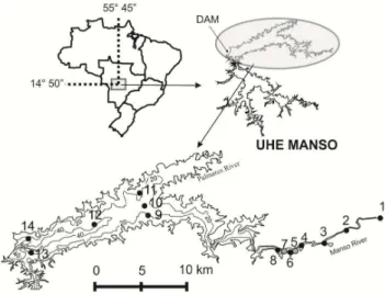
Fig. 1. Study area and bathymetry of Manso reservoir with con-tours at 20-m intervals. The grey circles (temperature, fluores-cence and photosynthetically available radiation [PAR]) and filled circles (temperature, conductivity, dissolved oxygen, fluorescence and photosynthetically available radiation PAR) mark the sampling and transect stations. Position 13 also indicates the location of the limnolo-meteorological station (SIMA), MAN-13. The locations of the thermistor chain and drifter deployments are indicated by posi-tion 8.
water characteristics. Density currents may transport unde-sirable materials, such as suspended solids, organic chem-icals, or nutrients from the watershed, to reservoirs down-stream (Chen et al., 2006) or may cause sedimentation (An-nandale, 1987; De Cesare et al., 2001). Thus, appropriate reservoir operation to avoid sedimentation or water quality deterioration requires knowledge of density current behavior. Some studies regarding density currents have been car-ried out in the Feitsui Reservoir (Chen et al., 2006), Lake Ogawara (Dallimore et al., 2001) and the Katsyrasawa Reser-voir (Chikita, 1989) in Japan, Lake Geneva in Switzerland (Lambert and Giovanoli, 1988), Lake Onachota and Fayet-teville Green Lake in the United States (Ford, 1990), and the Alpine Luzzone Reservoir in Switzerland (De Cesare et al., 2001). To our knowledge, there have been no studies re-porting the use of remote sensing to study the plunge point location in reservoirs.
The available literature uses visible channel data to look at changes in the clarity and color of the water (Chipman et al., 2004) associated with changes in sediment input (Mertes et al., 1993) or the amount of chlorophyll (Novo et al., 2006) due to algal blooms (Duan et al., 2009) and uses thermal infrared data to look at changes in the surface temperature (Alcˆantara et al., 2010) associated with upwelling (Schladow et al., 2004; Steissberg et al., 2005) or changes in circulation (Ikeda and Emery, 1984).
Some authors (e.g. Anderson et al., 1995) deployed a hand-held thermal radiometer to obtain indirect
measure-ments of the water surface temperatures to study the influx of cold water in reservoirs. However, this kind of data is lim-ited in time and space. The knowledge of the physical, chem-ical, and biological mechanisms controlling water quality is limited by a lack of observations at the spatial density and temporal frequency needed to infer the controlling processes. The ability when using satellite images to combine synoptic information with temporal recovering makes remote sensing a very useful tool to study plunge point locations.
The plunge point location indicates where the riverine zone stops and the lake zone begins. If the riverine zone extends a significant distance into the reservoir, the reservoir is dominated by advective forces and cannot be considered to be vertically one-dimensional (Arneborg et al., 2004). Be-cause the processes occurring in a reservoir are dependent on the river behavior along the reservoir, which is strongly de-termined by the contrast between incoming river water and reservoir water, remote sensing can be used to study some important aspects of reservoir functioning. It is important because, depending on the location, in situ measurements of temperature, such as those provided by the use of thermistor chains, might not capture the plunge point spatial variability and, consequently, might not be useful to determine if the inflow will behave as an under, inter or overflow.
A number of models have been proposed to predict plunge depth (Dallimore et al., 2004). These models are generally valid only for channels with a constant slope and width. The failure to accurately predict the plunge depth will result in an inaccurate representation of the initial underflow layer thick-ness and therefore cause a distortion of the underflow dynam-ics beyond the plunge point (Dallimore et al., 2004).
Based on this, the purpose of this paper is to jointly ap-ply thermal and visible satellite instruments, in situ data and satellite-tracked drifters to monitor the density current be-tween a water body and the inflowing water (at the plunge point location).
2 Methods
2.1 Field site and measurements
The Manso Reservoir (14◦50′S; 55◦45′W), located in a Brazilian savanna biome, has a dendritic shape with 427 km2 of flooded area and a maximum depth of 60 m (Fig. 1).
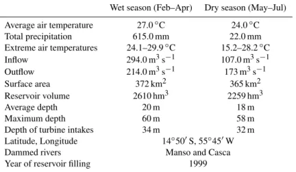
Table 1.Mean general characteristics of Manso Reservoir.
Wet season (Feb–Apr) Dry season (May–Jul)
Average air temperature 27.0◦C 24.0◦C
Total precipitation 615.0 mm 22.0 mm
Extreme air temperatures 24.1–29.9◦C 15.2–28.2◦C
Inflow 294.0 m3s−1 107.0 m3s−1
Outflow 214.0 m3s−1 173 m3s−1
Surface area 372 km2 365 km2
Reservoir volume 2610 hm3 2259 hm3
Average depth 20 m 18 m
Maximum depth 60 m 58 m
Depth of turbine intakes 34 m 32 m
Latitude, Longitude 14◦50′S, 55◦45′W
Dammed rivers Manso and Casca
Year of reservoir filling 1999
measured for each sample station according to Eaton and Franson (2005).
2.2 Environmental time series
The temporal variability of the environmental parameters used here was measured using data collected with an an-chored buoy system, the Integrated System for Environmen-tal Monitoring (SIMA). This system is a set of hardware and software designed for data acquisition and the real-time monitoring of hydrological systems (Stech et al., 2006), with fixed data storage systems, sensors (air temperature, wind direction and intensity, pressure, incoming and reflected ra-diation and a thermistor chain), a solar panel, a battery and a transmission antenna.
The data were collected in preprogrammed time intervals and were transmitted by satellite in quasi-real time for any user within a range of 2500 km from the acquisition point. The selection of the environmental parameters measured us-ing the SIMA (moored near the dam, indicated by Station-13 in Fig. 1) took into account aspects including the relevance as an environmental index (i.e. the variables that respond con-sistently to alterations in the functioning of an aquatic sys-tem), the importance of the greenhouse gas-emission process in aquatic systems, and the technical suitability for data ac-quisition and transmission from automatic platforms (Stech et al., 2006).
2.3 Environmental profiles
Vertical profiles were measured during the wet season (Fig. 1) as follows: (1) eleven stations were oriented in the longitudinal direction from the river (stations 1 to 8) toward the dam (stations 10, 12 and 13), following the thalweg, and (2) three stations were oriented in the transverse direction. This design allowed for the construction of one
longitudi-nal transect composed of 11 profiles and two transverse tran-sects, one near the dam (stations 13 and 14) and the other 20 km from the dam (stations 9, 10 and 11) (Fig. 1).
The stations were spaced 3 km apart in the reservoir and 0.5 km apart in the rireservoir transition zone. The ver-tical profiles of pressure, water temperature (with a resolu-tion of 0.01◦C and 5 % accuracy), dissolved oxygen con-centration (resolution: 0.01 mg l−1and accuracy: 2 %), and conductivity (resolution: 1.0 µS cm−1 and accuracy: 0.5 %) were made with a multi-parameter probe (Yellow Springs In-str., model 6600) and a submersible fluorimeter (Satlantic) with a resolution of 0.05 µg l−1and range of 0–200 µg l−1.
A total of 56 contained Hobo temperature loggers were de-ployed in five thermistor chains at 1-m intervals from depths 0 to 4 m and at 3-m intervals from depths 4 to 20 m. The sampling period of the thermistor was 15 min.
2.4 Circulation measurements
The water circulation measurements in the river-reservoir transition zone were carried out using drifters. These drifters were built following the design developed by Sybrandy and Niiler (1991) and consisted of a GPS data logger installed in a spherical fiberglass float and connected to a drogue to re-duce the wind-slip effect. The drifters were drogued at 6 m because the focus in the present experiment was on the inflow velocity. This depth was selected based on the temperature profiles obtained with the multi-parameter probe.
series were filtered using a low-pass filter with a cutoff period of 15 min.
2.5 Computing water surface temperature from Landsat-5-TM data
Generally, the grey level in images from the Thematic Map-per (TM) sensor of the Landsat satellites is given as a digital number (DN) ranging from 0 to 255 (8 bits). Thus, the com-putation of the brightness temperature from TM6 (thermal band: 10.5–12.5 µm) data includes the estimation of radi-ance from its DN value and the conversion of the radiradi-ance into brightness temperature.
For this purpose, we utilized the equation developed by the National Aeronautics and Space Administration (NASA),
T= K2 lnK1
Lλ+1
, whereT is the effective at-satellite tempera-ture in kelvin,K2 andK1 is the calibration constant 2 and 1 in kelvin (W m−2sr−1µm−1), respectively (Chander et al., 2009). The water vapor content and atmospheric temperature in each layer were approximated using local meteorological observation data (Qin et al., 2001), measured at the Weather Forecast and Climatic Studies Center (CPTEC) of the Brazil-ian National Institute for Space Research (INPE).
2.6 Wedderburn and Lake numbers
The Wedderburn number,W= c2h (u2
∗L), was calculated
follow-ing the method of Imberger and Patterson (1990). W is the ratio of the maximum baroclinic pressure force (before the upwind surfacing of the thermocline) and the surface wind force. The relevant internal gravity-wave speed was calcu-lated asc=pg′h. The dynamic balance defined byW was extended with the vertically integrated Lake number (LN,
Imberger and Patterson, 1990; Stevens and Imberger, 1996). This quantity is defined asLN=
gSt
1−zTH
ρu∗A1.5
1−zgH, where gis gravity,ρis the density of water,zT is the height of the
cen-ter of the metalimnion,zgis the height of the center of
vol-ume of the lake,Ais the lake area,His the depth of the lake,
u∗is the friction velocity in water andSt (g cm−1cm−2)is
an estimate of the stability of the reservoir calculated asSt=
Rzm
0 (z−zg)A(z)ρ(z)dz(Hutchinson, 1957). As Stevens and Imberger (1996) have shown,St can be considered as an
in-tegral equivalent toW.
2.7 The entrainment velocity, the depth of the plunge point, and the Kelvin-Helmholtz instability
Some authors (Britter and Linden, 1980; Monaghan et al., 1999) have found from theory and laboratory experiments that the head of density currents travels at a constant speed,
UF, which is proportional to a third power of the buoyancy
flux per unit width, defined asBF =g′Q, whereg′ (the
re-duced gravity) is equal tog1ρp/ρo(where1ρpis the density difference across the pycnocline,ρois mean density, andg
is gravity) andQ=hrUr is the volume flux per unit width,
withhr andUr being the average thickness and speed,
re-spectively, of the current at the input location. Studying grav-ity and densgrav-ity currents, ¨Ozg¨okmen and Chassignet (2002) showed that numerical simulations compare well with labo-ratory measurements and that labolabo-ratory results are valid on geophysical scales.
The depth (m) of the plunge point was estimated with the following equation (Ford, 1990):
h=1.6 Q 2
gL2|1ρρ|
!1/3
(1)
wherehis the hydraulic plunge point depth (m),1ρ is the difference between the densities of the inflow and reservoir water (kg m−3), and L is the width of the convergence zone (m).
The density function, developed by Gill (1982) and Ford (1990), is presented in the following equations:
ρ=ρTw+1ρs (2)
ρTw =999.8452594+6.793952×10⁻²Tw
−9.095290×10⁻³Tw2+1.001685×10⁻⁴Tw3
−1.120083×10⁻⁶Tw4+6.536332×10⁻⁹Tw5 (3)
1ρs=Css
1− 1
sg
×10−3=0.00062Css (4) whereρTw is the density of water and is a function of wa-ter temperature (Tw),1ρsis the density increment owing to the concentration of suspended solids (Css), and “sg” is the specific gravity of suspended solids, assumed as reported by Chen et al. (2006).
The entrainment coefficient, E, and the normal depth of the underflow along the centerline, hc, were calculated as reported by Chen et al. (2006) using the following equations:
E=1
2CkC 3/2
d F
2 (5)
hc= 6E
5 × +hr (6)
wherex is the distance downstream from the plunge point andF is the Froude number at a plunge point, defined as follows:
F2= U 2 r
g|1ρρ|h (7)
by a factor of two, the speed and height change by 20–25 %. A model of a frictionally balanced gravity current (Stige-brandt, 1987) was used to compare the speed (u) estimated using the modelUr=
s cdg
1ρ ρ h
1/2
with that measured us-ing the drifters.
3 Results and discussion
3.1 Meteorological conditions and thermal structure
The temporal patterns of rainfall, wind and air temperature (Fig. 2a) and short- and long-wave radiation (Fig. 2b) show that the daily precipitation can exceed 80 mm during the wet season in the studied region. As detailed below, the result-ing increases in the inflow have a strong effect on the ther-mal structure of the reservoir during the wet season. In the dry season the long-term decreasing trend in the short-wave radiation and increase in the wind speed are easily seen. Southwesterly winds were predominant in dry season (win-ter), when speeds reached up to 8.0 m s−1, with an average 3.5±1.8 m s−1. The predominant southwesterly direction coincides with the direction of main Manso Reservoir fetch (Fig. 1).
At the end of April and July, seven cold-front events reached Manso Reservoir (arrows in Fig. 2a). Further de-tails about the action of cold fronts in Manso Reservoir were reported by Lorenzzetti et al. (2005). Each peak of the wind speed was associated with a steep decrease of the air tem-perature during the cold-front passage. The air temtem-peratures declined by approximately 6◦C during these events, and the daily average wind speed reached 6 m s−1.
Because the latent and sensible flux terms are almost lin-early dependent on the wind and the short-wave drops dur-ing the cold-front passage, the net surface radiation becomes negative, and the reservoir loses (latent) heat to the atmo-sphere (data not shown). Thus, the deepening of the surface mixed layer due to the stirring from the wind stress will be enhanced by downward convective mixing during dry sea-sons, as observed in Lake Victoria, East Africa, by MacIntyre et al. (2002).
The thermal stratification in Manso Reservoir is moderate and is spread over a thick metalimnion during the first half of the analyzed period (2 February–30 April) (Figs. 3 and 4). The metalimnion extends from 7–25 m, with tempera-tures ranging from 28–30◦C. During this period, the wind speed averaged 2.3±0.5 m s−1, without any predominant di-rection. The stability of the water column, given in Hz by
N=(gρ−1∂ρ/∂z)1/2 (g, acceleration due to gravity; ρ is water density), was solely temperature-dependent (salinity
∼0.02 ‰ calculated from conductivity) and showed values within 5–18 cph [N(cph) = (3,600/2π )×N(Hz)], reflecting a moderate stratification (Fig. 1b) Values around 20 cph corre-spond to strongly stratified oceanic waters (MacIntyre et al., 2002).
Fig. 2.Daily means of air temperature, wind speed and precipitation (upper panel) and the daily means of solar short-wave radiation and long-wave fluxes (lower panel) from February to July 2007.
During the stratified period of the wet season, the thick metalimnion and moderate stratification could make Manso Reservoir susceptible to partial upwelling (W >
2 or LN<10), i.e. metalimnetic water reaching the sur-face. However, an analysis based on the Wedderburn and Lake Number (Fig. 4) indicates that the wind-driven up-welling/downwelling was unimportant during the wet sea-son. Some enhanced mixing events are visible during 16– 19 February, 18–21 March, and 6–9 May, when water of 28◦C was transported to the surface.
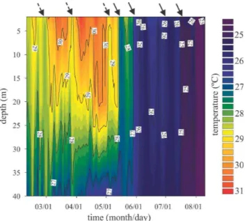
In the next section, we show evidence regarding the con-tribution of the river to enhancing the mixing process, indi-cated by arrows in Fig. 3. The reservoir thermal structure (Fig. 4) suggests that in the wet season, the river stays at the hypolimnion level and contributes to the thermal stability of the water column. This situation persists during the wet sea-son. In the dry season, the river circulation is characterized by interflow-overflow, as discussed below.
3.2 River effects on the thermal structure and Kelvin-Helmholtz instability
In situ measurements during the wet season showed a high contrast between the suspended solid concentrations in the reservoir (4.2 mg l−1)and river water (15.0 mg l−1). This contrast can be easily observed in the satellite images (Fig. 5a). This contrast is also observed in the surface water temperatures (Fig. 5b).
Fig. 3. Temperature contours (◦C) from the thermistor-chain data measured near the dam (MAN-13). Arrows indicates mixing process.
uppermost portion of the water column (such as chlorophyll, inorganic particles and dissolved organic matter), whereas the thermal radiation detects skin temperatures.
The turbidity currents can be observed in Fig. 5a to travel underwater until they reach a depth at which the sensor can no longer detect them. Thus, the true plunge point posi-tion is given by the thermal image. In the dry season, the plunging point location in the visible-spectrum satellite im-age (Fig. 5c) is consistent with that of the thermal imim-age (Fig. 5d).
As noted by Ford (1990), these water density differ-ences are mainly caused by differdiffer-ences in temperature and dissolved- or suspended-solid loads throughout the river-reservoir transition. According to Akiyama and Stefan (1984), these physicochemical patterns cause density differ-ences between the reservoir and river waters, which are re-sponsible for the plunging inflows.
Manso Reservoir experiences large seasonal and short time runoff variations. As a result, the inflow variations present an intermittent pattern, with large inflows during the summer and autumn months (Fig. 6a). This fact suggests that the inflow controls the residence time for Manso Reservoir, as verified by Rueda et al. (2006) for the Sau Reservoir. The estimated power spectra at the thermocline displacement and the buoyancy flux due to inflow show similar variabilities, with frequencies between 0.3 and 0.6 cpd (Fig. 6b).
If the peaks in the range of 0.3–0.6 cpd were indicative of an interchange between thermocline oscillation and buoy-ancy flux, the peaks would be coherent but out of phase be-cause the signal of inflow must be propagated 23 km down-stream to the thermistor chain. If the signal had a
propa-23
Fig. 4. Temporal evolution of the thermal structure (upper panel) and the Wedderburn and Lake numbers (lower panel) at Station 13.
gation speeduof approximately 0.1 m s−1(as estimated us-ing a model and confirmed usus-ing the drifter data) over a dis-tance of 23 km, the propagation time would be approximately 2.5 days. The coherence spectra (Fig. 6c) indicate that mo-tions in the range of 0.3–0.6 cpd are coherent and are 120◦ out of phase (Fig. 6d). This result suggests that the inflow is an important mechanism driving the thermocline displace-ment.
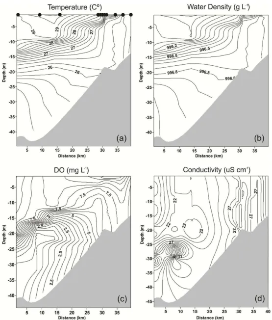
The river water progressively sinks down to the level of the thermocline and contributes to the thermal stability of the water column during the wet season (Fig. 7). After the inflow plunges, it can follow the thalweg as an underflow partially enhanced by downstream turbine and spillway outflows (out-flow at Manso∼15 m).
The river water had a similar temperature, conductivity, and pH as the hypolimnion (Figs. 7, 8) at the dam area (39 km downstream of the river), indicating that the river followed the thalweg as an underflow. In this case, during the wet sea-son, the following fluid behavior is expected: a denser fluid enters a domain and flows under a lighter fluid, waves de-velop along the interface (due to shear velocity), and these waves grow in the downstream direction, develop into bil-lows and eventually roll up. This behavior is indicative of the Kelvin-Helmholtz instability, in which waves made up of fluid from the current (river) entrap the ambient fluids (Thorpe and Jiang, 1998; Corcos and Sherman, 2005).
The usual condition for the onset of Kelvin-Helmholtz instability is that the gradient Richardson number, Ri=
g ρo
∂ρ ∂z
∂U ∂z
−2
, must be lower than a critical value, typically
Ricrit∼=0.25.
Fig. 5.Satellite images (in true-color composition) acquired on 26 March(a)and 16 July(c), showing the seasonal plunge point variation (red circles), and the water surface temperature (b,d) estimated from the thermal band (band 6) of Landsat 5 TM.
24
02/09 03/01 03/21 04/10 04/30 05/20 06/09 06/29 07/19 08/080 100 200 300 400 500 600 700 800 900 1000
Time (day)
inflow (m3s-1) outflow (m3s-1)
(a)
0 0.1 0.2 0.3 0.4 0.5 0.6
0 0.2 0.4 0.6 0.8 1
Frequency (cpd)
C
o
h
e
re
n
c
e
(c)
0 0.1 0.2 0.3 0.4 0.5 0.6
-120 -60 0 60 120 180
Frequency (cpd)
P
h
a
s
e
(
d
e
g
re
e
s
)
(d)
Fig. 6. (a)Inflow and outflow,(b)power spectra of the time evolution of the thermocline displacements and buoyancy flux smoothed by three Hanning passes (the 95 % confidence interval is indicated),(c)coherence (the 5 % level for zero coherence is indicated) and(d)the relative phase for the thermocline and buoyancy flux.
is Richardson-number dependent. Some authors (Kunze et al., 1990; Trowbridge, 1992; Peters et al., 1995; Baringer and Price, 1997) show that theRiestimates are very sensitive
to the length scale over which the vertical gradients are cal-culated. Thus, we apply in our analysis an alternative toRi
Figure 7: Isopleths of the (a) water temperature, (b) density, (c) dissolved oxygen and
Fig. 7.Isopleths of the(a)water temperature,(b)density,(c)dissolved oxygen and(d)conductivity in Manso Reservoir during March (wet season). The dots at top of temperature panel correspond to longitudinal transects.
performed by Cushman-Roisin (2005) and yielded a criterion for the vertical extent of the eventual mixing. If the following inequality holds true, (ρ2−ρ1)gH
ρo(U1−U2)2
<1, then vertical mixing is energetically possible.
To evaluate the typical vertical velocity shear, the cur-rent measured using the drifters in the river-reservoir tran-sition zone was analyzed. The mean difference between the currents at 6 m and 2 m was approximately 6.0 cm s−1 (Fig. 9b). This difference (U1−U2), applied in the above in-equality, indicates that the Kelvin-Helmholtz instability may play a strong role in the thermocline displacement during the wet season. Alongshore components of the drifter velocity (Fig. 9a) show the anisotropy in the mean kinetic energy.
During the dry season, the decrease in the river flow and the decrease in density differences (Fig. 5d) lead to river cir-culation characterized by inter-overflow. As discussed, many cold-front passages occurred during this period. Thus, im-portant energetic mixing processes are driven by winds and by surface cooling during the dry season due to cold-front action, and hence, the closer the river water is to the surface, the higher is the probability that it experiences mixing with the reservoir waters.
Fig. 8.Temperature, conductivity, and pH vertical profiles at Manso Reservoir measured in the river and at the MAN-13 station during the wet season.
27
Fig. 9. (a)Alongshore and crossshore current velocity component and(b)speed at 1.0 and 6.0 m of depth (January).
Available nutrients can be assimilated by phytoplankton and may stimulate plankton blooms. In the downstream direc-tion, where an inter-overflow would hit the dam construcdirec-tion, an accumulation of phytoplankton could occur and may be seen from satellite imagery (Fig. 10). This process affected the water quality: the concentrations of suspended solids at the surface varied from 2.2 to 4.8 mg l−1(dry season – inter-overflow) and dropped to the range between 0 to 1.0 mg l−1 (rainy season – underflow) in the reservoir, while in the river, this concentration was 15 mg l−1 and 10 mg l−1 during the dry season and the rainy season, respectively.
Fig. 10. (a)Satellite imagery in a normal composition (RGB-321) showing the area with a chlorophyll bloom (from the left up to the dashed contour). (b)The same satellite imagery with a land mask and enhanced contrast to better discriminate the phytoplank-ton bloom (16 July 2007).
: Temperature contours from the thermistor-chain data measured at Fig. 11.Temperature contours from the thermistor-chain data mea-sured at the river-reservoir transition zone (January) (Station 06).
Fig. 12.Temperature contours from the thermistor-chain data mea-sured near the dam (January) (Station 08).
a Secchi disk) in Manso Reservoir, when the transparency dropped from 5.5 m to 4.5 m. Through these results, we will pass to discuss the plunging underflow in more detail.
3.3 Analysis of a plunging underflow
The important density current parameters (i.e. propagation speed, thickness, and the point of plunging) can be used to determine a change in water quality at different depths (Alavian et al., 1992). Despite the limited predictive abil-ity of empirical models, due to the complex bathymetry of real reservoirs and continuous rather than layered stratifica-tion (Dallimore et al., 2004), which indicates the need for observations of density currents, we used a simplified one-dimensional model (Eqs. 1–7) to estimate and compare the model predictions with the hydrological data. The thermal structure, shown in Fig. 11, and the average inflow water temperature (26.5◦C) were utilized.
Based on the measured suspended solid concentrations in the river, the inflow suspended solid concentration was 15 mg l−1. The estimated total density of the inflow, in-cluding the density increment due to suspended solids, was 996.53 kg m−3. The reservoir mean water temperature was 28◦C, and the density difference between the inflow and reservoir water was 0.62 kg m−3. The Froude number (Eq. 7) of the flow was estimated to be 0.198, and the estimated depth of the plunge point was 10.5 m, which is close to the observed depth, 12 m (Fig. 10). The entrainment coefficient,
E, was 0.00031.
Applyinghin Eq. (6), the greatest depth (hc) that would have been reached by the density current was estimated to be 14.5 m atx=20 km. This estimated value is very close to that observed from the thermistor chain positioned 20 km
downstream (Fig. 12). The estimated result is thus consistent with the observed data.
4 Conclusions
With the objective of monitoring the plunge-point location in the Manso hydroelectric reservoir, the following conclusions were demonstrated:
– The spatial variability of the plunge point, evident in the hydrologic data, illustrates the advantages of synoptic satellite measurements over in situ point measurements alone to detect the river-reservoir transition zone. – During the wet season, the upward entrainment
engen-dered by the Kelvin-Helmholtz instability was the main mixing mechanism in the reservoir waters.
– During the dry season, when the river and reservoir wa-ter temperatures were nearly homogeneous, the river circulation was characterized by inter-overflow. – The joint use of thermal and visible channel data for
the operational monitoring of the plunge point is feasi-ble. The deduced information about the density current from this study could potentially be assimilated into nu-merical models and hence be of significant interest for environmental and climatological research.
Acknowledgements. This work was supported by the “Carbon Budgets of Hydroelectric Reservoirs of Furnas Centrais El´etricas S. A.” project. The authors are grateful to the Brazilian Council for Scientific and Technological Development (CNPq) for the grants 482488/2007-7. The authors wish to express their gratitude to the reviewers, whose comments and suggestions were very helpful.
Edited by: A. Gelfan
References
Akiyama, J. and Stefan, H. G.: Plunging flow into reservoir: The-ory, J. Hydraul. Eng., 110, 484–499, 1984.
Alavian, V., Jirka, G. H., Denton, R. A., Johnson, M. C., and Stefan, H. G.: Density currents entering lakes and reservoirs, J. Hydraul. Eng., 18, 1464–1489, 1992.
Alcˆantara, E. H., Stech, J. L., Lorenzzetti, J. A., Bonnet, M.-P., Casamitjana, X., Assireu, A. T., and Novo, E. M. L. M.: Remote sensing of water surface temperature and heat flux over a tropical hydroelectric reservoir, Remote Sens. Environ., 114, 2651–2665, 2010.
Anderson, J. M., Duck, R. W., and Mcmanus, J.: Thermal radiome-try: a rapid means of determining surface water temperature vari-ations in lakes and reservoirs, J. Hydrol., 173, 131–144, 1995. Eaton, A. D. and Franson, M. A. H.: American Water Works
Annandale, G. W.: Reservoir sedimentation, Elsevier Science Pub-lishers: Amsterdam, 1987.
Arneborg, L., Erlandsson, B. L., and Stigebrandt, A.: The rate of inflow and mixing during deep-water renewal in a sill fjord, Lim-nol. Oceanogr., 49, 768–777, 2004.
Baringer, M. O. and Price, J. F.: Momentum and energy balance of the Mediterranean outflow, J. Phys. Oceanogr., 27, 1678–1692, 1997.
Baxter, R. M.: Environmental effects of dams and Impoundments, Ann. Rev. Ecol. System., 8, 255–283, 1997.
Britter, R. E. and Linden, P. F.: The motion of the front of a gravity current traveling down an incline, J. Fluid Mech., 99, 531–543, 1980.
Chander, Q., Markham, B. L., and Helder, D. L.: Summary of cur-rent radiometric calibration coefficients for Landsat MSS, TM, ETM+, and EO-1 ALI sensors, Remote Sens. Environ., 113, 893–903, 2009.
Chen, Y. J., Wu, S. C., Lee, B. S., and Hung, C. C.: Behavior of storm-induced suspension interflow in subtropical Feitsui Reser-voir, Taiwan, Limnol. Oceanogr., 51, 1125–1133, 2006. Chikita, K.: A field study on turbidity currents initiated from spring
runoffs, Water Resour. Res., 25, 257–271, 1989.
Chipman, J. W., Lillesand, T. M., Schmaltz, J. E., Leale, J. E., and Nordheim, M. J.: Mapping lake water clarity with Landsat im-ages in Wisconsin, U.S.A., Can. J. Remote Sensing., 30, 1–7, 2004.
Chung, S. and Gu, R.: Two-dimensional simulation of contaminant currents in a stratified reservoir, J. Hydr. Eng., 124, 704–711, 1988.
Corcos, G. M. and Sherman, F. S.: The mixing layer: deterministic models of a turbulent flow, J. Fluid Mech., 139, 29–65, 2005. Cushman-Roisin, B.: Kelvin-Helmholtz Instability as a
Boundary-value Problem, J. Fluid Mech., 5, 507–525, 2005.
Dallimore, C. J., Imberger, J., and Ishikawa, T.: Entrainment and turbulence in saline underflow in Lake Ogawara, J. Hydraul. Eng., 127, 937–947, 2001.
Dallimore, C. J., Imberger, J., and Hodges, B. R.: Modeling a Plunging Underflow, J. Hydraul. Eng., 130, 1068–1076, 2004. De Cesare, C., Schleiss, A., and Hermann, F.: Impact of turbidity
currents on reservoir sedimentation, J. Hydraul. Eng., 127, 6–16, 2001.
DeSilva, I., Fernando, H. J. S., Eaton, F., and Hebert, D.: Evolu-tion of Kelvin-Helmholtz billows in nature and laboratory, Earth Planet. Sci. Lett., 143, 217–231, 1996.
Duan, H., Ma, R., Xu, X., Kong, F., Zhang, S., Kong, W., Hao, J., and Shang, L.: Two-decade reconstruction of algal blooms in china’s lake taihu, Environ. Sci. Technol., 43, 3522–3528, 2009. Ford, D. E.: Reservoir Transport Processes, in: Reservoir Limnol-ogy: Ecological Perspectives, edited by: Thornton, K. W., Kim-mel, B. L., Payne, F. E., Wiley-Interscience: New York, pp. 15– 41, 1990.
Gill, A. E.: Appendix 3: Properties of seawater, in: Atmosphere-ocean dynamics, edited by: Gill, A. E., Academic press: New York, 1982.
Gu, R. and Chung, S.: A two-dimensional model for simulating the transport and fate of toxic chemicals in a stratified reservoir, J. Environm. Quality., 32, 620–632, 2003.
Hutchinson, G. E.: A treatise on limnology, geography, physics and chemistry, John Wiley, 1015 p., 1957.
Ikeda, M. and Emery, W. J.: A continental-shelf upwelling event off Vancouver Island as revealed by satellite infrared imagery, J. Mar. Res., 42, 303–317, 1984.
Imberger, J. and Patterson, J. C.: Physical limnology, Adv. Appl. Mech., 27, 303–475, 1990.
Kunze, E., Williams, A. J., and Briscoe, M. G.: Observations of shear and vertical stability from a neutrally buoyant float, J. Geo-phys. Res., 95, 18127–18142, 1990.
Lambert, A. and Giovanoli, F.: Records of riverborne turbidity cur-rents and indications of slope failures in the Rhone delta of Lake Geneva, Limnol. Oceanogr., 33, 458–468, 1988.
Lorenzzetti, J. A., Stech, J. L., Assireu, A. T., Novo, E. M. L. M., and Lima, I. B. T.: SIMA: a near real time buoy acquisition and telemetry system as a support for limnological studies, in: Global warming and hydroelectric reservoirs, edited by: Santos, M. A. and Rosa, L. P., COPPE: Rio de Janeiro. pp. 71–79, 2005. MacIntyre, S., Romero, J. R., and Kling, G. W.: Spatial-temporal
variability in surface layer deepening and lateral advection in an embayment of Lake Victoria, East Africa, Limnol. Oceanogr., 47, 656–671, 2002.
Martin, J. L. and McCutheon, S. C.: Hydrodynamics and transport for water quality modeling, Lewis, 1999.
Mertes, L. A. K., Smith, M. O., and Adams, J. B.: Estimating sus-pended sediment concentrations in surface waters of the Amazon River wetlands from Landsat images, Remote Sens. Environ., 43, 281–301, 1993.
Monaghan, J. J., Cas, R. A. F., Kos, A. M., and Halworth, M.: Grav-ity currents descending a ramp in a stratified tank, J. Fluid Mech., 379, 39–70, 1999.
Novo, E. M. L. M., Barbosa, C. C., Freitas, R. M., Shimabukuro, Y. E., Melack, J. M., and Pereira Filho, W.: Seasonal changes in chlorophyll distributions in Amazon floodplain lakes derived from MODIS images, Limnology, 7, 153–161, 2006.
¨
Ozg¨okmen, T. M. and Chassignet, E. P.: Dynamics of
two-dimensional turbulent bottom gravity currents, J. Phys. Oceanogr., 32, 1460–1478, 2002.
Peters, H., Gregg, M. C., and Sanford, T. B.: Detail and scaling of turbulent overturns in the Pacific equatorial undercurrent, J. Geophys. Res., 100, 18349–18368, 1995.
Poff, N. L. and Hart, D. D.: How dams vary and why it matters for the Emerging Science of Dam Removal, Bioscience, 52, 659– 668, 2002.
Qin, Z., Karnieli, A., and Berliner, P.: A mono-window algorithm for retrieving land surface temperature from Landsat TM data and its application to the Israel-Egypt border region, Int. J. Re-mote Sensing., 22, 3719–3746, 2001.
Ramos, R. M., Lima, I. B. T., Rosa, R. R., Mazzi, E. A., Carvalho, J. C., Rasera, M. F. F. L., Ometto, J. P. H. B., Assireu, A. T., and Stech, J. L.: Extreme event dynamics in methane ebullition fluxes from tropical reservoirs, Geophys. Res. Lett., 33, L21404, doi:10.1029/2006GL027943, 2006.
Rueda, F., Moreno-Ostos, E., and Armengol, J.: The residence time of river water in reservoirs, Ecolog. Modelling., 191, 260–274, 2006.
Schladow, S. G., Palmarsson, S. O., Steissberg, T. E., Hook, S. J., and Prata, F. J.: An extraordinary upwelling event in a deep ther-mally stratified lake, Geophys. Res. Lett., 31, 1–4, 2004. Stech, J. L., Lima, I. B. T., Novo, E. M. L. M., Silva, C. M., Assireu,
Rosa, R. R.: Telemetric monitoring system for meteorological and limnological data acquisition, Verh. Internat. Verein. Lim-nol., 29, 1747–1750, 2006.
Stevens, C. and Imberger, J.: The initial response of a stratified lake to a surface shear stress, J. Fuid Mech., 312, 39–66, 1996. Steissberg, T. E., Hook, S. J., and Schladow, S. G.:
Character-izing partial upwelling and surface circulation at Lake Tahoe, California-Nevada, USA with thermal infrared images, Rem. Sens. Environ., 99, 2–15, 2005.
Stigebrandt, A.: A model for the vertical circulation of the Baltic deep water, J. Phys. Oceanogr., 17, 1772–1785, 1987.
Sybrandy, A. L. and Niiler, P. P.: WOCE/TOGA Lagrangian drifter-construction manual, University of California: California, 1991. Thorpe, S. A. and Jiang, R.: Estimating internal waves and diapy-cnal mixing from conventional mooring data in a lake, Limnol. Oceanogr., 43, 936–945, 1998.
Trowbridge, J. H.: A simple description of the deepening and struc-ture of a stably stratified flow driven by a surface stress, J. Geo-phys. Res., 97, 15529–15543, 1992.